2.1 Parallel-lane corridor model and basic rules

Using the existing procedures for RNAV Q-routes as a basis for flow corridor design^(10,23), the flow corridor analysed here is represented by a tube of parallel high-altitude routes structure which is designed to be 80 nm long and 16 nm wide with the route centrelines 8 nm apart and located at FL350, as shown in Fig. 1. Based on the prototype spacing and passing capability for speed-independent tracks^{(Reference Wing, Smith and Ballin5)}, pilots of the aircraft are responsible for self-separation aided by automation through Airborne Collision Avoidance System (ACAS), ADS-B and PBN capabilities including the provision of conflict resolution advisories⁽²⁴⁾. Aircraft travel in the same direction from the entrance to exit. In the case of a faster aircraft behind a slower aircraft, pilots can adjust the velocity of the former and separation with the leading one, switch lanes for overtaking, or in extreme cases exit the corridor along paths that are at a divergence angle of 30° before the exit. Additional details of the movement rules of each aircraft in the corridor are designed as follows:

1. 1. All aircraft initially enter the corridor with random types, velocities and separations with their leading ones, and the initial velocities are set as their target velocities in the corridor.

2. 2. Each aircraft is in level flight along the middle line of each corridor and self-separates with the aircraft in front according to a self-separation model by adjusting its acceleration and velocity.

3. 3. Whenever the velocity of an aircraft is higher than the average velocity of the leading one by a velocity threshold, and the separation is smaller than a specified distance threshold, it attempts to switch the lane.

4. 4. Whenever an aircraft gets within the minimum separation standard of the aircraft in front (loss of the minimum separation), it switches its lane or breaks out.

5. 5. Any aircraft whose separation with its leading one is larger than a specified distance threshold value, it flies towards the target velocity.

6. 6. The first aircraft in each lane always flies towards its target velocity.

Figure 1 Structure of corridor.

2.2 Aircraft dynamic model

An aircraft in the flow corridor is modelled using the Point Mass Model (PMM) developed by Glover and Lygeros^{(Reference Glover and Lygeros25)}. The aircraft motion is captured by a control system with six states (horizontal position, the altitude of the aircraft, the true airspeed, the flight path angle and the heading) and three inputs (the engine thrust, the bank angle and the angle-of-attack) as Tables 1 and 2.

Table 1 State variables

Table 2 Control variables

The equations for level flight in the flow corridor now become

(1) $$\left\{ \matrix{ \dot{\rm x}{\equals}v\cos {\rm \rpsi }\cos {\rm \rgamma } \hfill \cr \dot{\rm v}{\equals}{1 \over m}(T\cos { \ralpha }{\minus}D{\minus}mg\sin {\rm \rgamma }) \hfill \cr \dot{\rpsi }{\equals}{1 \over {m}{\rm v}}(L{\plus}T\sin {\rm \ralpha })\sin \rphi \hfill \cr \dot{\rgamma }{\equals}{1 \over {m}{\rm v}}[(L{\plus}T\sin {\rm \ralpha })\cos \rphi {\minus}mg\cos {\rm \rgamma }] \hfill \cr} \right.$$

where m is the mass of the aircraft and g is the gravitational acceleration. L and D denote, respectively, the lift and drag forces, which are functions of the state and the angle-of-attack as follows:

(2) $$\left\{ \matrix{ L{\equals}{{C_{L} S\rrho v^{2} } \over 2} \hfill \cr D{\equals}{{C_{D} S\rrho v^{2} } \over 2} \hfill \cr} \right.$$

where S is the surface area of the wings, ρ is the air density and C _D , C _L are aerodynamic lift and drag coefficients whose values generally depend on the phase of the fight. During the cruising phase, all commercial airliners are usually operating near trimmed flight conditions ( $\gamma {\equals}\dot{\gamma }{\equals}0$ and α≈0)^{(Reference Palm26)}, and then the lift is represented by

(3) $$\eqalignno{ \dot{\rgamma }{\equals} & {1 \over {m}{\rm v}}[(L{\plus}T\sin {\rm \ralpha })\cos \rphi {\minus}mg\cos {\rm \rgamma }]{\equals}0 \cr \hskip-11pt \Rightarrow L{\equals}mg{{\cos {\rm \rgamma }} \over {\cos \rphi }}{\minus}T\sin {\rm \ralpha }{\equals}{{mg} \over {\cos \rphi }} $$

Assume that the coefficient of lift C _L is set so that the lift exactly balances the weight of the aircraft. Combining the previous relationships, C _L can be calculated by

(4) $$\eqalignno{ L{\equals} & {{mg} \over {\cos \rphi }}{\equals}{{C_{L} S\rrho {\rm v}^{2} } \over 2} \cr \hskip-12pt\Rightarrow C_{L} {\equals}{{2mg} \over {S\rrho {\rm v}^{2} \cos \rphi }} $$

The drag coefficient during the cruising phase is computed as follows:

(5) $$C_{D} {\equals}C_{{{\rm D0}}} {\plus}C_{{{\rm D2}}} C_{L}^{2} $$

where C _D0 and C _D2 are two constants.

3.1 Self-separation performance states definition

In order to describe self-separation performance of aircraft in the flow corridor, five discrete states are defined: Self-separation State (SS), Target Velocity Flying State (TVFS), Lane Changing State (LCS), Breakout State (BS) and Locking State (LS).

(a) Self-separation State (SS)

SS is a state in which an aircraft attempts to adjust the velocity and acceleration according to the longitudinal separation and velocity difference with its leading aircraft. An aircraft is in this state if its separation with the leading one is less than the distance threshold (that means, the leading aircraft is not too far in front) but larger than the minimum separation (the distance-based separation minima for aircraft self-separating in the flow corridor for safety operation consideration). Combining the equations of the time derivatives of the along-track positions and velocities in Equation (1), we obtain

(6) $$\left\{ \matrix{ \dot{\rm x}{\equals}{\rm v}\cos {\rm \rpsi }\cos {\rm \rgamma } \hfill \cr \dot{{\rm v}}{\equals}{1 \over m}(T\cos {\rm \ralpha }{\minus}D{\minus}mg\sin {\rm \rgamma }) \hfill \cr} \right.$$

Because all the aircraft are assumed straight (ψ=0 or small) and level flight ( $\gamma {\equals}\dot{\gamma }{\equals}0$ , α=0) in the corridor, substitute the drag in Equation (2) into the above equations and get

(7) $$\left\{ \matrix{ \dot{\rm x}\,\approx\,{\rm v} \hfill \cr \dot{{\rm v}}{\equals}{T \over m}{\minus}{{C_{D} S\rrho } \over {2m}}{\rm v}^{2} \hfill \cr} \right.$$

This is equivalent to a second-order equation:

(8) $$\ddot{x}{\equals}{T \over m}{\minus}{{C_{D} S\rrho } \over {2m}}{\rm v}^{2} $$

Using a proportional plus derivative control for aircraft thrust (T)^{(Reference Palm26)} yields

(9) $$T{\equals}k(x_{{{\rm ref}}} {\minus}x){\plus}c({\rm v}_{{{\rm ref}}} {\minus}{\rm v}){\plus}T_{{{\rm ref}}}$$

where T _ref is the thrust of the aircraft to balance the drag (Equation (2)), k and c are two tuning parameters used for keeping the target aircraft within the appropriate separation and velocity limits. x _ref is the target position along the track which equals to the along-track position of the leading aircraft minus the Target Separation (the proposed longitudinal separation to keep with the leading aircraft for safety) between the two consecutive aircraft. v _ref is the target velocity equal to that of the leading aircraft during the self-separating period. This leads to the second-order system as

(10) $$\eqalignno{ \ddot{x}{\equals} & {{k(x_{{{\rm ref}}} {\minus}x){\plus}c({\rm v}_{{{\rm ref}}} {\minus}{\rm v}){\plus}{{C_{D} S\rrho } \over 2}{\rm v}^{2} } \over m}{\minus}{{C_{D} S\rrho } \over {2m}}{\rm v}^{2} \cr \hskip-12pt \Rightarrow {m}\ddot{x}{\plus}c\dot{\rm x}{\plus}kx{\equals}kx_{{{\rm ref}}} {\plus}c{\rm v}_{{{\rm ref}}}$$

Translating Equation (3) into the matrix notation, yields

$$\eqalignno{ & {\bf X}{\equals}\left[ {\matrix{ {x_{1} } \cr \vdots \cr {x_{n} } \cr } } \right],\quad {\bf X}_{{{\bf ref}}} {\equals}\left[ {\matrix{ {x_{{1,\; {\rm ref}}} } \cr \vdots \cr {x_{{n,\; {\rm ref}}} } \cr } } \right],\quad {\bf V}_{{{\bf ref}}} {\equals}\left[ {\matrix{ {v_{{1,\; {\rm ref}}} } \cr \vdots \cr {v_{{n,\; {\rm ref}}} } \cr } } \right], \quad {\bf M}{\equals}\left[ {\matrix{ {m_{1} } & {} & {} \cr {} & \ddots & {} \cr {} & {} & {m_{n} } \cr } } \right],\quad \cr &{\bf C}{\equals}\left[ {\matrix{ {c_{1} } & {} & {} \cr {} & \ddots & {} \cr {} & {} & {c_{n} } \cr } } \right],\quad {\bf K}{\equals}\left[ {\matrix{ {k_{1} } & {} & {} \cr {} & \ddots & {} \cr {} & {} & {k_{n} } \cr } } \right] $$

Thus, the self-separation system in the corridor can be denoted in matrix notation is given by

(11) $${\rm M}\ddot {\rm X}{\plus}{\rm C}\dot{\rm X}{\plus}{\rm KX}{\equals}{\rm CV}}_{{{\rm ref}}} {\rm {\plus}KX}_{{{\rm ref}}} $$

To calculate the value of matrix C and K, given that an un-damped natural frequency matrix is

$${\rm \Omega }{\equals}\left[ {\matrix{ {\romega _{1} } & {} & {} \cr {} & \ddots & {} \cr {} & {} & {\romega _{n} } \cr } } \right]{\equals}\left[ {\matrix{ {\sqrt {{{k_{1} } \over {m_{1} }}} } & {} & {} \cr {} & \ddots & {} \cr {} & {} & {\sqrt {{{k_{n} } \over {m_{n} }}} } \cr } } \right]$$

Given also that the damping ratio of an aircraft i is

(12) $${\rm \rzeta }_{i} {\equals}{{c_{i} } \over {2\sqrt {m_{i} k_{i} } }}$$

From the above, a time constant of τ _i can be achieved as follows, and leading to the determination of c _i

(13) $${\rm \rtau }_{i} {\equals}{1 \over {{\rm \rxi }_{i} {\rm \romega }_{i} }}{\equals}{{2\sqrt {m_{i} k_{i} } } \over {c_{i} }}\sqrt {{{m_{i} } \over {k_{i} }}} {\equals}{{2m_{i} } \over {c_{i} }}\Rightarrow c_{i} {\equals}{{2m_{i} } \over {\rtau _{i} }}$$

A damping ratio of ζ _i can be achieved as follows, leading to the determination of k _i

(14) $${\rm \rzeta }_{i} {\equals}{{c_{i} } \over {2\sqrt {m_{i} k_{i} } }}\Rightarrow k {\equals}{{c_{i}^{2} } \over {4m_{i} {\rm \rzeta }_{i} ^{2} }}$$

Using τ ₁ and ζ _i as input, and with the values of C and K, the accelerations of all the aircraft for the self-separation can be calculated as Equation (5):

(15) $${\ddot{\rm X}{\rm {\equals}M}^{{{\minus}{\rm 1}}} {\rm (K(X}_{{{\rm ref}}} {\minus}{\rm X){\plus}C(V}_{{{\rm ref}}} {\minus}{\dot{\rm X}))}}$$

(b) Target Velocity Flying State (TVFS)

TVFS is a state in which an aircraft attempts to fly at its preferred target velocity without regard to the position or velocity of the aircraft in front of it. An aircraft is in this state if either (a) it is the first aircraft in the lane or (b) its leading aircraft is sufficiently far ahead (the separation is larger than the distance threshold) so that it does not currently need to adjust its velocity to maintain separation. Without considering the position of leading aircraft (k=0), the second-order system for TVFS can be derived from Equation (10) as follows:

(16) $$m\ddot{x}{\plus}c\dot{\rm x}{\plus}kx{\equals}kx_{{{\rm ref}}} {\plus}c{\rm v}_{{{\rm ref}}} \Rightarrow m\ddot{x}{\plus}c\dot{\rm x}{\equals}c{\rm v}_{{{\rm ref}}}$$

where v _ref is the target velocity equal to its initial velocity when the aircraft enters the flow corridor. The longitudinal acceleration of the aircraft can be updated as

(17) $$\ddot{x}{\equals}{{c({\rm v}_{{{\rm ref}}} {\minus}\dot{\rm x})} \over m}$$

(c) Lane Changing State (LCS)

LCS is a state in which an aircraft switches its lane to another with constant velocity for overtaking or avoiding loss of the minimum separation. An aircraft switches lanes under the following two situations: (a) it is traveling at a higher velocity necessitating an overtaking manoeuvre or (b) to avoid loss of the minimum separation. In the LCS state, the target aircraft flies a 30º (θ) path to another lane with a constant velocity as shown in Fig. 2. The constant velocity is set as the final speed before changing to the LCS state. The projection position (x _projection) can be calculated based on the aircraft along-track position (x), the two-lane centre distance (W) and the turning angle (θ) as Equation (18). The traveling distance (D _switch) for switching the lane is shown in Equation (19), and the across track position(y) can be derived based on trigonometric function.

Figure 2 Lane changing state.

(18) $$x_{{{projection}}} {\equals}x{\minus}W\,{\rm tan}{{\rm \rtheta } \over 2}$$

(19) $$D_{{{switch}}} {\equals}{W \over {\sin {\rm \rtheta }}}\\\,$$

(d) Locking state (LS)

LS is a combined state used for safety and efficiency consideration. This state always works with the SS and TVFS states to prevent simultaneous lane changes or breakouts. When an aircraft is in the LCS, the trailing aircraft in the original corridor will be in the LS state (be locked) for one-time step in order to avoid two consecutive aircraft changing to the LCS or the BS at the same time. Furthermore, the leading and trailing aircraft in the new corridor are locked until the corridor switch procedure is finished for safety. This is to prevent two aircraft from ‘crossing’ in the middle while changing lanes. Figure 3 illustrates a scenario of LSs. As stated earlier, the consideration of safety is a largely deterministic process based on known failure modes and the incorporation of barriers, in this case through the LS. The effects of unknown failures and different sources of uncertainty including human factors or errors will be considered in the future to improve the models in this paper.

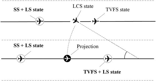
Figure 3 Locking states.

(e) Breakout state (BS)

An aircraft breaks out of the corridor if it cannot switch lane to avoid loss of the minimum separation. BS is a terminal state in which a target aircraft follows a route to breakout to the side of a corridor as shown in Fig. 4. The breakout aircraft keeps its velocity and adjusts its horizontal position until it is out of the corridor region. The trailing aircraft in the original corridor is locked for one-time step to avoid two consecutive aircraft changing to the BS or the LCS at the same time.

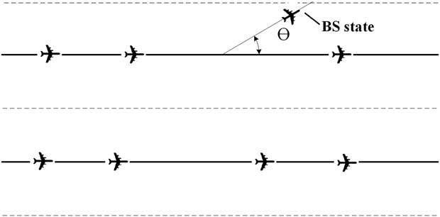
Figure 4 Breakout state.

3.2 The main simulation algorithm

The main algorithm for self-separation is as follows: each aircraft is initialised with the SS, and the model checks the separations and velocity differences between the aircraft and their leading ones for state transition. If the current separation with the leading aircraft is larger than the distance threshold, the preceding aircraft transfers to the TVFS.

If the velocity difference is equal to or greater than the velocity difference threshold, and also the current separation is less than the lane-switch threshold, then the lane-switch requirement is checked. This represents a scenario where the two aircraft are close to each other and the trailing aircraft is traveling at a higher velocity necessitating an overtaking manoeuvre.

If the lane-switch requirement is satisfied, the trailing aircraft transfers to the LCS and flies with a constant velocity to the other lane. The aircraft in the other lane will self-separate with the lane-switching aircraft by adjusting the separation with the estimated merge point. Both the new leading and trailing aircraft in the other lane are transferred to the LS until the lane-switch manoeuvre is finished. If the lane switch requirement cannot be satisfied, the aircraft transfers to the SS state (current separation is larger than the minimum separation) or BS state (current separation is smaller than the minimum separation).

If the velocity difference is smaller than the velocity difference threshold, and the current separation is larger than the minimum separation, the trailing aircraft changes to the SS state. Otherwise, the trailing aircraft checks the lane-switch requirement for lane switch. This represents a case where the trailing aircraft is traveling at a velocity that is either slower or only slightly faster than the leading aircraft but the current separation cannot satisfy the minimum separation requirement, some potential conflicts might happen.

If the lane-switch requirement is satisfied, the trailing aircraft transfers to the LCS and some relative flights transfer to the LS; otherwise, it transfers to the BS. Figure 5 shows the main algorithm flowchart for aircraft states transitions.

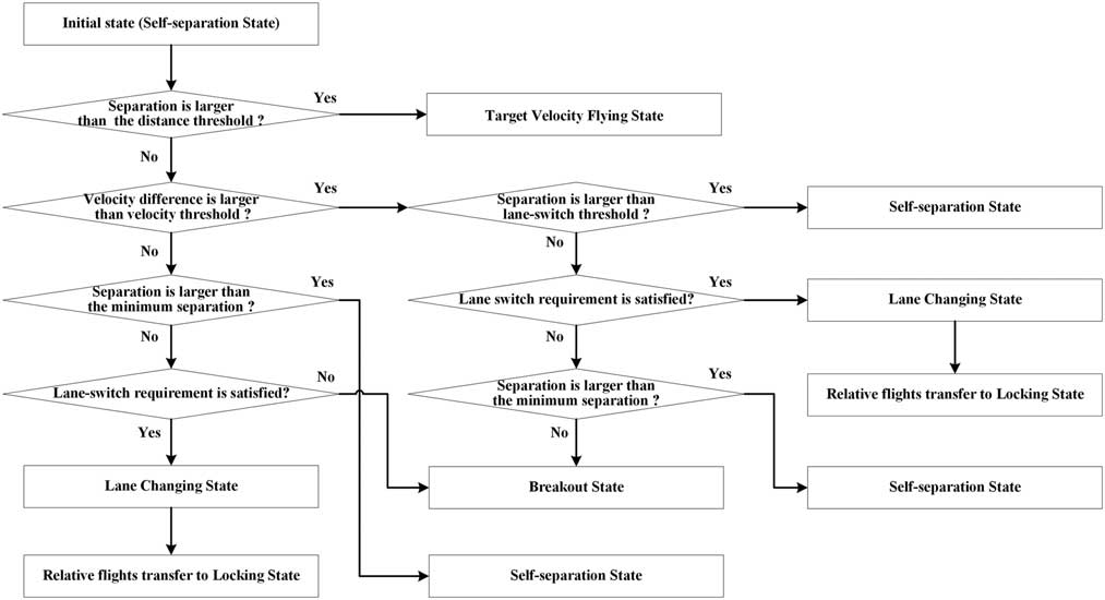
Figure 5 State transition flowchart.

The lane-switch requirement is defined as (a) the potential lane-switch aircraft should be in either the SS or TVFS state without being locked; (b) the potential lane-switch aircraft should make a projection of the target flight onto another lane (30° path) to find its new leading and trailing aircraft in that lane, and both of the distances between the potential lane-switch aircraft and the new leading and trailing aircraft must be larger than the lane-switch threshold; (c) the trailing aircraft in the new lane should also be in the SS or the TVFS without being locked.

3.3 Key parameters

3.3.1 Simulation inputs

The inputs of the simulation can be divided into four types: corridor geometry parameters, aircraft performance parameters, simulation control parameters and self-separation parameters. Among these, the self-separation parameters are the key inputs which have significant impacts on the capacity and conflicts of the corridor. Table 3 presents and describes these inputs, including the initial separation, minimum separation, buffer separation, target separation, velocity difference threshold, distance threshold and lane-switch threshold.

Table 3 Self-separation inputs

3.3.2 Capacity and conflict metrics

Table 4 illustrates the capacity and conflicts for the flow corridor in this paper. Capacity is measured by the flow corridor throughput which is defined as the number of aircraft that can fly through the flow corridor per hour (not including the breakout aircraft).

Table 4 Capacity and safety metrics

Conflicts are measured by the conflict rate, lane-switch rate and breakout rate in the corridor which belongs to the strategic intent-based conflict detection and resolution safety level^{(Reference Zhang, Shortle and Sherry22)}. The lane-switch rate is the proportion of aircraft that switch from one lane to another for overtaking or avoiding the loss of the minimum separation which is considered as resolvable conflict rate in the corridor. The breakout rate is the proportion of aircraft that must leave the corridor to avoid a subsequent loss of minimum separation which is considered as un-resolvable conflict rate in the corridor. The conflict rate is defined as the total conflict rate for both the resolvable and un-resolvable conflict rate in the flow corridor which is obtained by the sum of lane-switch rate and breakout rate.

4.1 Experiments design and parameters setting

The simulation program is written in the C++ language and visually verified by Google Earth. The simulated aircraft trajectories were converted to KML format, which can be read by Google Earth and displayed in an animated fashion, as in Fig. 6.

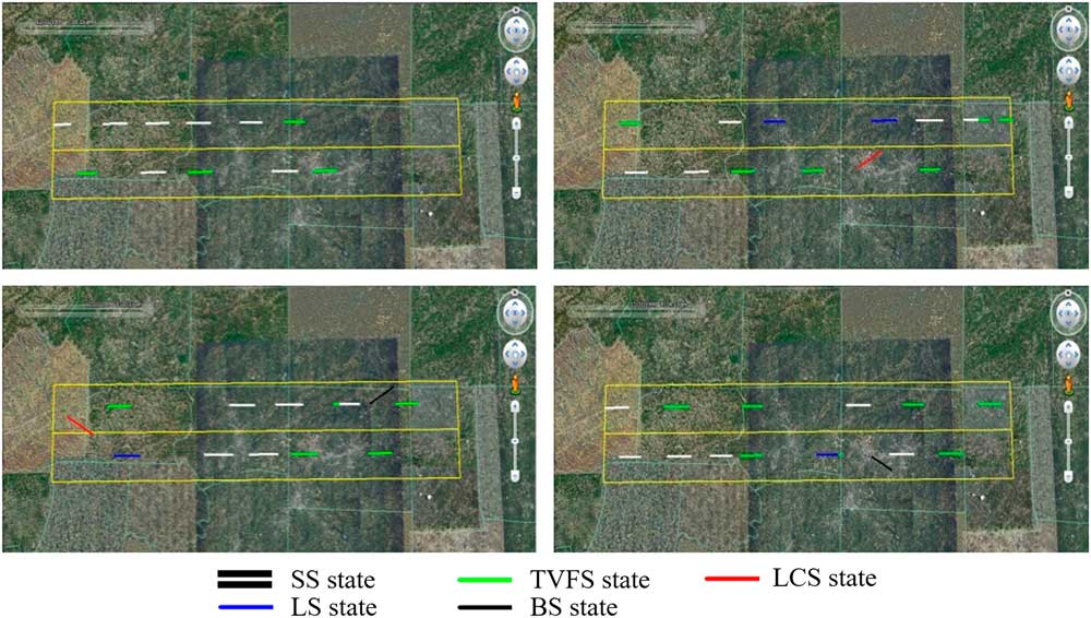
Figure 6 (Colour online) Visual verification by Google Earth.

Both practical data and Pseudo-random numbers are used in the simulation. The simulation program has a total of 98 scalar parameters.

The aircraft performance parameters used in this research come from the User Manual for the Base of Aircraft Data (BADA)⁽²⁷⁾ published by EUROCONTROL. Eight typical aircraft types, A320, A332, A345, A380, B737, B742, B743, and B764, are selected for simulations. Table 5 shows some aircraft performance data which are taken from the BADA library, including the reference mass (m _ref), the maximum operational Mach number (M_MO), standard cruise Mach number above Mach transition altitude (M_CR) and maximum longitudinal acceleration for civil flights (a _{I, max}). Each flight enters the flow corridor with random aircraft type and follows the standard cruise Mach number, M_CR, the velocity and acceleration of each flight cannot be larger than the M_MO and a _{I, max} at any time.

Table 5 Aircraft performance parameters

For the self-separation parameters’ values, to make sure that the variables are independent of each other, two more parameters, which are the extra switch-buffer and extra threshold-buffer, are introduced in the experiments. Then, the target separation is defined as the sum of the minimum separation and separation buffer, the lane-switch threshold is defined as the sum of the target separation and extra switch buffer, and the distance threshold is defined as the sum of lane-switch threshold and extra threshold buffer. Thus, the initial separation, minimum separation, separation buffer, extra switch buffer, extra threshold buffer and velocity threshold are regarded as independent variables, and the initial values of some key simulation parameters are shown in Table 6.

Table 6 Initial values of some key simulation parameters

4.2 Sensitivity analysis

In the experiment, in order to take into account the traffic flow pattern variations caused by different levels of severe weather, and make sure that each aircraft enters the corridor following the current ICAO aircraft separation regulations⁽²⁸⁾, the initial separation value is set as 5 nm (the longitudinal separation minima) plus a random buffer that follows an exponential distribution with the mean ranges from 1 to 10 nm. Subsequent analysis addressed the sensitivity of the other independent variables including the separation buffer, minimum separation, extra switch-buffer, extra threshold buffer and velocity difference threshold. The throughput, conflict rate, breakout rate and lane-switch rate are four metrics used for performance evaluation.

4.2.1 Initial separation and separation buffer

Figure 7 reflects the changes in the four metrics with the increase of separation buffer from 0.5 nm to 10 nm in 0.5 nm steps, and other parameters are set as initial values in Table 6. In general, with the increase of initial separation, both the throughputs and conflict rates are reducing consistently, which are in conformity with the ‘larger initial separation makes for safer flying’ intuition. However, with the increase of separation buffer, associated curves show different change trends.

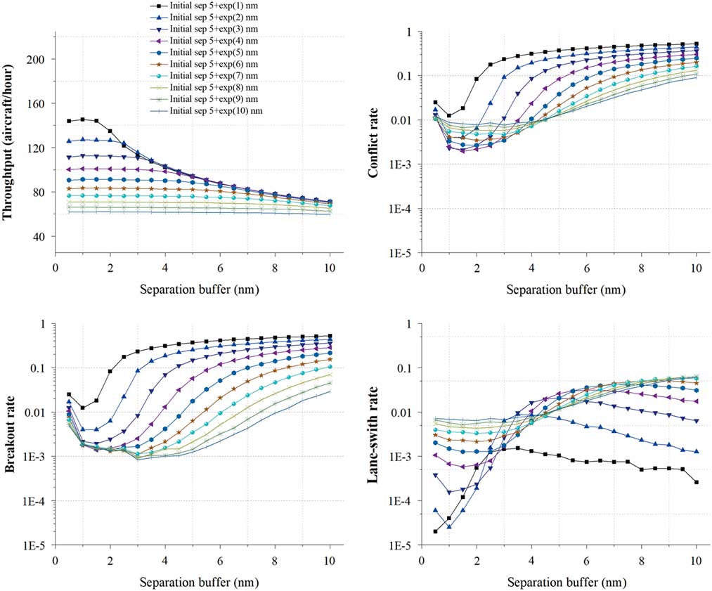
Figure 7 (Colour online) Initial separation and separation buffer.

For the throughput, there is an obvious hump-shape configuration in the relation between the throughput and the separation buffer, but the hump shape shrinks and disappears gradually with the increase of initial separation. When the initial separation equals 5+exp (1) nm, the throughput increases from 143.81 to 145.31 aircraft/hour at first, then decreases quickly to only 71.12 aircraft/hour. As the initial separation increases to 5+exp (10) nm, no hump exists anymore and the throughput curve shows only a slight and steady decrease from 61.58 to 59.54 aircraft per hour.

For the conflict rate, associated curves show a similar ‘decrease–increase’ trend with the increase of separation buffer, also these ‘decrease and increase’ gradients are getting smaller with the increase of separation buffer. When the initial separation equals to 5+exp (1) nm, the conflict rate drops drastically from 0.0248 to 0.0124 first, and then rises sharply to over 0.5223. As the initial separation increases to 5+exp (10) nm, after an initial quick drop, the conflict rate decreases gradually to 0.0076, and then increases mildly to 0.0906. In addition, as the main components of the conflict rate, the breakout rate curves also show a similar ‘decrease–increase’ trend with the conflict rate curves while the lane-switch rate curves show some fluctuation variation.

These trends indicate that there is an interesting correlation between the initial separation and separation buffer. And after detailed analysis, we find the reason is that the increase of the separation buffer will lead to higher target separation, and the extreme values of the minimum throughput and conflict rate are both obtained when the initial separation is close to the target separation. Another point worth noting is that the lane-switch rate not strictly followed this rule, which means that larger separation buffer also leads to larger lane-switch threshold, thus decreases the chance of lane-switch for the potential conflicts.

4.2.2 Initial separation and minimum separation

Figure 8 reflects the changes in the four indicators with the increase of minimum separation from 2 nm to 11.5 nm with 0.5 nm per step, and other parameters are set as initial values in Table 6. In general, with the increase of the initial separation, the throughput is reducing consistently while the conflict rate curves show an ‘increase and decrease’ change which breaks the intuition of ‘larger initial separation makes for safer flying’. And with the increase of separation buffer, both the throughput and the conflict rate show a slight downward trend at the beginning, and then the throughput curves show an obvious downward trend while the conflict rate curves show a quick increase trend.

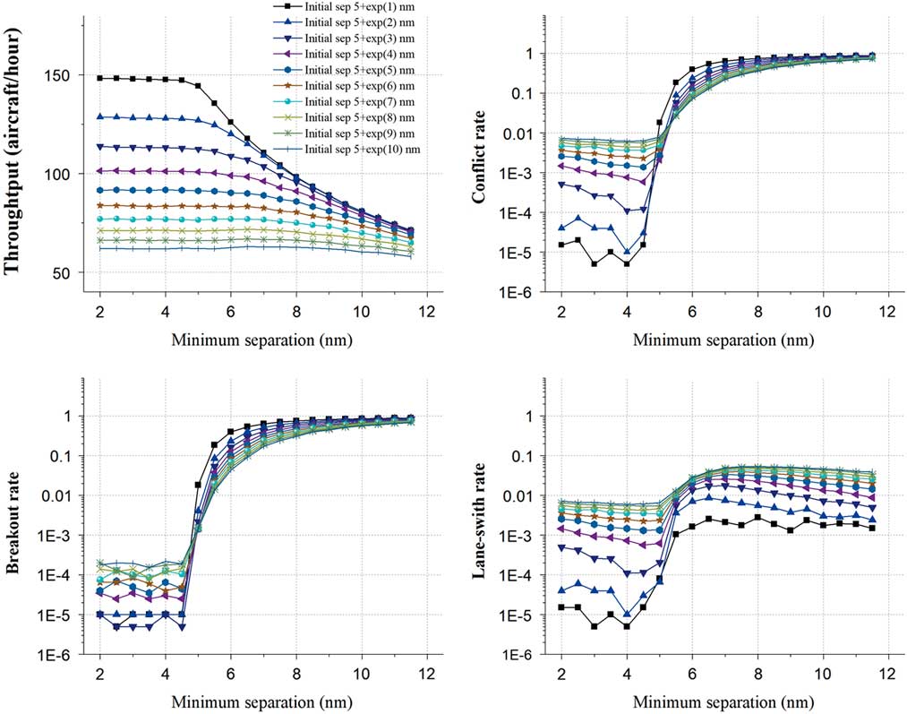
Figure 8 (Colour online) Initial separation and minimum separation.

For the throughput, when the initial separation equals 5+exp (1) nm, the throughput keeps slight decrease from 148.17 to 147.11 aircraft/hour, after that it decreases quickly to 71.18 aircraft/hour. As the initial separation increases to 5+exp (10) nm, instead of the ‘steady and decrease’ trend, the throughput stays stable at about 61.54 aircraft/hour.

For the conflict rate, when the initial separation equals 5+exp (1) nm, the conflict rate decreases slightly from 0.000015 to 0.000005 first, and then increases to 0.8858 quickly. As the initial separation increases to 5+exp (10) nm, the conflict rate drops slightly from 0.0073 to 0.0062 first, and then increases to 0.7187 quickly. As the principal components, both the breakout rate and the lane-switch rate show a similar ‘decrease and increase’ trend as the conflict rate. However, a noticeable trend is that the all the lane-switch rate curves increase monotonically with the increase of the minimum separation while there is some crossing point for both the conflict rate and breakout rate curves.

These trends may indicate that since the target separation will rise with the increase of the minimum separation, aircraft have to reduce the speeds to enlarge the separations with their leading ones, which will slow down the traffic flows and reduce the throughputs. Also, both the throughput and the conflict rate show tremendous changes after some threshold value in the figure which may be caused by the enlarger of the difference between the initial separation and the target separation. In addition, with the increases of the target separation, the space and chance for lane-switching are reduced gradually which leads to the decrease of the lane-switch rate again after some threshold value.

4.2.3 Initial separation and extra switch buffer

Figure 9 reflects the changes in the four indicators with the increase in the extra switch buffer from 0 nm to 4 nm in 0.2 nm steps, and other parameters are set as initial values in Table 6. In general, with the increase of initial separation, the throughput is consistently reducing while the conflict rate curves show a ‘decrease and increase’ trend. However, with the increase of extra switch buffer, both the throughput and the conflict rate curves seem to fluctuate within a narrow range.

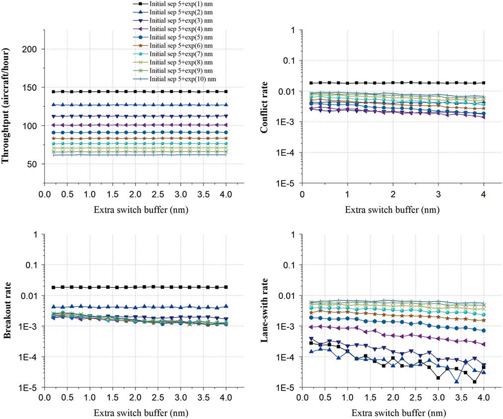
Figure 9 (Colour online) Initial separation and Extra switch-buffer.

For the throughput, when the initial separation equals 5+exp (1) nm, the throughput achieves the maximum mean value and stays around 144.18 aircraft/hour. As the initial separation increases to 5+exp (10) nm, the throughput stays at around 61.79 aircraft/hour.

For the conflict rate, when the initial separation equals 5+exp (1) nm, the conflict rate achieves the maximum mean value of 0.0184, and then decreases gradually to the minimum value at around 0.0021 as the initial separation increases to 5+exp (3) nm. After that, the conflict rate rises again to 0.008 gradually with the increase of the initial separation to 5+exp (10) nm. This interesting result is that the effect of the combination of the breakout rate and lane-switch rate. Both of these two metrics show a similar ‘decrease and increase’ change but with different extreme values. The breakout rate obtains the maximum mean value of 0.0183 when the initial separation equals 5+exp (1) and the minimum mean value of 0.0015 when the initial separation equals 5+exp (5). The lane-switch rate obtains the maximum mean value of 0.0063 when the initial separation equals 5+exp (10) and the minimum mean value of 0.00008 when the initial separation equals 5+exp (2).

These trends may indicate that different extra switch buffer may has little effect on the four metrics, but with the initial separation, there are still some joint impacts on the conflict rates, breakout rates and lane-switch rates.

4.2.4 Initial separation and extra threshold buffer

Figure 10 reflects the changes in the four indicators with the increase in the extra threshold buffer from 5 nm to 14.5 nm in 0.5 nm steps, and other parameters are set as initial values in Table 6. In general, with the increase of initial separation, the throughput is consistently reducing while the conflict rate curves show a ‘decrease and increase’ trend. Also, with the increase of extra threshold buffer, the throughput seems to keep steady while the conflict rate curves show some downward trends.

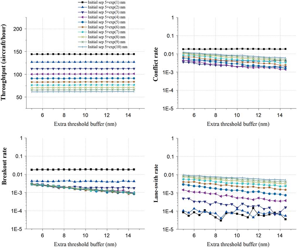
Figure 10 (Colour online) Initial separation and extra threshold buffer.

For the throughput, when the initial separation equals 5+exp (1) nm, the throughput achieves the maximum mean value of 144.18 aircraft/hour. As the initial separation increases to 5+exp (10) nm, the throughput stays at around 61.74 aircraft/hour.

For the conflict rate, when the initial separation equals 5+exp (1) nm, the conflict rate achieves the maximum mean value and stays around 0.0184, and when the initial separation equals 5+exp (3) nm, the conflict rate achieves the minimum mean value of 0.0023. After that, the mean value of conflict rate rises again to 0.0086 gradually with the increase of the initial separation to 5+exp (10) nm. A noticeable trend is that the lane-switch rate curves reveal a general downward trend with the increase of the extra threshold buffer when the initial separation is larger than 5+exp (1) nm. Also, the breakout rate and the lane-switch rate curves show the similar trends with the lane-switch rate, and the breakout rate obtains the maximum mean value of 0.0183 when the initial separation equals 5+exp (1) and the minimum mean value of 0.0016 when the initial separation equals 5+exp (5). The lane-switch rate obtains the maximum mean value of 0.0069 when the initial separation equals 5+exp (10) and the minimum mean value of 0.00007 when the initial separation equals 5+exp (1).

These trends may indicate that the effective range of aircraft self-separation manoeuvre will rise with the increase of distance threshold, which will reduce the probability of potential conflicts, leading to the lower breakout rates and lane-switch rates. The distance threshold has no significant effect on the throughputs, lane-switch rates and active lane-switch ratios.

4.2.5 Initial separation and velocity difference threshold

Figure 11 reflects the changes in the four indicators with the increase in the velocity difference threshold from 10 Kn to 110 Kn 5 Kn steps, and other parameters are set as initial values in Table 6. In general, with the increase of initial separation, the throughput is consistently reducing while the conflict rate curves show an ‘increase and decrease’ trend. Also, with the increase of velocity difference threshold, the throughput curves seem to keep steady while the conflict rate curves show a rapid decline followed by the steady trend.

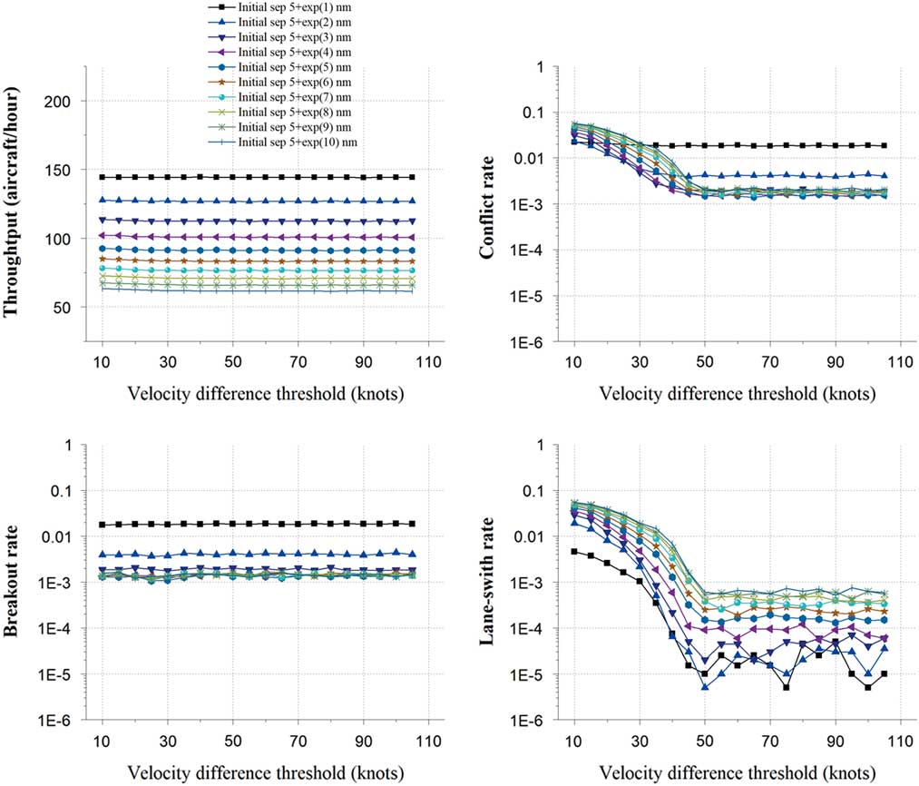
Figure 11 (Colour online) Initial separation and velocity difference threshold.

For the throughput, when the initial separation equals 5+exp (1) nm, the throughput achieves the maximum mean value of 144.21 aircraft/hour. As the initial separation increases to 5+exp (10) nm, the throughput stays at around 61.92 aircraft/hour.

For the conflict rate, when the initial separation equals 5+exp (1) nm, the conflict rate decreases to the minimum value of 0.0181 and then stays around 0.0185. When the initial separation equals 5+exp (10) nm, the conflict rate decreases to the minimum value of 0.0018 and then stays around 0.0021. The curves of breakout rate show no obvious changes with the increase of the velocity difference threshold. The breakout rate stays around 0.0183 when the initial separation equals 5+exp (1) nm, and decreases to around 0.0014 when the initial separation equals 5+exp (10). However, the curves of the lane-switch rate show a similar trend with the conflict rate. When the initial separation equals 5+exp (1) nm, the lane-switch rate decreases from 0.00458 to about 0.00005. When the initial separation equals 5+exp (10) nm, it decreases from 0.0546 to about 0.0006. A noticeable trend is that all the curves begin to stabilise when the velocity difference threshold reaching around 50 Kn.

These trends may indicate that the trigging condition for conflicts resolution will be harder with the increase of velocity difference threshold, leading to the decreases of breakout rates and lane-switch rates. Since the maximum difference of the standard cruise Mach numbers of the eight simulation aircraft types is 0.07 Mach (about 46.3 Kn), when the velocity difference threshold is larger than 50 Kn, few aircraft can trigger the lane-switch condition, so both the breakout rates and lane-switch rates reduce from that value.

4.3 Fractional factorial analysis

The quantitative impact of each parameter and the interaction between every pairwise combination of parameters could provide a better picture of how variations in the input parameters combine to affect the capacity and safety of flow corridor. Therefore, a fractional factorial analysis is conducted to study the interactions between self-separation parameters. Based on the sensitivity analysis results, each self-separation parameter is set to either its low value or high value as given in Table 7. All combinations of these values are studied. There are 2⁶=64 alternative experiments conducted in total, each with 10 replications and 100,000 simulated flights. From the outputs of these experiments, the main effects (impacts of single factors) and interaction effects (impacts of pairs of factors) are estimated. Because the input values are ‘normalised’ to either a low value or a high value, the resulting effects provide some measure of the relative impact of the parameters and their interactions. Of course, the results are somewhat dependent on the choice of the low and high values, and we choose the low and high value based on the sensitivity analysis above.

Table 7 Design of experiments, fractional factorial analysis

Figure 12 shows the main effects and interaction effects sorted by value. Both the corresponding parameter and the parameter pair are labelled on the y-axes. For the throughput, the dominating factor is initial separation which has a negative impact. It means that if the initial separation is increased, the throughput would decrease as expected. For the interaction effects of the parameter pair, the initial separation with the minimum separation and the separation buffer have similar positive impacts while the minimum separation from the separation buffer has a negative impact. For the conflict rate, the minimum separation, separation buffer and their interaction effects are the dominating factors which have major positive impacts, while the initial separation and its interaction effects with separation buffer and minimum separation have major negative impacts. The dominating factors of the breakout rate are similar to the conflict rate while the dominating factors of the lane-switch rate are the initial separation, velocity difference threshold and their interactions.

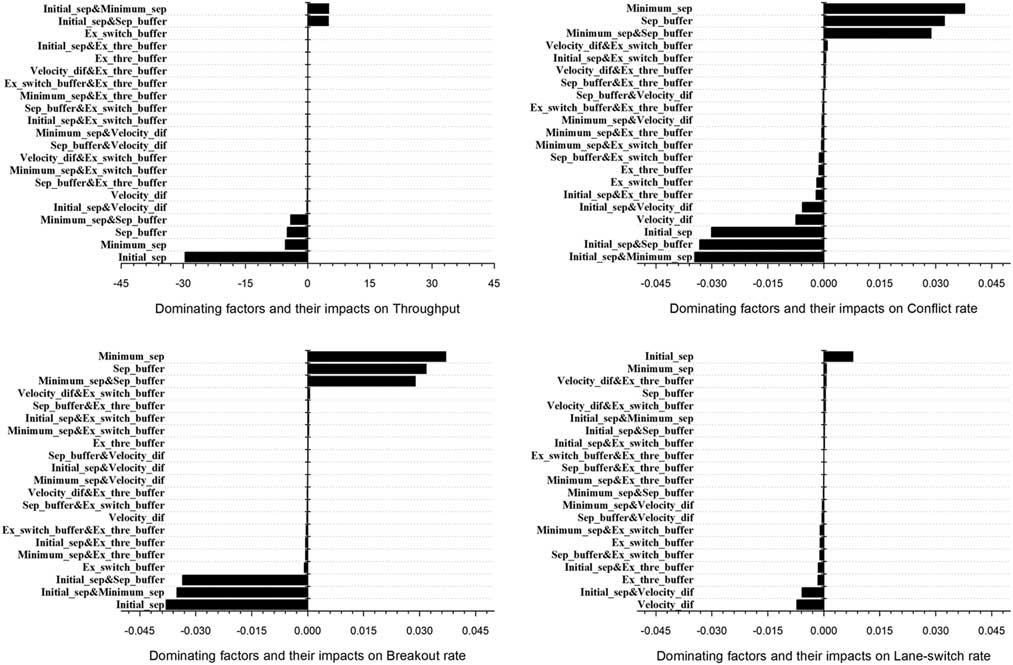
Figure 12 Full factorial ranking of effects for self-separation parameters.