


NOMENCLATURE
- a
speed of sound
- C p
specific heat at constant pressure
-
 ${ \hat{\rm F}}_{{c}} ,{\hat{\rm G}}_{{c}} ,{ \hat{\rm H}}_{{c}} $
convective (inviscid) flux vectors in generalised co-ordinates
-
${ \hat{\rm F}}_{{v}} ,{ \hat{\rm G}}_{{v}} ,{ \hat{\rm H}}_{{v}} $
viscous flux vectors in generalised co-ordinates
- H
enthalpy
- I
total numbers of reactions
- J
Jacobian of transformation matrix
- K
total number of species
- K e
reaction rate equilibrium constant
- k f
forward reaction rate
- k b
backward reaction rate
- M
Mach number
- p
pressure
-
${ \hat{\rm Q}}$
conservative vector of flow variables in generalised co-ordinates
-
${ \hat{\rm R}}$
residual vector
- R u
universal gas constant
- Re
Reynolds number
- S
entropy
-
${ \hat{\rm S}}$
chemical reaction source vector
- T
temperature
- U,V,W
contravariant velocity components
- ρ
density
- ξ,η,ζ
generalised co-ordinates
- τ
shear stress
-
$${\rm \nu }_{{k,i}}^{{\rm '}} ,{\rm \nu }_{{k,i}}^{{{\rm ''}}} $$
stoichiometric coefficients of the kth species in ith reaction
-
$\dot{\romega }$
source term (production term) for the chemical species
- χ
chemical symbol for the reactants and products


1.0 INTRODUCTION
In air-breathing propulsion systems for hypersonic flights, decelerating air from hypersonic to subsonic speeds increases the drag drastically. Therefore, in scramjets, one of the most promising air-breathing propulsive systems of hypersonic vehicles, combustion occurs at supersonic speeds( Reference Heiser, Pratt, Daley and Mehta 1 ). However, air entering the combustion chamber at supersonic speeds results in difficulties such as poor fuel–air mixing rate, reduced residence time and flame holding difficulty( Reference Segal 2 , Reference Smart 3 ). This makes the combustion chamber the most challenging part in the design of a scramjet engine.
Several methods have been introduced in order to overcome these difficulties. However, some of these methods introduce new issues. Obstacles in the flow path enhance the mixing and combustion efficiency by increasing the residence time. However, cooling these obstacles in high enthalpy flows causes severe heat transfer and material problems( Reference Baurle and Eklund 4 ). The pressure loss and drag increase due to the obstacles are the additional problems.
One of the methods to enhance the mixing in the combustor is to use ramp injectors. The purpose of ramp injectors is to increase the fuel–air mixing by adding fuel in the axial direction (i.e. injection of fuel parallel to the incoming flow direction)( Reference Dimotakis 5 ). This type of mechanism increases the mixing by producing counter-rotating vortices and creating shock and expansion waves as the supersonic flow passes over the ramps. Although ramp injectors enhance the fuel–air mixing and combustion efficiency, they possess some crucial disadvantages. Since the fuel is injected along the wall, mixing can only be enhanced near the wall until the shear layers expand into core flow at far downstream( Reference Segal 2 ). In addition, placing ramp injectors in flow path causes pressure losses and consequently an increase in drag( Reference Bonanos 6 ). Moreover, ramp injectors in high enthalpy flows produce high temperatures which can result in material degradation.
Struts can also be used to improve the mixing efficiency. Struts are placed vertically in the combustion chamber from bottom to top. Struts are designed with a wedge at the leading edge and fuel injectors at the trailing edge( Reference Pandey and Sivasakthivel 7 ). The mixing of fuel is better in configurations with struts because the fuel can be injected to flow field from several locations at the trailing edge. However, since struts are in-stream devices, they have large pressure losses and contribute significantly to the total drag( Reference Dessornes and Jourdren 8 ).
In the late 1990s, cavity flame holders were proposed as a new concept for flame stabilisation in supersonic combustion chambers( Reference Tishkoff, Drummond, Edwards and Nejad 9 ). The principle idea behind the cavity technique is to create a recirculation region where the mixing of the fuel and air occurs at relatively low speeds( Reference Wang, Wang and Sun 10 ). Since cavities are recessed in combustors, pressure losses are decreased compared to other techniques where the devices are placed in-stream. By creating low-speed recirculation regions, cavities increase the residence time and so, mixing and combustion become more efficient and stable. There are many factors affecting the performances of the cavity flame holders such as cavity geometry, fuel injection pattern and fuel type. A study by Hsu et al.( Reference Hsu, Goss and Roquemore 11 ) has shown that closed cavities result in unstable flames while open cavities with low aspect ratio do not provide enough volume for flame holding. Stable combustion can be achieved for a limited range of the length to depth ratio which corresponds to minimum drag and entrainment. Ben-Yakar( Reference Ben-Yakar 12 ) has demonstrated the effect of inclined cavity aft-wall on the reattachment of the shear layer and flame stabilisation. Experimental results show that for a cavity with a vertical aft-wall (i.e. no inclination in rear wall), compression waves propagate into the cavity. The propagation of waves into cavity occurs after the generation of shock waves in the shear layer reattachment location, at the cavity trailing edge. However, in the inclined cavities, the shear layer reattaches to the aft-wall in a steady manner so that no acoustic waves are reflected towards the inside of the cavity.
The flow field in scramjet combustors is quite complex. It involves shock interaction, fuel injection and heat release. In general, these complex phenomena are analysed by solving flow and chemical reaction equations together. Reviews of analysis models for scramjet combustors can be found in Refs Reference Baurle13–Reference Drummond15. Reynolds Averaged Navier–Stokes (RANS) equations, large Eddy simulations (LES) or direct numerical simulations (DNS) can be used for flow analyses( Reference Mura and Izard 16 – Reference Koo, Raman and Varghese 18 ). Among these, DNS is the most reliable model but is also computationally the most expensive one. Mostly, RANS or LES models are used in the flow analysis of scramjet combustors. While LES simulations are more accurate, the solutions of RANS are computationally multiple orders-of-magnitude more affordable than LES( Reference Arnold-Medabalimi and Duraisamy 19 ). Hence, RANS models are frequently used for the practical design applications of scramjet combustors. Different models can be utilised to analyse chemical reactions in scramjet combustors. Even though chemical equilibrium assumptions are frequently used in subsonic combustion, finite rate effects become more important in supersonic combustion because the time scales for fluid motion and chemical reactions may be in the same order of magnitude( Reference Cheng, Wehrmeyer, Pitz, Jarrett and Northam 20 ). Finite rate effects can be included in RANS and LES models using the species mass flux and source terms( Reference Baurle and Eklund 4 , Reference Berglund, Fedina, Fureby, Tegnér and Sabel’nikov 21 – Reference Lin, Tam, Jackson, Kennedy, Williams, Olmstead and Collatz 24 ). The implementation of turbulence models for chemically reacting supersonic flows is still a challenging research area. The laminar finite rate model ignores turbulence fluctuations in the calculation of species source term( Reference Berglund, Fedina, Fureby, Tegnér and Sabel’nikov 21 ). Although the model is exact for laminar flames, it may not be reliable for turbulent flames. In general, Reynolds averaging the source term requires a large number of unclosed correlations. This problem can be avoided using the probability density function (PDF) approach( Reference Mobus, Gerlinger and Bruggemann 25 – Reference Baurle and Girimajib 27 ). In PDF method, the reaction rates are modelled by using the presumed shape or transported probability density functions. Another approach to model the interactions between turbulence and chemistry is the flamelet technique. In this approach, the chemical time scale is assumed to be shorter than the turbulent time scale and the chemistry and turbulence calculations can be decoupled from each other( Reference Mura and Izard 16 , Reference Gao, Wang, Jiang and Lee 28 , Reference Li, Lou and Ladeinde 29 ). Although major advances have been achieved in developing new models to couple turbulence and chemistry, the improvements may not be very significant compared to the results evaluated from laminar chemistry and experimental data( Reference Choi, Ma and Yang 22 , Reference Mobus, Gerlinger and Bruggemann 25 ).
The simulation of chemically reacting flows requires the solution of a numerically stiff system of non-linear equations. The stiffness can be caused by the time scale differences in chemical reaction and flow equations. The chemical time scales may be orders of magnitude faster than the fluid dynamical time scales( Reference Leveque and Yee 30 ). Because of the numerical stability problems, step sizes in explicit methods are severely restricted. Hence, implicit methods are usually preferred for solving these equations. One of the important implicit algorithms for solving systems of non-linear equations is Newton’s method. Having quadratic convergence is the main advantage of Newton’s method. However, this is only possible if a good initial solution is supplied. Newton’s method requires the evaluation of Jacobian matrix that may be somewhat inconvenient and often tedious especially in the solutions of chemically reacting flows. In addition, solving and storing a large Jacobian matrix at each iteration may increase the CPU time and memory requirements, especially in large size problems. In order to keep the advantages and eliminate the disadvantages of Newton’s method, inexact Newton methods have been developed( Reference Dembo, Eisenstat and Steihaug 31 ). At each iteration of these methods, the Newton equation is solved approximately by using an efficient iterative solver. The JFNK method is one of the inexact Newton’s methods. As opposed to Newton’s method, the JFNK method does not require to explicitly form, store or solve any Jacobian matrices. In spite of having these advantages, the JFNK method has not been used to a large extent within the CFD community( Reference Chisholm and Zingg 32 ). This may be due to the fact that the efficiency of the JFNK method depends on several factors such as choosing the forcing term( Reference Eisenstat and Walker 33 ) and implementation of preconditioners( Reference Persson and Peraire 34 ). There are relatively few studies on solving chemically reacting flow equations using the JFNK method. Most of these studies are related to the analysis of low-speed combustors( Reference Knoll, Mchugh and Keyes 35 , Reference Mchugh, Knoll and Keyes 36 ). To the best of the authors’ knowledge, no literature is available concerning the implementation of the JFNK method for the analyses of high-speed scramjet combustors.
In the present study, a cavity type of scramjet combustor is analysed by solving the three-dimensional RANS and finite rate chemical reaction equations. In the solution of these coupled equations, the JFNK method is utilised. One of the objectives of this study is to evaluate the performance of the JFNK method in scramjet combustor analyses. For non-reactive and inviscid flow analyses of three-dimensional nozzles, a comparison of Newton’s and the JFNK methods is studied in Ref. Reference Yildizlar and Eyi37. Results show that the JFNK method is computationally more efficient, and the gap is getting wider in favour of the JFNK method as the grid size increases. Considering the increase in grid size in the solution of Navier–Stokes equations, it is not difficult to estimate that in the present scramjet combustor analyses, the JFNK method would be much more efficient compared to Newton’s method. Instead of comparing the JFNK method with other solution methods, the present study focuses on the parameters that affect the performance of the JFNK method in the analyses of scramjet combustors. The forcing term is one of the important parameters that determines the precision of the Newton correction term. The effect of the forcing term on the convergence behaviour of the JFNK method is evaluated in scramjet combustor analyses. Different flux splitting and limiter methods are utilised in the evaluation of inviscid and chemical species mass fluxes. The accuracy and convergence characteristics of these methods are compared in the analyses of a scramjet combustor. The developed CFD code is also used to analyse the effects of fuel injection angle on the mixing efficiency of scramjet combustor. The rest of the paper is organised as follows. In Section 2, the thermochemical modelling is introduced to analyse the chemically reacting supersonic flows. Computational modelling including the aerothermodynamic equations is described in Section 3. The implementation of the JFNK method is explained in Section 4. Results are discussed in Section 5 and the paper is concluded in Section 6.
2.0 THERMOCHEMICAL MODELING
At high temperatures, ideal gas equations may not be valid and the thermodynamic properties are evaluated using tables prepared from experimental data. In order to use these data for computational purposes, the experimental results are fit a polynomial equation. One of the widely used equations is the nine-constant polynomial form( Reference Mcbride, Zehe and Gordon 38 ), and it is the equation used in this study. In real gases, the following model is used to calculate the specific heat as a function of temperature:
 $${{C_{{p,k}}^{0} \left( T \right)} \over R}{\equals}a_{1} \,{1 \over {T^{2} }}{\plus}a_{2} \,{1 \over T}{\plus}a_{3} {\plus}a_{4} T{\plus}a_{5} T^{2} {\plus}a_{6} T^{3} {\plus}a_{7} T^{4} {\rm ,}$$
where a 1, a 2, …, a 7 are the coefficients of polynomial equations for different species( Reference Mcbride, Zehe and Gordon 38 ). For mixtures with K number of species, the specific heat at constant pressure is written as( Reference Yumuşak and Eyi 39 )
 $$C_{{{\rm pm}}} {\equals}\mathop \sum\limits_{k{\equals}1}^K {{{\rm \rrho }_{k} } \over {\rm \rrho }}{\rm }C_{{p,k}}^{0} {\rm }$$
The integration of polynomial for
 $C_{{p,k}}^{\rm 0} $
is employed to find the enthalpy for temperature T
$C_{{p,k}}^{\rm 0} $
is employed to find the enthalpy for temperature T
 $$H^{0} {\equals}{\int}_{T_{0} }^T {C_{p}^{0} {\rm d}T{\plus}B,} $$
where B is the constant of integration which makes the enthalpy zero at a reference temperature. The reference temperature and the pressure are defined as 298.15 K and 1 bar, respectively. For different temperatures, enthalpy is calculated as a sensible heat added to the heat of formation at the reference temperature( Reference Zehe, Gordon and Mcbride 40 )
 $$H^{0} (T){\equals}\Delta _{f} H^{0} (298.15){\plus}\left[ {H^{0} (T){\,\minus\,}H^{0} (298.15)} \right]$$
The polynomial to estimate the enthalpy is derived as follows:
 $${{H_{k}^{0} (T)} \over {RT}}{\equals}{\minus}a_{1} {\rm }{1 \over {T^{2} }}{\plus}a_{2} {\rm }{{{\rm ln }(T)} \over T}{\plus}a_{3} {\plus}a_{4} {T \over 2}{\plus}a_{5} {{T^{2} } \over 3}{\plus}a_{6} {{T^{3} } \over 4}{\plus}a_{7} {{T^{4} } \over 5}{\plus}{{b_{1} } \over T}{\rm }$$
In addition to the coefficients of a’s, the constants of integration, b 1, are needed for enthalpy calculations. The enthalpy of a mixture of species can be calculated as
 $$H_{m} {\equals}\mathop \sum\limits_{k{\equals}1}^K {{{\rm \rrho }_{k} } \over {\rm \rrho }}{\rm }H_{k}^{0} {\rm }$$
In order to evaluate the polynomial for entropy change, the specific heat at constant pressure is divided by temperature and then integrated. The integration bounds from the reference temperature to the local temperature
 $$S^{0} {\equals}{\int}_{T_{0} }^T {{{C_{p}^{0} } \over T}{\rm d}T{\plus}C} {\rm }$$
The polynomial for entropy is found as
 $${{S_{k}^{0} (T)} \over R}{\equals}{\minus}a_{1} {\rm }{1 \over {2T^{2} }}{\minus}a_{2} {\rm }{1 \over T}{\plus}a_{3}\ {\rm ln}T{\plus}a_{4} T{\plus}a_{5} {{T^{2} } \over 2}{\plus}a_{6} {{T^{3} } \over 3}{\plus}a_{7} {{T^{4} } \over 4}{\plus}b_{2} {\rm }$$
Similarly, the constants of integration, b 2, are defined for entropy calculations. The entropy of a mixture can also be evaluated as
 $$S_{m} {\equals}\mathop \sum\limits_{k{\equals}1}^K {{{\rm \rrho }_{k} } \over {\rm \rrho }}{\rm }S_{k}^{0} {\rm }$$
The value of internal energy for different species can be calculated as
 $$E_{k}^{\rm 0} {\equals}H_{k}^{0} {\minus}RT{\rm }$$
The specific internal energy can be estimated by using the mass fraction of different species
 $$e{\equals}\mathop \sum\limits_{k{\equals}1}^K {\rm }{{{\rm \rrho }_{k} } \over {\rm \rrho }}{\rm }E_{k}^{0} {\rm }$$
2.1 Finite rate chemical reaction model
In finite rate chemistry models, the system of chemical reaction equations for the K number of species and I number of reactions is written as follows:
 $$\mathop \sum\limits_{k{\equals}1}^K \nu _{{k,i}}^{\prime} {\rm \chi }_{k} {\rm }\,{\rightarrow{\hskip-14pt\vskip-4pt\leftarrow}\,}{\rm }\mathop \sum\limits_{k{\equals}1}^K \nu _{{k,i}}^{{{\rm ''}}} {\rm \rchi }_{k} {\rm ,}$$
where
 $\nu _{{k,i}}^{'} $
and
$\nu _{{k,i}}^{'} $
and
 $\nu _{{k,i}}^{\prime\prime} $
show the stoichiometric coefficient of the kth species in the ith reaction for the reactants and products, respectively. In the equation above, χ
k
is the chemical symbol for the kth species. The Arrhenius expression to calculate the forward reaction rate is given in the following equation:
$\nu _{{k,i}}^{\prime\prime} $
show the stoichiometric coefficient of the kth species in the ith reaction for the reactants and products, respectively. In the equation above, χ
k
is the chemical symbol for the kth species. The Arrhenius expression to calculate the forward reaction rate is given in the following equation:
 $$k_{{f,i}} {\equals}A_{i} T^{{B_{i} }} {\rm exp}\left( {{\minus}{{E_{i} } \over {R_{u} T}}} \right){\rm ,}$$
where A i is the rate of reaction constant, B i is the temperature exponent and E i is the activation energy for the ith reaction. The Arrhenius type of relation can also be used for reverse reaction rate calculations if these constants are available for reverse reactions. Otherwise, the backward reaction rate constant can be evaluated using the equilibrium constant given below
 $$K_{{e,i}} {\equals}\left( {{{p_{{{\rm atm}}} } \over {RT}}} \right)^{{\mathop{\sum}\limits_{k{\equals}1}^K {^{{{\rm \nu }_{{k,i}}^{{{\rm ''}}} {\minus}{\rm \nu }_{{k,i}}^{{\rm '}} }} } }} {\rm }\,{\rm exp }\left( {\mathop \sum\limits_{k{\equals}1}^K (\nu _{{k,i}}^{{{\rm ''}}} {\minus}\nu _{{k,i}}^{{\rm '}} )\left[ {{{S_{k} } \over R}{\minus}{{H_{k} } \over {RT}}} \right]} \right){\rm }$$
In this case, the backward reaction rate is related to the forward reaction rate and equilibrium constant according to
 $$k_{{b,i}} {\equals}{{k_{{f,i}} } \over {K_{{e,i}} }}{\rm }$$
The production of the kth species is evaluated as follows:
 $${\dot {\rm \romega }}_{k} {\equals}W_{k} {\rm }\mathop \sum\limits_{k{\equals}1}^K \left( {{\rm \nu }_{{k,i}}^{\rm ''} {\minus}{\rm \nu }_{{k,i}}^{\prime} } \right)\,\left( {k_{{fi}} \,\mathop \prod\limits_{k{\equals}1}^K \left[ {{\rm \rchi }_{k} } \right]^{{{\rm \nu }_{{k,i}}^{\prime} }} {\minus}k_{{bi}} \mathop {\,\prod}\limits_{k{\equals}1}^K \left[ {{\rm \rchi }_{k} } \right]^{{{\rm \nu }_{{k,i}}^{\prime\prime} }} } \right){\rm }$$
where [χ k ] is the molar concentration and W k is the molecular weight of kth species.
2.2 Ethylene–air combustion model
Throughout the years, several fuels have been tested for scramjets. Among these, hydrogen and hydrocarbon fuels are used extensively. Fry( Reference Fry 41 ) shows that hydrogen fuels are more beneficial for flight Mach numbers above 8. On the other hand, hydrocarbon fuels may be preferred for flight Mach numbers below 8. Hydrocarbon fuels are advantageous because of high density (requiring less volume), easy storage (not highly reactive) and more energy content per volume( Reference Lewis 42 ). However, hydrocarbon fuels also have the disadvantages of slow reaction and long ignition delay time( Reference Powell, Edwards, Norris, Numbers and Pearce 43 ). In this study, the scramjet is considered for low hypersonic flows (Mach numbers below 8), and hence, ethylene (C2H4) is employed as fuel.
Hydrocarbon fuels with large carbon compositions in their molecules have extensive reaction mechanisms, and solving these systems requires high computation time and effort. Therefore, reduced ethylene reaction mechanisms are necessary considering the computational efficiency. In the study by Baurle and Eklund( Reference Baurle and Eklund 4 ), the reaction mechanism is reduced to three steps by adjusting the reactions rate for the absence of hydroxyl, which decreases the ignition delay time( Reference Eklund, Baurle and Gruber 44 ). In the present study, this reduced finite rate chemical reaction model is used for ethylene ignition with three reactions and six species as it is shown in Table 1.
Table 1 Forward reaction rate data for reduced ethylene–air combustion( Reference Baurle and Eklund 4 )

3.0 COMPUTATIONAL MODELING
The coupled equations of Navier–Stokes and finite rate chemical reactions are solved to analyse the flow inside the scramjet combustor. In order to ease the implementation of boundary conditions, the computational space is transformed from Cartesian co-ordinates to generalised co-ordinates. Different flux splitting methods with the first- and second-order discretisation are employed. Discretised equations are solved using the JFNK method.
The non-dimensional form of the three-dimensional Navier–Stokes and finite rate chemical reaction equations in generalised co-ordinates can be written as
 $${{\partial ({ \hat{\rm F}}_{c} {\minus}{ \hat{\rm F}}_{v} )} \over {\partial {\rm \rxi }}}{\plus}{{\partial ({ \hat{\rm G}}_{c} {\minus}{ \hat{\rm G}}_{v} )} \over {\partial {\rm \reta }}}{\plus}{{\partial ({ \hat{\rm H}}_{c} {\minus}{ \hat{\rm H}}_{v} )} \over {\partial {\rm \rzeta }}}{\minus}{ \hat{\rm S}}{\equals}0{\rm }$$
In the equation above, inviscid flux vectors can be expressed as
 $${ \hat{\rm F}}_{c} {\equals}{1 \over J}{\rm }\left[ {\matrix{ {{\rm \rrho }U} \cr {{\rm \rrho }Uu{\plus}{\rm \rxi }_{x} p} \cr {{\rm \rrho }Uv{\plus}{\rm \rxi }_{y} p} \cr {{\rm \rrho }Uw{\plus}{\rm \rxi }_{z} p} \cr {\left( {{\rm \rrho }e_{t} {\plus}p} \right)U} \cr {{\rm \rrho }_{1} U} \cr \vdots \cr {{\rm \rrho }_{{K{\minus}1}} U} \cr } } \right]{\rm ,}{ \,\hat{\rm G}}_{c} {\equals}{1 \over J}{\rm }\left[ {\matrix{ {{\rm \rrho }V} \cr {{\rm \rrho }Vu{\plus}{\rm \reta }_{x} p} \cr {{\rm \rrho }Vv{\plus}{\rm \reta }_{y} p} \cr {{\rm \rrho }Vw{\plus}{\rm \reta }_{z} p} \cr {\left( {{\rm \rrho }e_{t} {\plus}p} \right)V} \cr {{\rm \rrho }_{1} V} \cr \vdots \cr {{\rm \rrho }_{{K{\minus}1}} V} \cr } } \right]{\rm ,}\,{ \hat{\rm H}}_{c} {\equals}{1 \over J}{\rm }\left[ {\matrix{ {{\rm \rrho }W} \cr {{\rm \rrho }Wu{\plus}{\rm \rzeta }_{x} p} \cr {{\rm \rrho }Wv{\plus}{\rm \rzeta }_{y} p} \cr {{\rm \rrho }Ww{\plus}{\rm \rzeta }_{z} p} \cr {\left( {{\rm \rrho }e_{t} {\plus}p} \right)W} \cr {{\rm \rrho }_{1} W} \cr \vdots \cr {{\rm \rrho }_{{K{\minus}1}} W} \cr } } \right]{\rm ,}$$
where contravariant velocities are defined as
 $$U{\equals}{\rm \rxi }_{x} u{\plus}{\rm \rxi }_{y} v{\plus}{\rm \rxi }_{z} w,\quad V{\equals}{\rm \reta }_{x} u{\plus}{\rm \reta }_{y} v{\plus}{\rm \reta }_{z} w,\quad W{\equals}{\rm \rzeta }_{x} u{\plus}{\rm \rzeta }_{y} v{\plus}{\rm \rzeta }_{z} w{\rm }$$
As shown in Equation (18), chemical species mass fluxes are included in inviscid flux vectors.
 $\hat{S}$
is the production (source) vector for chemical species. Similarly, viscous flux vectors are written as
$\hat{S}$
is the production (source) vector for chemical species. Similarly, viscous flux vectors are written as
 $$\eqalignno{ & { \hat{\rm F}}_{v} {\equals}{1 \over J}{\rm }\left[ {\matrix{ 0 \cr {{\rm \rxi }_{x} {\rm \rtau }_{{xx}} {\;\plus\;}{\rm \rxi }_{y} {\rm \rtau }_{{xy}} {\;\plus\;}{\rm \rxi }_{z} {\rm \rtau }_{{xz}} } \cr {{\rm \rxi }_{x} {\rm \rtau }_{{xy}} {\;\plus\;}{\rm \rxi }_{y} {\rm \rtau }_{{yy}} {\;\plus\;}{\rm \rxi }_{z} {\rm \rtau }_{{yz}} } \cr {{\rm \rxi }_{x} {\rm \rtau }_{{xz}} {\;\plus\;}{\rm \rxi }_{y} {\rm \rtau }_{{yz}} {\;\plus\;}{\rm \rxi }_{z} {\rm \rtau }_{{zz}} } \cr {{\rm \rxi }_{x} b_{x} {\;\plus\;}{\rm \rxi }_{y} b_{y} {\;\plus\;}{\rm \rxi }_{z} b_{z} } \cr 0 \cr \vdots \cr 0 \cr } } \right]{\rm },\,{ \hat{\rm G}}_{v} {\equals}\left[ {\matrix{ 0 \cr {{\rm \reta }_{x} {\rm \rtau }_{{xx}} {\;\plus\;}{\rm \reta }_{y} {\rm \rtau }_{{xy}} {\;\plus\;}{\rm \reta }_{z} {\rm \rtau }_{{xz}} } \cr {{\rm \reta }_{x} {\rm \rtau }_{{xy}} {\;\plus\;}{\rm \reta }_{y} {\rm \rtau }_{{yy}} {\;\plus\;}{\rm \reta }_{z} {\rm \rtau }_{{yz}} } \cr {{\rm \reta }_{x} {\rm \rtau }_{{xz}} {\;\plus\;}{\rm \reta }_{y} {\rm \rtau }_{{yz}} {\;\plus\;}{\rm \reta }_{z} {\rm \rtau }_{{zz}} } \cr {{\rm \reta }_{x} b_{x} {\;\plus\;}{\rm \reta }_{y} b_{y} {\;\plus\;}{\rm \reta }_{z} b_{z} } \cr 0 \cr \vdots \cr 0 \cr } } \right] \cr & { \hat{\rm H}}_{v} {\equals}\left[ {\matrix{ 0 \cr {{\rm \rzeta }_{x} {\rm \rtau }_{{xx}} {\plus}{\rm \rzeta }_{y} {\rm \rtau }_{{xy}} {\plus}{\rm \rzeta }_{z} {\rm \rtau }_{{xz}} } \cr {{\rm \rzeta }_{x} {\rm \rtau }_{{xy}} {\plus}{\rm \rzeta }_{y} {\rm \rtau }_{{yy}} {\plus}{\rm \rzeta }_{z} {\rm \rtau }_{{yz}} } \cr {{\rm \rzeta }_{x} {\rm \rtau }_{{xz}} {\plus}{\rm \rzeta }_{y} {\rm \rtau }_{{yz}} {\plus}{\rm \rzeta }_{z} {\rm \rtau }_{{zz}} } \cr {{\rm \rzeta }_{x} b_{x} {\plus}{\rm \rzeta }_{y} b_{y} {\plus}{\rm \rzeta }_{z} b_{z} } \cr 0 \cr \vdots \cr 0 \cr } } \right]{\rm ,}\,{ \hat{\rm S}}{\equals}\left[ {\matrix{ 0 \cr 0 \cr 0 \cr 0 \cr 0 \cr {{\dot{\romega }}_{1} } \cr \vdots \cr {{\dot{\romega }}_{{K{\minus}1}} } \cr } } \right]{\rm ,} $$
where
 $$\eqalignno{ b_{x} & {\equals}ut_{{xx}} {\plus}vt_{{xy}} {\plus} wt_{{xz}} {\plus}kT_{x} ,\quad b_{y} {\equals}ut_{{xy}} {\plus}vt_{{yy}} {\plus}wt_{{yz}} {\plus}kT_{y} \cr b_{z} & {\equals}u\rtau _{{xz}} {\plus}v\rtau _{{yz}} {\plus}w\rtau _{{zz}} {\plus}kT_{z} $$
In the equation above, k is the thermal conductivity and T is the temperature. The shear stresses in the equation above can be written in tensor notation as follows:
 $${\rm \rtau }_{{x_{i} x_{j} }} {\equals}\left[ {{\rm \rmu }\left( {{{\partial u_{i} } \over {\partial x_{j} }}{\plus}{{\partial u_{j} } \over {\partial x_{i} }}} \right){\plus}\lambda {{\partial u_{k} } \over {\partial x_{k} }}{\rm \delta }_{{ij}} } \right],$$
where λ is the bulk viscosity which is related to the dynamic viscosity, μ (calculated as a function of temperature using the power law, with a power of unity) by the Stokes hypothesis as in the equation below:
 $${\rm \rlambda }{\equals}{\minus}{2 \over 3}{\rm \rmu }$$
The equations above include the momentum diffusion due to viscosity and the energy diffusion due to thermal conductivity. The mass diffusion due to species concentration is not included. In the present study, the non-dimensional form of the Navier–Stokes and finite rate reaction equations are solved using the non-dimensional Mach, Reynolds and Prandtl numbers.
Moreover, the Spalart–Allmaras (S–A) one equation turbulence model( Reference Spalart and Allmaras 45 ) is implemented for eddy viscosity calculations. The S–A model solves the kinematic eddy turbulent viscosity which is modelled by the following transport equation:
 $${{\partial {\tilde{\nu }}} \over {\partial t}}{\plus}\tilde{u}_{j} {{\partial {\tilde{\nu }}} \over {\partial x_{j} }}{\equals}c_{{b1}} \tilde{S}{\tilde{\nu }}{\plus}{1 \over \sigma }\left[ {{\partial \over {\partial x_{j} }}\left( {\left( {{\rm \nu }{\plus}{\tilde{\nu }}} \right){\plus}{{\partial {\tilde{\nu }}} \over {\partial x_{j} }}} \right){\plus}c_{{b2}} {{\partial {\tilde{\nu }}} \over {\partial x_{j} }}{{\partial {\tilde{\nu }}} \over {\partial x_{j} }}} \right]{\minus}c_{{{\rm \romega }1}} f_{{\rm \romega }} \left( {{{{\tilde{\nu }}} \over d}} \right)^{2} $$
and, turbulent eddy viscosity is given as
 $${\rm \rmu }_{t} {\equals}{\rm \bar{\rho }}\tilde{\nu }f_{{\nu 1}} {\equals}{\rm \bar{\rho }\nu }_{t} $$
where
 $\tilde{S}$
is the vorticity magnitude, σ is the turbulent Prandtl number and f
ω
is a non-dimensional function. Similarly, d is the distance from the wall and c
b1, c
b2 and c
ω1 are the constants. Since Reynolds averaging the source term requires a large number of unclosed correlations, the laminar finite rate model is utilised in the present study; the effects of turbulence fluctuations on the chemical species source term are ignored(
Reference Baurle and Girimajib
27
).
$\tilde{S}$
is the vorticity magnitude, σ is the turbulent Prandtl number and f
ω
is a non-dimensional function. Similarly, d is the distance from the wall and c
b1, c
b2 and c
ω1 are the constants. Since Reynolds averaging the source term requires a large number of unclosed correlations, the laminar finite rate model is utilised in the present study; the effects of turbulence fluctuations on the chemical species source term are ignored(
Reference Baurle and Girimajib
27
).
3.1 Flux vector splitting
The governing equations presented in generalised co-ordinates in Equation (17) can be discretised as
 $${{{\rm \delta }_{{\rm \rxi }} ({ \hat{\rm F}}_{c} {\minus}{ \hat{\rm F}}_{v} )} \over {\Delta {\rm \rxi }}}{\plus}{{{\rm \delta }_{{\rm \reta }} ({ \hat{\rm G}}_{c} {\minus}{ \hat{\rm G}}_{v} )} \over {\Delta {\rm \reta }}}{\plus}{{{\rm \delta }_{{\rm \rzeta }} ({ \hat{\rm H}}_{c} {\minus}{ \hat{\rm H}}_{v} )} \over {\Delta {\rm \rzeta }}}{\minus}{ \hat{\rm S}}{\equals}0$$
For a cell-cantered finite volume method, Equation (26) becomes
 $$\eqalignno{ & \left( {{ \hat{\rm F}}_{c} {\minus}{ \hat{\rm F}}_{v} } \right)_{{i{\plus}{1 \over 2},{\rm }j,{\rm }k}} {\minus}\left( {{ \hat{\rm F}}_{c} {\minus}{ \hat{\rm F}}_{v} } \right)_{{i{\minus}{1 \over 2},{\rm }j,{\rm }k}} {\plus}\left( {{ \hat{\rm G}}_{c} {\minus}{ \hat{\rm G}}_{v} } \right)_{{i,{\rm }j{\plus}{1 \over 2},{\rm }k}} {\minus}\left( {{ \hat{\rm G}}_{c} {\minus}{ \hat{\rm G}}_{v} } \right)_{{i,{\rm }j{\minus}{1 \over 2},{\rm }k}} \cr & \quad \quad {\plus}\left( {{ \hat{\rm H}}_{c} {\minus}{ \hat{\rm H}}_{v} } \right)_{{i,{\rm }j,{\rm }k{\plus}{1 \over 2}}} {\minus}\left( {{ \hat{\rm H}}_{c} {\minus}{ \hat{\rm H}}_{v} } \right)_{{i,{\rm }j,{\rm }k{\minus}{1 \over 2}}} {\minus}{ \hat{\rm S}}_{{i,j,k}} {\equals}0 $$
where the i±1/2, j±1/2 and k±1/2 denote cell interfaces.
In this study, upwind flux splitting schemes are used for the spatial discretisation of the flux vectors:
 $$\eqalignno{ & \left[ {{ \hat{\rm F}}_{c}^{{\plus}} \left( {{ \hat{\rm Q}}^{{\minus}} } \right)_{{i{\plus}{1 \over 2},{\rm }j,{\rm }k}} {\plus}{ \hat{\rm F}}_{c}^{{\minus}} \left( {{ \hat{\rm Q}}^{{\plus}} } \right)_{{i{\plus}{1 \over 2},{\rm }j,{\rm }k}} } \right]{\minus}\left[ {{ \hat{\rm F}}_{c}^{{\plus}} \left( {{ \hat{\rm Q}}^{{\minus}} } \right)_{{i{\minus}{1 \over 2},{\rm }j,{\rm }k}} {\plus}{ \hat{\rm F}}_{c}^{{\minus}} \left( {{ \hat{\rm Q}}^{{\plus}} } \right)_{{i{\minus}{1 \over 2},{\rm }j,{\rm }k}} } \right] \cr & {\plus}\left[ {{ \hat{\rm G}}_{c}^{{\plus}} \left( {{ \hat{\rm Q}}^{{\minus}} } \right)_{{i,{\rm }j{\plus}{1 \over 2},{\rm }k}} {\plus}{ \hat{\rm G}}_{c}^{{\minus}} \left( {{ \hat{\rm Q}}^{{\plus}} } \right)_{{i,{\rm }j{\plus}{1 \over 2},{\rm }k}} } \right]{\minus}\left[ {{ \hat{\rm G}}_{c}^{{\plus}} \left( {{ \hat{\rm Q}}^{{\minus}} } \right)_{{i,{\rm }j{\minus}{1 \over 2},{\rm }k}} {\plus}{ \hat{\rm G}}_{c}^{{\minus}} \left( {{ \hat{\rm Q}}^{{\plus}} } \right)_{{i,{\rm }j{\minus}{1 \over 2},{\rm }k}} } \right] \cr & {\plus}\left[ {{ \hat{\rm H}}_{c}^{{\plus}} \left( {{ \hat{\rm Q}}^{{\minus}} } \right)_{{i,{\rm }j,{\rm }k{\plus}{1 \over 2}}} {\plus}{ \hat{\rm H}}_{c}^{{\minus}} \left( {{ \hat{\rm Q}}^{{\plus}} } \right)_{{i,{\rm }j,{\rm }k{\plus}{1 \over 2}}} } \right]{\minus}\left[ {{ \hat{\rm H}}_{c}^{{\plus}} \left( {{ \hat{\rm Q}}^{{\minus}} } \right)_{{i,{\rm }j,{\rm }k{\minus}{1 \over 2}}} {\plus}{ \hat{\rm H}}_{c}^{{\minus}} \left( {{ \hat{\rm Q}}^{{\plus}} } \right)_{{i,{\rm }j,{\rm }k{\minus}{1 \over 2}}} } \right]{\minus}{ \hat{\rm S}}_{{i,j,k}} {\equals}0 $$
There are several methods for splitting flux vectors. Steger–Warming, van Leer and AUSM schemes are some of the most widely used flux vector splitting methods which are implemented in this study.
The Steger–Warming scheme is one of the first flux vector splitting methods(
Reference Steger and Warming
46
). In this method, the flux vector is split according to the sign of the eigenvalues of Jacobian matrix. The split fluxes in ξ-direction can be given in the following equation and the split fluxes in other directions (
 $\hat{\rm G}_c} {^}{\!\!\!^\pm\,} $
and
$\hat{\rm G}_c} {^}{\!\!\!^\pm\,} $
and
 $ \hat {\rm H}_{c}^{\!\pm\,} $
) can be evaluated similarly
$ \hat {\rm H}_{c}^{\!\pm\,} $
) can be evaluated similarly
 $${ \hat{\rm F}}_{c}^{\!\pm\,} {\equals}{{\rm \rrho } \over {2{\rm \rgamma }}}{\rm }\left[ {\matrix{ {\rm \rbeta } \cr {{\rm \rbeta }u{\plus}a\left( {{\rm \rlambda }_{2}^{\!\!\pm\,} {\minus\;}{\rm \rlambda }_{3}^{\!\!\pm\!} } \right){\hat{\rm \rxi }}_{x} } \cr {{\rm \rbeta }v{\plus}a\left( {{\rm \rlambda }_{2}^{\!\!\pm\,} {\minus\;}{\rm \rlambda }_{3}^{\!\!\pm\!} } \right){\hat{\rm \rxi }}_{y} } \cr {{\rm \rbeta }w{\plus}a\left( {{\rm \rlambda }_{2}^{\!\!\pm\,} {\minus\;}{\rm \rlambda }_{3}^{\!\!\pm\!} } \right){\hat{\rm \rxi }}_{z} } \cr {{\rm \rbeta }{{\left( {u^{2} {\plus}v^{2} {\plus}w^{2} } \right)} \over 2}{\plus}aU_{{\rm \rxi }} \left( {{\rm \rlambda }_{2}^{\!\!\pm\,} {\minus\;}{\rm \rlambda }_{3}^{\!\!\pm\!} } \right){\plus}{{a^{2} \left( {{\rm \rlambda }_{2}^{\!\!\pm\,} {\minus\;}{\rm \rlambda }_{3}^{\!\!\pm\!} } \right)} \over {{\rm \rgamma }{\,\minus}1}}} \cr {{\rm \rbeta }({\rm \rrho }_{1}/{\rm \rrho })} \cr \vdots \cr {{\rm \rbeta }({\rm \rrho }_{{K{\minus}1}}/{\rm \rrho })} \cr } } \right],$$
where
 $$\eqalignno{ & {\rm \rbeta }{\equals}2\left( {{\rm \rgamma }{\minus}1} \right){\rm \rlambda }_{1}^{\!\!\pm\,} {\plus}{\rm \rlambda }_{2}^{\!\!\pm\,} {\plus}{\rm \rlambda }_{3}^{\!\!\pm\,} \cr & \vskip8pt {\hat{\rm \rxi }}_{i} {\equals}{{{\rm \rxi }_{i} } \over {\sqrt {{\rm \rxi }_{x}^{2} {\plus}{\rm \rxi }_{y}^{2} {\plus}{\rm \rxi }_{z}^{2} } }} $$
 $${\hat{\rm \reta }}_{i} {\equals}{{{\rm \reta }_{i} } \over {\sqrt {{\rm \reta }_{x}^{2} {\plus}{\rm \reta }_{y}^{2} {\plus}{\rm \reta }_{z}^{2} } }}{\rm ,}\quad {\hat{\rm \rzeta }}_{i} {\equals}{{{\rm \rzeta }_{i} } \over {\sqrt {{\rm \rzeta }_{x}^{2} {\plus}{\rm \rzeta }_{y}^{2} {\plus}{\rm \rzeta }_{z}^{2} } }}{\rm }$$
In the following equations, the contravariant velocities,
 ${\hat{\rm U}}$
, are defined using the direction cosines of
${\hat{\rm U}}$
, are defined using the direction cosines of
 ${\hat{\rm \rxi }}_{x} , {\hat{\rm \rxi }}_{y} , {\hat{\rm \rxi }}_{z} , {\hat{\rm \reta }}_{x} , \,\ldots\,,{\hat{\rm \rzeta }}_{z} $
:
${\hat{\rm \rxi }}_{x} , {\hat{\rm \rxi }}_{y} , {\hat{\rm \rxi }}_{z} , {\hat{\rm \reta }}_{x} , \,\ldots\,,{\hat{\rm \rzeta }}_{z} $
:
 $${\hat{\rm U}}_{\rxi } {\equals}u{\hat{\rm \rxi }}_{x} {\plus}v{\hat{\rm \rxi }}_{y} {\plus}w{\hat{\rm \rxi }}_{z} $$
 $${\hat{\rm U}}_{{\rm \reta }} {\equals}u{\hat{\rm \reta }}_{x} {\plus}v{\hat{\rm \reta }}_{y} {\plus}w{\hat{\rm \reta }}_{z} {\rm ,}\quad {\hat{\rm U}}_{\rzeta } {\equals}u{\hat{\rm \rzeta }}_{x} {\plus}v{\hat{\rm \rzeta }}_{y} {\plus}w{\hat{\rm \rzeta }}_{z} $$
van Leer( Reference Van Leer 47 ) introduced a new upwind flux vector splitting method that uses the Mach number for splitting the flux vector. In this method, the flux vectors are discretised separately for subsonic and supersonic regions. In supersonic regions, the original flux vector is used. In subsonic regions, the flux vector in ξ-direction can be written as
 $${ \hat{\rm F}}_{c}^{\!\pm\,} {\equals}\,\pm{{{\rm \rrho }a} \over J}\left( {{{M\,\pm\,1} \over 2}} \right)^{2} \left[ {\matrix{ 1 \cr {{1 \over {\rm \rgamma }}\left( {{\minus}{\hat{\rm U}}_{{\rm \rxi }} \,\pm\,2a} \right){\hat{\rm \rxi }}_{x} {\plus}u} \cr {{1 \over {\rm \rgamma }}\left( {{\minus}{\hat{\rm U}}_{{\rm \rxi }} \,\pm\,2a} \right){\hat{\rm \rxi }}_{y} {\plus}u} \cr {{1 \over {\rm \rgamma }}\left( {{\minus}{\hat{\rm U}}_{{\rm \rxi }} \,\pm\,2a} \right){\hat{\rm \rxi }}_{z} {\plus}u} \cr {{{{\hat{\rm U}}_{{\rm \rxi }} \left( {{\minus}{\hat{\rm U}}_{{\rm \rxi }} \,\pm\,2a} \right)} \over {{\rm \rgamma }{\plus}1}}{\plus}{{2a} \over {{\rm \rgamma }^{2} {\minus}1}}{\plus}{{u^{2} {\plus}v^{2} {\plus}w^{2} } \over 2}} \cr {{\rm \rrho }_{1}/{\rm \rrho }} \cr \vdots \cr {{\rm \rrho }_{{K{\minus}1}} /{\rm \rrho }} \cr } } \right]$$
where J is the Jacobian Matrix, a is the speed of sound and γ is the specific heat ratio.
Another flux vector splitting method used in this study is Advection Upstream Splitting Method (AUSM) which is a rather new method suggested by Liou and Steffen( Reference Liou and Steffen 48 ). Although, in principle, it is similar to the van Leer method, the AUSM is based on convection and pressure splitting. Similar to the van Leer splitting, the original flux vectors can be used in supersonic regions. However, in subsonic regions, the pressure is split according to the following equation:
 $$p^{\pm\,} {\equals}{\rm }{1 \over 2}p\left( {1\,\pm\,M} \right){\rm }$$
In subsonic regions, the split flux vector by AUSM method can be written in ξ-direction (
 $\hat{F}_{c}^{\!\pm\,} $
) as follows:
$\hat{F}_{c}^{\!\pm\,} $
) as follows:
 $${ \hat{\rm F}}_{c}^{\!\pm\,} {\equals}\,\pm{1 \over J}\left( {{{M\,\pm\,1} \over 2}} \right)^{2} \left[ {\matrix{ {{\rm \rrho }a} \cr {{\rm \rrho }a{\plus}u{\hat{\rm \rxi }}_{x} p^{\!\pm\,} } \cr {{\rm \rrho }a{\plus}v{\hat{\rm \rxi }}_{y} p^{\!\pm\,} } \cr {{\rm \rrho }a{\plus}w{\hat{\rm \rxi }}_{z} p^{\!\pm\,} } \cr {a\left[ {{\rm \rrho }e_{t} {\plus}\left( {{\rm \rgamma }{\minus}1} \right)\left( {{\rm \rrho }e{\minus}{{u^{2} {\plus}v^{2} {\plus}w^{2} } \over 2}} \right)} \right]{\rm }} \cr {{\rm \rrho }a({\rm \rrho }_{1} /{\rm \rrho })} \cr \vdots \cr {{\rm \rrho }a({\rm \rrho }_{{K{\minus}1}} /{\rm \rrho })} \cr } } \right]$$
3.2 Order of accuracy
In first-order schemes, flow variables at cell interfaces are evaluated from the left and right neighbouring cell centres. Simply, the left and right flow variables at cell interfaces in i direction can be written as
 $${ \hat{\rm Q}}_{{i{\plus}{1 \over 2},j,k}}^{{\minus}} {\equals}{ \hat{\rm Q}}_{{i,j,k}} ,\quad { \hat{\rm Q}}_{{i{\plus}{1 \over 2},j,k}}^{{\plus}} {\equals}{ \hat{\rm Q}}_{{i{\plus}1,j,k}} {\rm }$$
In second-order schemes, the information of the flow variables at cell interfaces are computed by interpolating the flow variable values from neighbouring cells. By increasing the order of interpolation, higher order schemes can be constructed. In second-order schemes, the left and right flow variables at cell interface can be evaluated using the Monotonic Upstream-Cantered scheme for Conservation Laws (MUSCL) scheme:( Reference Van Leer 47 )
 $$\eqalignno{ & Q_{{i{\plus}{1 \over 2},j,k}}^{{\minus}} {\equals}Q_{{i,j,k}} {\plus}{1 \over 4}\left[ {\left( {1{\minus}\kappa } \right)a_{{i,j,k}} {\plus}\left( {1{\plus}\kappa } \right)b_{{i,j,k}} } \right] \cr & Q_{{i{\plus}{1 \over 2},j,k}}^{{\plus}} {\equals}Q_{{i{\plus}1,j,k}} {\minus}{1 \over 4}\left[ {\left( {1{\minus}\kappa } \right)b_{{i{\plus}1,j,k}} {\plus}\left( {1{\plus}\kappa } \right)a_{{i{\plus}1,j,k}} } \right] $$
where
 $$a_{{i,j,k}} {\equals}Q_{{i,j,k}} {\minus}Q_{{i{\minus}1,j,k}} ,\quad {\rm }b_{{i,j,k}} {\equals}Q_{{i{\plus}1,j,k}} {\minus}Q_{{i,j,k}} $$
In the equation above, κ has a value between −1 and 1 and defines the spatial accuracy of discretisation. A third-order scheme is formed for the value of 1/3. For other values, a second-order scheme is evaluated.
Constructing higher order schemes improves the accuracy of the solutions. However, higher order schemes may produce artificial oscillations in high gradient regions. In order to avoid these problems, flux limiter functions can be employed to identify the high gradient regions in the flow domain and reduce the accuracy to first order in these regions. In this way, oscillations can be prevented. The second-order schemes with flux limiters are constructed as in the following equations:
 $$\eqalignno{ & Q_{{i{\plus}{1 \over 2},j,k}}^{{\minus}} {\equals} Q_{{i,j,k}} {\plus}{{{\rm \rpsi }(r_{{i,j,k}} )} \over 4}\left[ {\left( {1{\minus}\kappa } \right)a_{{i,j,k}} {\plus}\left( {1{\plus}\kappa } \right)b_{{i,j,k}} } \right] \cr & Q_{{i{\plus}{1 \over 2},j,k}}^{{\plus}} {\equals}Q_{{i{\plus}1,j,k}} {\minus}{{{\rm \rpsi }(r_{{i{\plus}1,j,k}} )} \over 4}\left[ {\left( {1{\minus}\kappa } \right)b_{{i{\plus}1,j,k}} {\plus}\left( {1{\plus}\kappa } \right)a_{{i{\plus}1,j,k}} } \right] $$
where r i,j,k is given by the following equation:
 $$r_{{i,j,k}} {\equals}{{b_{{i,j,k}} } \over {a_{{i,j,k}} }}$$
In Equation (39), ψ is a flux limiter function, and can be evaluated in several ways. In this study, the flux limiter functions of Min-mod, Superbee, van Leer and van Albada are employed and defined as follows:
Min-mod:
 $${\rm \rpsi (}r{\rm )}{\equals}\max \left[ {0,{\rm min(}1,r{\rm )}} \right]$$
Superbee:
 $${\rm \rpsi (}r{\rm )}{\equals}\max \left[ {0,{\rm min}\left( {2r,1} \right),{\rm min}(r,2)} \right]$$
van Leer:
 $${\rm \rpsi (}r{\rm )}{\equals}{{r{\plus}\left| r \right|} \over {1{\plus}\left| r \right|}}$$
van Albada:
 $${\rm \rpsi (}r{\rm )}{\equals}{{r^{2} {\plus}r} \over {r^{2} {\plus}1}}$$
Among these functions, the method introduced by van Albada is most used. Venkatakrishnan( Reference Venkatakrishnan 49 ) suggested the following modified version of van Albada to improve the convergence characteristics of the second-order schemes:
 $$\eqalignno{ & {\rm \rpsi }\left( {r_{i} } \right){\equals}{{a_{i} \left( {b_{i}^{2} {\plus}{\rm {\repsilon}}^{2} } \right){\plus}b_{i} \left( {a_{i}^{2} {\plus}{\rm {\repsilon}}^{2} } \right)} \over {a_{i}^{2} {\plus}b_{i}^{2} {\plus}2{\rm {\repsilon}}^{2} }}\quad {\rm for \;\rkappa }{\equals}0 \cr & {\rm \rpsi }\left( {r_{i} } \right){\equals}{{a_{i} \left( {2b_{i}^{2} {\plus}{\rm {\repsilon}}^{2} } \right){\plus}b_{i} \left( {a_{i}^{2} {\plus}2{\rm {\repsilon}}^{2} } \right)} \over {a_{i}^{2} {\plus}b_{i}^{2} {\minus}a_{i} b_{i} {\plus}3{\rm {\repsilon}}^{2} }}{\rm }\quad {\rm for \;\rkappa }{\equals}{1 \over 3} $$
where ε is a parameter to reduce the effects of the flux limiter in smooth flow regions to increase the convergence characteristics of the scheme.
4.0 JFNK METHOD
In this study, the three-dimensional Navier–Stokes and finite rate chemical reaction equations are coupled and solved using the JFNK method which is one of the inexact Newton’s methods that utilises a Krylov subspace approach( Reference Yildizlar and Eyi 37 , Reference Saad and Schultz 50 ). The main goal of the Krylov subspace method is to solve a system of linear equations, Ax=b. Starting from the initial solution of x, after each iteration, a new solution is found along with the correction in the Krylov subspace. The JFNK method is matrix-free, in other words, the Jacobian matrix is not computed. Only a matrix vector multiplication is needed which is done through the directional or Frechet derivative approach. In other words, to calculate the solution, the process does not need to access to entries of the matrix A.
The mathematical representation of the JFNK method is given as follows. The residual vector,
 ${ \hat{\rm R}}({ \hat{\rm Q}})$
, for the three-dimensional Navier–Stokes and finite rate chemical reaction equations can be written in the following form:
${ \hat{\rm R}}({ \hat{\rm Q}})$
, for the three-dimensional Navier–Stokes and finite rate chemical reaction equations can be written in the following form:
 $${ \hat{\rm R}}({ \hat{\rm Q}}){\equals}{{\partial ({ \hat{\rm F}}_{c} {\minus}{ \hat{\rm F}}_{v} )} \over {\partial {\rm \rxi }}}{\plus}{{\partial ({ \hat{\rm G}}_{c} {\minus}{ \hat{\rm G}}_{v} )} \over {\partial {\rm \reta }}}{\plus}{{\partial ({ \hat{\rm H}}_{c} {\minus}{ \hat{\rm H}}_{v} )} \over {\partial {\rm \rzeta }}}{\minus}{ \hat{\rm S}}{\equals}0$$
The goal in Newton’s method is to approach zero residual at the next iteration. Newton’s method can be formulated as in the following equation
 $$\eqalignno{ & \left( {{{\partial { \hat{\rm R}}} \over {\partial { \hat{\rm Q}}}}} \right)_{k} \Delta { \hat{\rm Q}}_{k} {\equals}{\minus}{ \hat{\rm R}}({ \hat{\rm Q}}_{k} ) \cr & { \hat{\rm Q}}_{{k{\plus}1}} {\equals}{ \hat{\rm Q}}_{k} {\plus}\Delta { \hat{\rm Q}}_{k} , $$
where
 ${ \hat{\rm Q}}_{{k{\plus}1}} $
denotes the value of
${ \hat{\rm Q}}_{{k{\plus}1}} $
denotes the value of
 ${ \hat{\rm Q}}$
at the next iteration and
${ \hat{\rm Q}}$
at the next iteration and
 $\partial { \hat{\rm R}}/\partial { \hat{\rm Q}}$
is the Jacobian matrix which needs to be solved in Newton’s methods. In the JFNK algorithm, Newton’s method is approximately solved. The accuracy of the approximate solution is controlled by a forcing term η
k
which ranges from zero to one. Convergence characteristics of the JFNK method are highly dependent on the value of the η
k
. The implementation of this term in the calculation of the residual can be expressed as
$\partial { \hat{\rm R}}/\partial { \hat{\rm Q}}$
is the Jacobian matrix which needs to be solved in Newton’s methods. In the JFNK algorithm, Newton’s method is approximately solved. The accuracy of the approximate solution is controlled by a forcing term η
k
which ranges from zero to one. Convergence characteristics of the JFNK method are highly dependent on the value of the η
k
. The implementation of this term in the calculation of the residual can be expressed as
 $$\left\Vert {{ \hat{\rm R}}\left( {{ \hat{\rm Q}}_{k} } \right){\plus}{ \hat{\rm R}}{'} \left( {{ \hat{\rm Q}}_{k} } \right) \Delta { \hat{\rm Q}}_{k} \right\Vert {\leq {\rm \reta }_{k} } \right\Vert{ \hat{\rm R}}({ \hat{\rm Q}}_{k} )} \right\Vert$$
Although in Newton’s method, the Jacobian matrix,
 ${ \hat{\rm R}}{'} \left( {{ \hat{\rm Q}}} \right)$
, is needed to find the flow variables at the next iteration, in the JFNK method, the multiplication of the Jacobian matrix with a vector, v, is approximated as follows(
Reference Knoll and Keyes
51
):
${ \hat{\rm R}}{'} \left( {{ \hat{\rm Q}}} \right)$
, is needed to find the flow variables at the next iteration, in the JFNK method, the multiplication of the Jacobian matrix with a vector, v, is approximated as follows(
Reference Knoll and Keyes
51
):
 $${ \hat{\rm R}}{'} \left( {{ \hat{\rm Q}}} \right)\! \cdot\! v\,\approx\, {{{ \hat{\rm R}}\left( {{ \hat{\rm Q}}{\plus}\!\!\in \!v} \right){\minus}{ \hat{\rm R}}\left( {{ \hat{\rm Q}}} \right)} \over \in}$$
Therefore, the computation of the Jacobian matrix is not necessary and this method is referred to as matrix-free numerical solution algorithm. The JFNK method shown in the following algorithm is utilised in the present study( Reference Yildizlar and Eyi 37 ).
Algorithm 1. JFNK method

5.0 RESULTS
The geometry of the scramjet combustion chamber used in this study is identical to one used in the experimental scramjet tested in Wright–Patterson Air Force Base( Reference Lin, Tam, Jackson, Kennedy, Williams, Olmstead and Collatz 24 ), which is one of the most recent and commonly used experimental scramjet engines. Data from the experimental studies for this scramjet are available in the literature which are crucial for code validation purposes. The schematic of the full experimental scramjet engine is shown in Fig. 1.
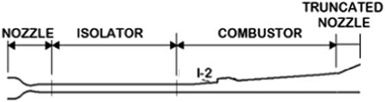
Figure 1 Schematic of the experimental scramjet( Reference Lin, Tam, Jackson, Kennedy, Williams, Olmstead and Collatz 24 ).
In the experimental facility, the nozzle provides high-speed flow to the isolator. The isolator separates the inlet from the combustor and compresses the air through a set of oblique shocks. In the combustor section, air mixes with fuel which is injected from the I-2 injector. The truncated nozzle is placed to accelerate the flow behind the scramjet. The combustion chamber of this experimental scramjet is designed with a cavity recessed in its body wall. The wall has a constant divergence angle of 2.6° and the cavity has a length to depth ratio of 5. Moreover, the aft-wall of the cavity has an angle of 22.5° with respect to the cavity floor. The size of the cavity-based combustor is shown in Fig. 2. The configuration of the fuel injectors used in the scramjet combustion chamber is shown in Fig. 3. In order to take the advantage of recirculation region around the cavity, fuel is injected from the upstream of the cavity.
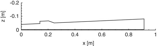
Figure 2 Two-dimensional drawing of the combustor.

Figure 3 Upstream fuel injection configuration (top view).
The location of the fuel injectors is important in increasing the mixing efficiency. In this study, the reactant of the fuel (ethylene) is oxygen. Fuel injectors located far upstream may cause flame holding problems because of the high velocities at the combustor entrance. High-speed flow in the combustion chamber reduces the residence time and may result in low mixing efficiency. Because of the low residence time, flames may be unstable and continuous combustion would not occur. On the other hand, if the fuel injectors were placed on the leading edge of the cavity, the fuel may not be able to penetrate into the core flow. In this situation, the shear layer interrupts the fuel–air mixing and so the efficiency of the mixing may significantly decrease. Therefore, the fuel should be injected from a small distance upstream of the cavity leading edge. In this way, higher mixing efficiency of fuel–air may be achieved in the cavity region. This is one of the important characteristics of the cavities which make them more efficient compared with other flame holding methods in scramjet combustors.
In the following sections, first, the convergence of the JFNK method is studied in the analysis of the scramjet combustor. Then, a grid independent study is performed and results are compared with experimental data. Later, the analysis results with the first- and second-order schemes are presented. Finally, the reaction mechanism is analysed and the change of the mixing efficiency with fuel injection angle is presented.
5.1 Convergence of the JFNK method
As mentioned earlier, the convergence of the JFNK method may be degraded in the solution of chemically reactive flow equations. Since species flux calculations utilise inviscid flux splitting methods, first, the effects of different flux vector splitting schemes on the convergence of the JFNK method are studied. Next, in the flow analyses of a supersonic combustor, the effects of the first- and second-order methods on the convergence behaviours of the JFNK method are studied. In second-order methods, different flux limiters are evaluated and their performance is compared. Finally, the influences of the forcing term on convergence behaviours of the JFNK method are studied. In order to evaluate the pure effects of chemical species flux evaluation on the convergence of the JFNK method, viscous fluxes are not activated. In all other flow analyses, viscous fluxes are activated. A convergence criterion is defined; iterations are stopped when the norm value of residual is reduced six orders of magnitude from initial values.
5.1.1 Effects flux splitting schemes
In scramjet combustor flow analyses, the effects of different flux splitting methods on the convergence of the JFNK method are studied. Steger–Warming, van Leer and AUSM methods are employed to calculate the inviscid and chemical species mass fluxes. In Fig. 4, the convergence histories with different splitting methods are shown for the first-order schemes. Steger–Warming method reaches the convergence criteria about 1,700 outer iterations, whereas van Leer and AUSM methods meet the same criteria in less than 1,200 outer iterations. In other words, van Leer and AUSM flux splitting methods show a better performance compared to Steger–Warming method for the first-order scheme. In the JFNK method, every outer iteration contains inner iterations. Hence, the CPU time becomes more important for the convergence characteristics. The CPU times to reach the specified residual tolerance are tabulated in Table 2. Even though the AUSM scheme reaches convergence criteria at a higher iteration number, the CPU time in the AUSM scheme is lower. This shows that the van Leer method has larger inner steps at every iteration. Among these methods, the Steger–Warming method shows the worst characteristic considering both the iteration number and the CPU time.

Figure 4 Convergence of JFNK method with different flux splitting methods (first-order schemes).
Table 2 CPU times of JFNK method with different flux splitting methods (first-order schemes)

5.1.2 Effects of the order of schemes
In the flow analyses of the scramjet combustor, the effects of the order of accuracy on the convergence of the JFNK method are studied. In first-order flux splitting schemes, the values at cell centres are used directly as cell face values. In these schemes, the variation of flow variables between cell centres and cell faces is neglected. However, in second-order flux splitting schemes, the flow variables at cell interfaces are calculated by using the interpolation between the variables at cell centre; the variation of the values between the cell centres and faces is taken into account. Therefore, second-order schemes are expected to give more accurate solutions than first-order schemes. Both the first- and second-order schemes are implemented using Steger–Warming, van Leer and AUSM flux vector splitting methods.
The convergence histories of the first- and second-order schemes with Steger–Warming, AUSM and van Leer flux splitting methods are shown in Fig. 5. Initially, no limiters are implemented for second-order schemes to realise the pure effects of the order of schemes on the convergence of the JFNK method. In the next section, the comparison is extended to include the limiters effects. The solution of the first-order schemes meets the convergence criteria using a lower number of iterations, while the second-order schemes experience oscillations. Although second-order schemes are expected to give more accurate solutions, first-order schemes are computationally more efficient. The comparison of Tables 2 and 3 shows that to reach the same convergence level, the CPU times of second-order schemes are approximately seven times longer compared with first-order schemes.
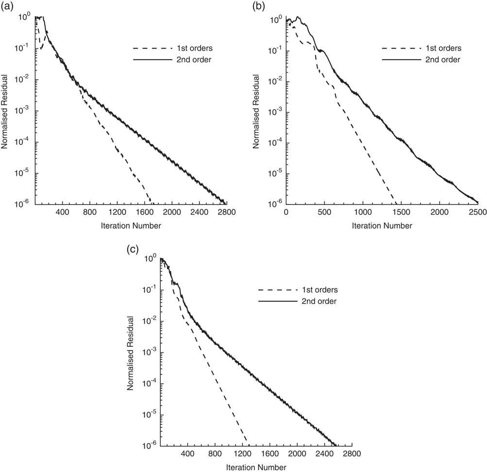
Figure 5 Converge of JFNK method with first- and second-order schemes. (a) Steger-Warming; (b) AUSM; and (c) van Leer.
Table 3 CPU times of JFNK method with second-order schemes

5.1.3 Effects of the flux limiters
Using high-order schemes for flows with discontinuities may cause oscillations in the solution domain. In order to eliminate these oscillations flux limiters are generally used. van Albada, Min-Mod, Superbee and van Leer limiters are implemented using the second-order van Leer flux splitting method. The effects of these limiters on the convergence of the JFNK method are studied in the analyses of the scramjet combustor. Figure 6 shows that the van Albada flux limiter function (both second- and third-order accuracies) has a better convergence history. The van Albada limiter of third-order accuracy provides the best convergence by reaching the normalised residual criteria in less than 1,400 iterations. Comparing Figs 5 and 6 shows that using flux limiters improves the convergence characteristics. As seen in Fig. 6, applying flux limiters also decreases the fluctuations in the residual history.
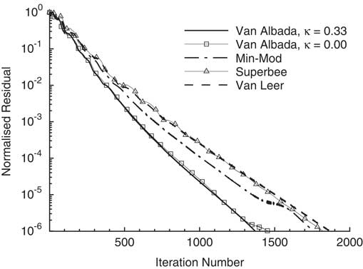
Figure 6 Effects of limiters on convergence of JFNK method.
5.1.4 Effects of the forcing term
The forcing term, η k , is one of the important parameters that influences the performance of the JFNK method. The effects of the forcing terms on the convergence of the JFNK method are studied in the analyses of the scramjet combustor. Although different strategies have been developed for the evaluation of the forcing term( Reference Eisenstat and Walker 33 ), the constant values are generally utilised( Reference Chisholm and Zingg 32 ), as in the present study. Figure 7 and Table 4 show the convergence of the JFNK method with different values of the forcing term. For flux splitting, the van Leer method is implemented with both the first- and the second-order of accuracy.
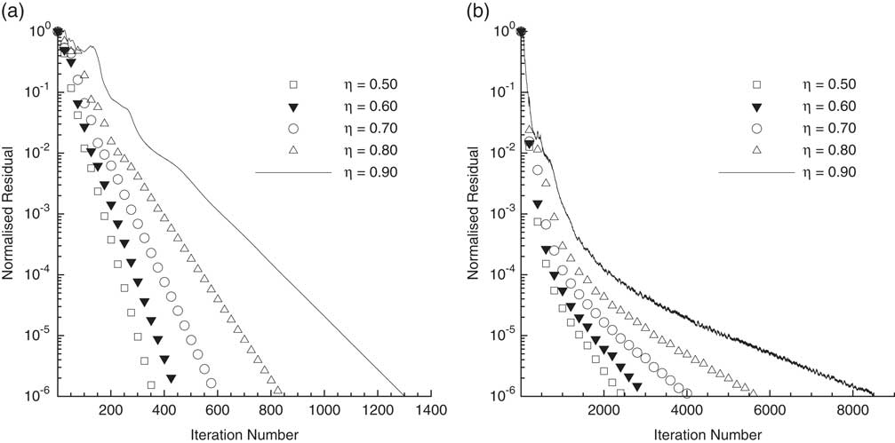
Figure 7 Effects of forcing term on convergence of JFNK method. (a) First and (b) second orders.
Table 4 Variation of CPU time for different forcing terms

As expected, the larger values of the forcing terms increase the deviations from the exact Newton’s method, and hence increase the number of outer iterations. As mentioned earlier, the CPU time is a more important convergence criterion in the JFNK method. Table 4 shows that increasing the forcing term value decreases the CPU time in both the first- and second-order schemes. However, in first-order schemes, increasing the forcing term value beyond 0.80 degrades the convergence. Thus, using the forcing term values between 0.8 and 0.9 generally gives the best convergence characteristics in scramjet combustor analyses.
5.2 Grid independent study
A mesh refinement study is performed in order to realise the sensitivity of the solutions to grid resolution. Three different mesh levels are used and categorised as coarse, medium and fine. The number of nodes for each grid resolution is given in Table 5. Although using a finer grid resolution improves the accuracy, the CPU time required to achieve this accuracy may also increase. Therefore, the goal is to reach the best possible accuracy in the solution with as low resolution as possible.
Table 5 Generated meshes with different resolutions

In steady state analyses, a symmetry boundary condition can be implemented at the combustor’s half span. Although this approach is valid and reduces the computational cost significantly, it might lead to physically unreasonable results for unsteady simulations. Since the present study involves only steady-state analyses, equations are solved in half of the domain. The medium mesh is shown in Fig. 8 for the whole domain.
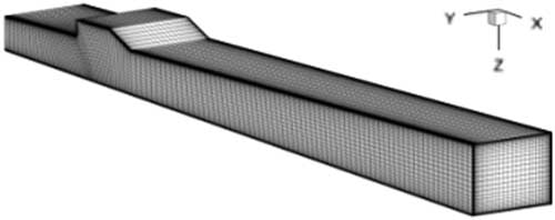
Figure 8 Medium grid size generated for viscous flows.
The developed code is validated with the experimental data by Lin et al.( Reference Lin, Tam, Jackson, Kennedy, Williams, Olmstead and Collatz 24 ). Moreover, the numerical solutions given in the same reference are also used for validation. The experiments are done to simulate the flight conditions of Mach 4.5. At this condition, the Mach number of 2.2 and the total temperature of 950 K are reached at the isolator inlet. In their flow analyses, a commercial code (CFD++), is utilised to solve RANS equations with the two-equation cubic κ−ε turbulence model. In Fig. 9, the solutions with different grid resolutions are compared with the experimental and computational data given in Ref. Reference Lin, Tam, Jackson, Kennedy, Williams, Olmstead and Collatz24. In the present study, the Prandtl number is 0.72, the Reynolds number with respect to combustor’s length is set to 105 and the fuel to air ratio is set to 0.02. Although discrepancies in pressure increase downstream of the cavity, considering the computational data in Ref. Reference Lin, Tam, Jackson, Kennedy, Williams, Olmstead and Collatz24, the results from the present study are generally in good agreement with the experimental data. Pressure distributions are getting close to the experimental data as the grid resolution is increased. The pressure distribution obtained for the coarse mesh deviates more from the experimental data. Having very similar solutions with the medium and fine meshes implies that, in this case, mesh dependency of the solution becomes insignificant from the medium to the fine mesh. However, the CPU time for the fine mesh is much higher (Table 6). Therefore, in this study, the solutions are evaluated using the medium mesh size.
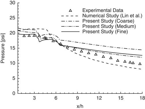
Figure 9 Comparison of pressure distribution with experimental and numerical data.
Table 6 Variation of CPU time for different grid resolutions

The three-dimensional variations of density, pressure, temperature and Mach number through the combustion chamber are shown in Fig. 10. In order to visualise the details of three-dimensional contours, half of the domain starting from the symmetry plane are shown. In addition to flow properties, variations in the mass fraction of the species are shown in Fig. 11. The effects of the cavity placement in the combustor can be clearly seen from the figures; the chemical reactions occur mostly in the cavity region.
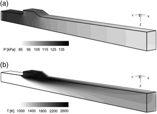
Figure 10 Pressure (a) and temperature (b) variations (second-order scheme).
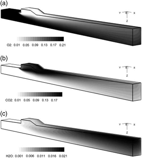
Figure 11 Species mass fraction variations (second-order scheme). (a) Oxygen mass fraction; (b) carbon dioxide mass fraction and (c) dihydrogen monoxide mass fraction.
5.3 Comparison of first- and second-order schemes
The scramjet combustor is analysed by solving the three-dimensional Navier–Stokes and finite rate chemical reaction equations. The Spalart–Allmaras model is utilised for turbulence closure. Fluxes are evaluated using the van Leer splitting and the van Albada limiter is utilised for the second-order scheme. The solutions from the first- and second-order splitting methods are compared. For this purpose, the variations of different flow variables and species’ mass fractions are plotted in the cavity region of the combustor. The cavity region is the most important part of the combustor because of the discontinuities in the geometry and high gradients in flow. The cavity region is shown in Fig. 12.
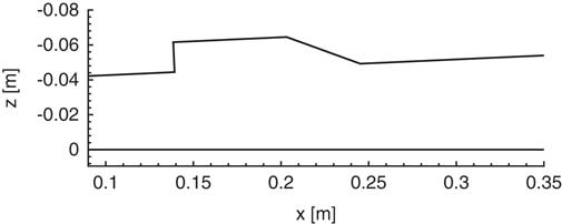
Figure 12 Cavity section of the combustor.
First, two-dimensional variations of flow variables and species’ mass fractions are studied. The variations perpendicular to wall are plotted at different streamwise locations. In Fig. 13, these variations in the cavity region are compared for the first- and second-order schemes. Results show that the variations of flow variables are sharper in the second-order scheme. In other words, the second-order scheme can capture the abrupt changes due to flow discontinuities. Moving away from the wall boundaries into the core flow, the discrepancies between the first- and second-order schemes become larger. Generally, in the second-order scheme, a detailed variation of the flow variables is obtained. However, these variations are quite smooth in the first-order scheme.
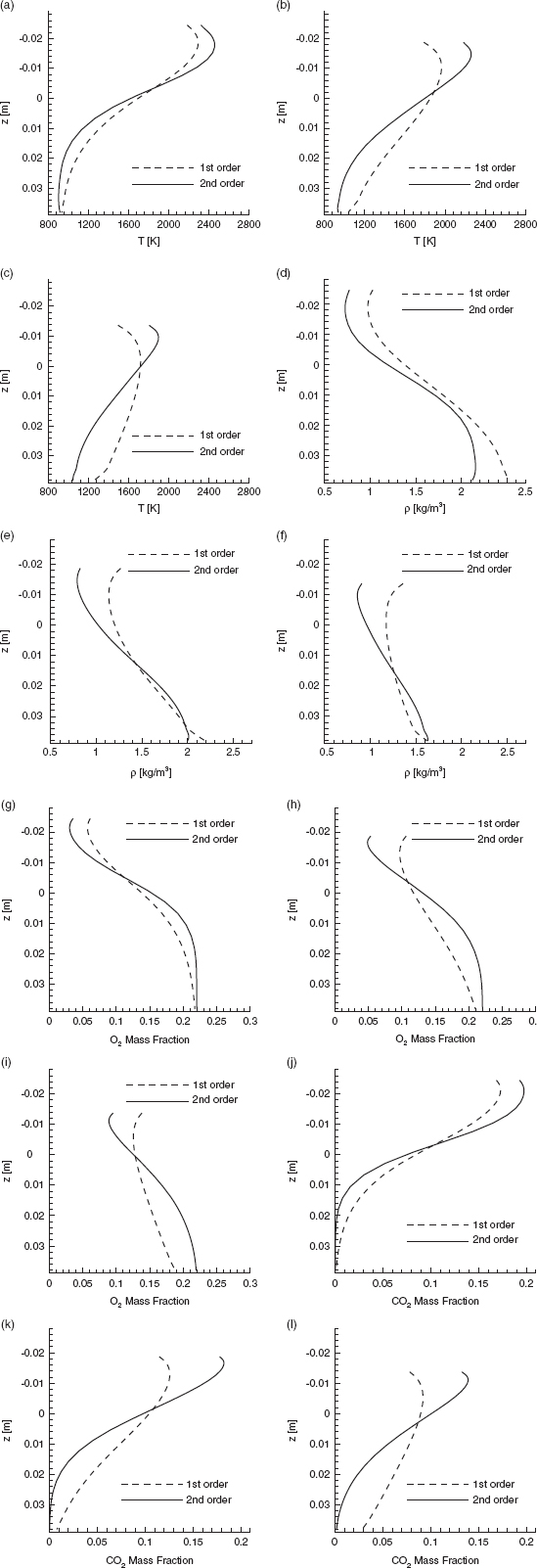
Figure 13 Two-dimensional distribution of flow variables at different axial locations. Temperature at (a) x = 0.17 m; (b) x = 0.23 m; and (c) x = 0.31 m. Density at (d) x = 0.17 m; (e) x = 0.23 m; and (f) x = 0.31 m. Oxygen at (g) x = 0.17 m; (h) x = 0.23 m; and (i) x = 0.31 m. Carbon dioxide at (j) x = 0.17 m; (k) x = 0.23 m; and (l) x = 0.31 m.
Next, the three-dimensional variations of flow variables and species’ mass fractions are compared for the first- and second-order schemes. In Fig. 14, solutions are shown on the symmetry plane of the combustor. Results show that the second-order scheme presents detailed information about the flow properties and chemical species. Small changes in flow variables are more distinguishable in the second-order scheme. The solutions from the first- and second-order schemes are rather similar in low gradient regions. In the scramjet combustion chamber, the cavity creates a 90° deflection angle in geometry and the fuel injection causes a sudden change in flow variables and species concentration. Considering all these, the second-order scheme is preferred in the flow analysis of combustors.
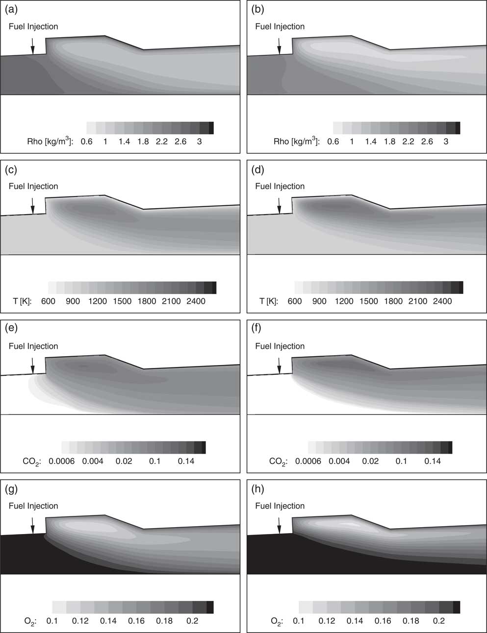
Figure 14 Comparison of first- and second-order schemes by contour. Density ((a) first and (b) second orders). Temperature ((c) first and (d) second orders). Carbon dioxide mass fraction ((e) first and (f) second orders). Oxygen mass fraction ((g) first and (h) second orders).
5.4 Reaction mechanism analysis
The temperature and the mixing efficiency variations are the two important parameters for combustor performance. In this study, the mixing efficiency of the reaction mechanism is defined as( Reference Baurle and Eklund 4 , Reference Powell, Edwards, Norris, Numbers and Pearce 43 )
 $${\rm \reta }_{m} {\equals}{{{\int} {Y_{r} {\rm \rrho (}{\mib{\rm v}} .{\mib{\rm n}} {\rm )d}A} } \over {{\int} {Y{\rm \rrho (}{\mib{\rm v}} .{\mib{\rm n}} {\rm )d}A} }}$$
In the equation above, Y is defined as the mass fractions of fuel (for globally fuel lean cases) or the oxidant (for globally fuel-rich cases). Similarly, Y r is the mass fraction of the least available reactant (based on the global equivalence ratio). One-dimensional mass flux weighted values of temperature and mixing efficiency are calculated from their three-dimensional distributions. The fuel is injected approximately 0.1 m downstream of the combustor inlet. As shown in Fig. 15, starting from the fuel injection location, both temperature and mixing efficiency rise, although the increase in mixing efficiency is sharper. The delay in temperature increase may be related to having high flow velocity and insufficient reaction time near the injector. In finite rate chemistry models, reactions can be completed in a finite time interval and distance. One-dimensional mass flux weighted values of species’ mass fractions are studied in Fig. 16. After the injection of fuel, chemical reactions take place between ethylene and oxygen; carbon monoxide and hydrogen are produced. Results show that the mass fraction of oxygen reduces after the fuel injection. In addition, the increase in the mass fraction of hydrogen stops and then it continuously drops downstream of the cavity. This is reasonable since the produced hydrogen reacts with oxygen to give dihydrogen monoxide (water) as a product. Therefore, the production of dihydrogen monoxide continuously increases toward combustor exit.

Figure 15 Variation of mass flux-weighted temperature (a) and mixing efficiency (b).
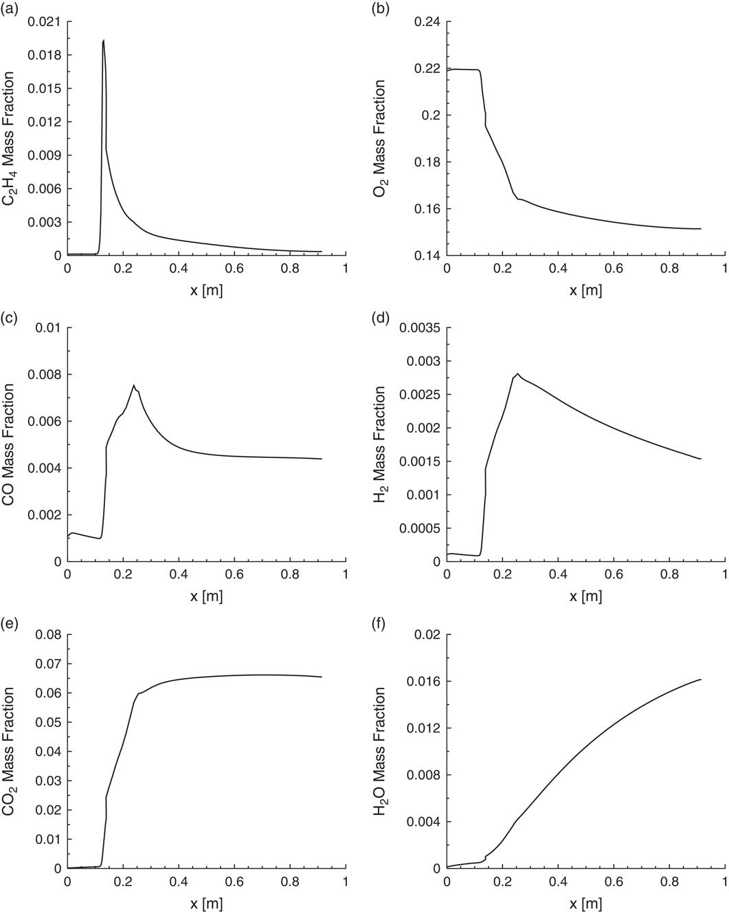
Figure 16 Mass flux weighted 1D variation of species through combustor. (a) Ethylene; (b) oxygen; (c) carbon monoxide; (d) hydrogen; (e) carbon dioxide; and (f) dihydrogen monoxide.
5.5 Effects of fuel injection angle
Because of the low residence time of the flow in the combustion chamber, fuel–air mixing becomes a crucial problem. In addition to using cavities to increase the mixing efficiency, other methods can also be employed to increase the fuel–air mixing efficiency even further. Injecting fuel at different angles changes the penetration of fuel to the core flow and consequently the mixing efficiency. The present study evaluates the effectiveness of this phenomena. Two cases are examined. In the first case, fuel is injected in the flow direction with different angles. Figure 17(a) shows the change of mixing efficiencies with respect to the injection angle in the axial direction. In general, very high (near 90°) or very low (near 15°) fuel injection angles decrease the mixing efficiency. The maximum mixing efficiency is approximately 80% and it is achieved for a fuel injection angle of 60°.
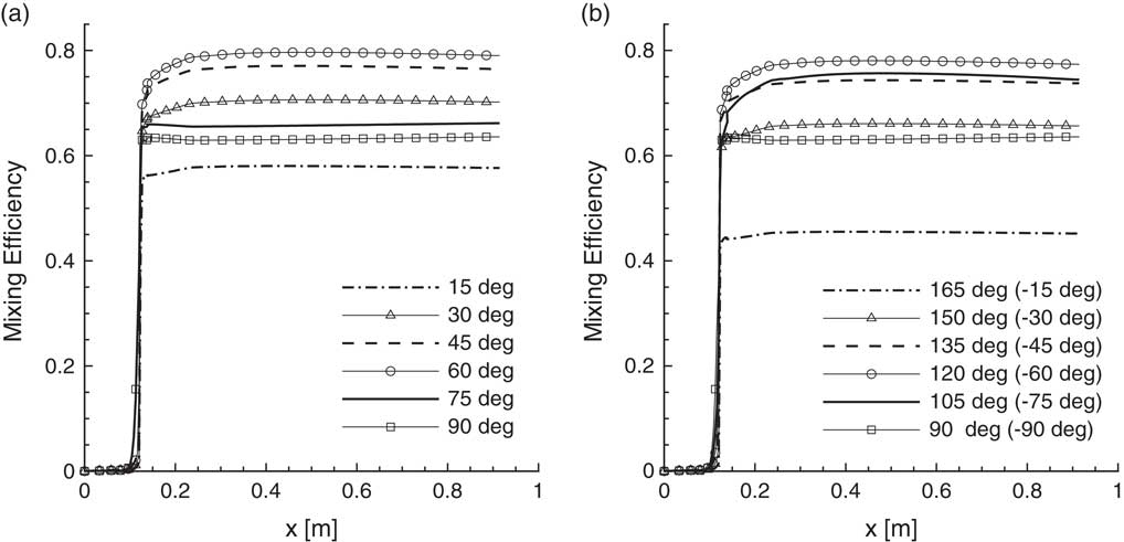
Figure 17 Mixing efficiency for different fuel injection angles. (a) In flow direction and (b) against flow direction.
In the second case, fuel is injected in the upstream direction with different angles. The mixing efficiencies for this case are shown in Fig. 17(b). Likewise, increasing the fuel injection angle up to 60° against the flow direction increases the efficiency of the fuel–air mixing. However, comparing the mixing efficiencies for these two cases shows that injections in the flow direction result in a better performance. This may be due to the fact that injecting the fuel against the flow direction causes a deflection in the high-velocity core flow and prevents the flow from entering the cavity region. Therefore, the recirculation in the cavity region becomes less efficient.
The mixing efficiency is strongly influenced by the secondary flow inside the cavity. Hence, it is important to get insight into how effectively the cavity produces a secondary flow. Figure 18 shows the velocity vectors and streamlines generated over the cavity. In the cavity, the generation of backward flow can be clearly seen. Moreover, streamlines deflect into the cavity region, and just behind the front wall of the cavity, the circulation is developed. This circulation region has a great effect on the mixing efficiency of the chemical reactions.
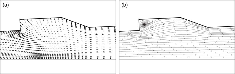
Figure 18 Flow in the cavity region. (a) Velocity vectors and (b) streamlines.
6.0 Conclusion
A CFD code is developed to analyse the flow in a cavity-based scramjet combustor that improves the flameholding properties and mixing efficiency. Ethylene is used as a fuel in the combustion process. The three-dimensional coupled Navier–Stokes and finite rate chemical reaction equations are solved using the JFNK method. The turbulent eddy viscosity is evaluated using the Spalart–Allmaras model. The JFNK method provides a matrix-free solution process, that is, the Jacobian matrix is not explicitly formed or stored. This may be a big advantage in the analyses of scramjet combustor. In the flow solver, convective fluxes are split by Steger–Warming, van Leer and AUSM methods. Results show that although the solutions obtained from these methods are very similar, van Leer and AUSM flux splitting methods are computationally more efficient than the Steger–Warming method. Moreover, the performance of first- and second-order schemes are compared. As expected, first-order schemes are computationally more efficient. The number of iterations and the CPU times are less in first-order schemes, whereas second-order schemes present more details about the flow field. In order to prevent the oscillations in solutions of high-gradient regions, flux limiters are implemented. The performances of different flux limiters are compared for the convergence characteristics of the JFNK method. In terms of computational efficiency, the van Albada limiter shows a better performance. The forcing term strongly influences the computational efficiency of the JFNK method in the flow analyses of scramjet combustor. In general, the higher values of the forcing term reduce the CPU times. In addition, the effects of fuel injection direction and angle on the mixing efficiency are studied. For the analysed cavity configuration, the simulations show that the injection in the flow direction is generally more efficient than the reverse injection. Also, the fuel injection with an angle of 60° gives the best mixing efficiency.
As a future research direction, the convergence performance of the JFNK method can be further improved by preconditioning methods, although they may require forming an approximate Jacobian matrix. In scramjet combustors, turbulence–chemistry interactions can be analysed using different eddy viscosity models and the PDF and the flamelet methods. In the present study, the steady-state flow assumption is imposed. In order to reduce the computational cost, a symmetry boundary condition is imposed at the half plane and the equations are solved in half of the domain. However, unsteady behaviours may be important, especially in cavity recessed scramjet combustors. In unsteady simulations, it is not appropriate to impose the symmetry condition; forcing the symmetry boundary condition may lead to unphysical results. Hence, the entire domain should be solved in unsteady flow analyses. However, this may increase the computational cost significantly. Parallel processing may be needed to reduce the computational time.
Acknowledegment
This research is supported by The Scientific and Technological Research Council of Turkey (TÜBİTAK).


