


NOMENCLATURE
- α
-
level of significance
- β
-
regression coefficient
- C
-
constant
- CR
-
cruise
- FEA
-
Finite Element Analysis
- FEM
-
finite Element Model
- H
-
height (TH and SS parameters)
- HPT
-
high-Pressure Turbine
- HTCs
-
heat Transfer Coefficients
- MDO
-
multi-Disciplinary Optimisation
- n
-
sample size
- PMDO
-
preliminary MDO
- PTO
-
potential To Oversimplify
- SFC
-
Specific Fuel Consumption
- SS
-
shroud Segment
- TO
-
take-Off
- TH
-
turbine housing
- R
-
radius (TH and SS parameters)
- R2
-
coefficient o determination
- W
-
width (TH and SS parameters)
1.0 INTRODUCTION
The gas turbine industry has evolved over the past two decades, characterised by an increase in computer performance and advanced analytical tools. These tools reduced drastically the time required to design a gas turbine. Therefore, in the search for an optimal solution for better engine performances, the number of design iterations increased with an acceptable overall design time. To reach an optimal design process, the complex task of gas turbine design was divided into multiple sub-tasks called disciplines. Then, a trade-off between the disciplines’ requirements was made. This methodology can be referred to as Multi-Disciplinary Optimisation (MDO). The gas turbine design was also divided in two phases: the preliminary phase and the detail design phase. At the detail design phase, efficient interactions between each discipline tool are crucial and it is extremely challenging to make significant changes to the design. To overcome this difficulty, the use of MDO at the preliminary design phase (Preliminary MDO or PMDO) allows making more design iterations where there is more freedom to make modificationsReference Brophy, Mah and Turcotte (1 , Reference Panchenko, Patel, Moustapha, Dowhan, Mah and Hall 2) . PMDO should shorten time for the preliminary design and improve the quality of the results. To implement PMDO, a project with Pratt & Whitney Canada was undertaken to create a set of preliminary design tools focusing on turbine components i.e. rotor, Turbine Housing (TH) and Shroud Segment (SS). Implementation of PMDO generally includes four steps: parameterisation of geometric and performance parameters, development or improvement of correlations, integration of disciplines and components and finally optimisation. The present work focuses on the first two steps with also some integration.
Two key characteristics in an optimum TH and SS design are the calculation of the tip clearance and the SS cooling flow in the High-Pressure Turbines (HPT). The tip clearance has to be selected to achieve the desired turbine efficiency of both rotating and static structures durabilityReference Lattime and Steinetz (3) . A typical increase of 1% in tip clearance/span can result in a drop of 1% in high turbine efficiency, where tip clearance that is 1% of blade span is about 0.2 to 1mm. In addition, the radial movement of rotating and static components is about one hundredth to one tenth of a millimetre. On the other hand, the tip clearance has to be large enough to avoid rubs that reduce the life of rotating and static componentsReference Hennecke (4) . In the evolution of static component geometry, double wall static structures were widely adopted for tip clearance controlReference Lattime and Steinetz (3) . In double wall static structures, the inner wall is the SS facing the main gas path, and the outer wall is the TH. Regarding the SS cooling flow, historically turbine inlet temperature has increased over material limits to achieve better engine performance. The cooling flow used to maintain the SSs below the material limit is usually ducted from compressor sections. Since the Specific Fuel Consumption (SFC) increases with the amount of cooling flow used, SS cooling is a balance between durability and SFC. In order to address this problem, many SS designs were developed to find the best arrangement of impingement, film and convective cooling (5) .
In order to perform the preliminary design and optimisation of THs and SSs with optimal tip clearance and cooling flow, parametric models, geometry and cooling flow correlations were created towards a new design process. The new geometry and cooling correlations minimised the number of parameters used in the design to reduce the turn-around time of the new design process. To explain in more detail what is required to perform the preliminary design and optimisation of TH and SSs, a proposed design process will be presented in Section 2. The focus of this article is on the parameterisation and the development of new correlations that will be presented in Sections 3 to 5. Section 3 covers the creation of the parametric models, while Sections 4 and 5 cover the geometry and the cooling flow correlations.
2.0 PROPOSED DESIGN PROCESS
The proposed design process for gas THs and SSs is presented in Fig. 1. In order to develop a new design process, a centralised data structure is necessary for the integration of the shape definition, analysis, and optimisation modules. At each step of the design, the data is stored in the data structure and the engine parameters are modified through the design. The design process requires a static structure shape definition module which consists in a CAD system and a user interface. The CAD system is a container for the parametric models which is the heart of the design process. In other words, the design process cannot be automated without the parametric models. On the other hand, the user interface is used to modify the parametric models before the initial geometry is analysed. The design process also requires several analysis modules and an optimisation module. Regarding the analysis modules, the design process requires a tip clearance, a cooling flow, and a containment module (i.e. analysis for the containment of failed turbine blades) since those are the three types of analysis performed at the preliminary design phase. In addition, the tip clearance module requires an air system and a thermal module. Finally, the new design process requires an optimisation module because a trade-off between optimal tip clearance, cooling flow and containment has to be made to obtain a balanced design.
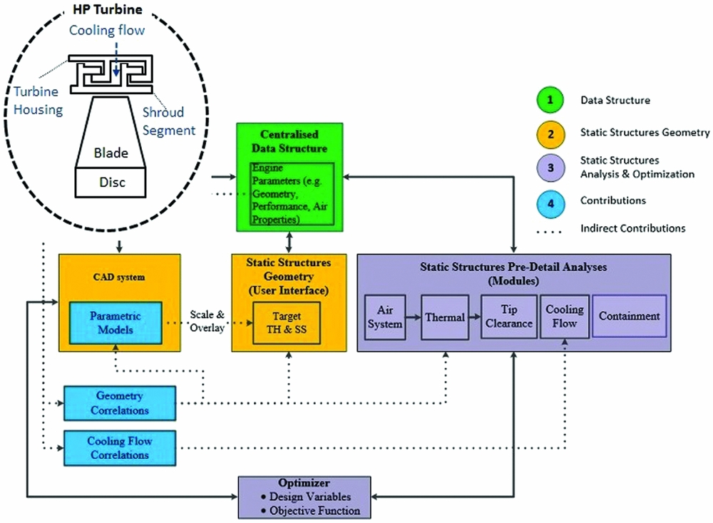
Figure 1. New design process for high-pressure turbine housing and shroud segments.
The novelty and objectives of this work are to develop TH and SS (i.e. the static components above the blade in the HP turbine) parametric models and new geometry and cooling correlations for the shape definition and cooling modules of the static structures. The geometry correlations will also reduce time in the pre-detail analyses.
3.0 PARAMETRIC MODELS
THs and SSs have to be designed with optimal tip clearance, cooling flow, and containment. In order to design TH and SS for optimal tip clearance, the current design process for tip clearance predictions uses a simplified geometry. On the other hand, for optimal cooling flow and containment, only a few engine parameters are used. As a result, the current design process for the tip clearance prediction was used as a starting point to create the TH and SS parametric models.
The current design process for tip clearance predictions is presented in Fig. 2. It consists of a simplified geometry (i.e. rotating and static components) that is drawn on a pre-detail cross-section and the original Tip Clearance Calculator (TCC) that will be replaced by the tip clearance module of the new design process. The dimensions of the geometry are measured and copied into a spreadsheet. Then, the spreadsheet has macros that convert the geometry to create a finite element model. The spreadsheet is also responsible for calculating Heat Transfer Coefficients (HTCs). The geometry and HTCs are transferred to Finite Element Analysis (FEA) software where the transient thermal displacement of the static and rotating components are computed. Finally, the tip clearance is calculated from thermal and centrifugal displacements
Figure 2. Current design process for tip clearance prediction.
In order to show what basis was used in the creation of the parametric models, an example of a simplified TH and SS drawn on pre-detail geometry is presented in Fig. 3. The TH and SS consist of rectangles where fillets, chamfers and non-constant thickness from the pre-detail geometry are ignored. In addition, in the current design process, the radial and axial locations (R1, R2 to Rx and A1, A2 to Ay; {x, y} the number of radial and axial locations) of each line is measured and entered to create a model in a spreadsheet. In the creation of the parametric models, three parameterisation approaches were studied to find the perfect balance between flexibility and complexity i.e. the number of engine configurations a baseline parametric model can reproduce and the engineering effort integrating the parametric models with the analysis modules in the new design process. The parametric models in the three approaches were created using the CAD technique because it had to be consistent with rotating components parametric modelsReference Samareh (6 , Reference Ouellet, Garnier, Roy and Moustapha 7) . This section is divided in two sub-sections: (1) the parameterisation approach and (2) the new TH and SS models.
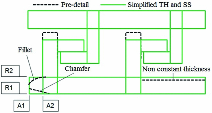
Figure 3. Cross section overlay.
3.1 Parameterisation approach
The skeleton approach consists of a skeleton and an outer shapeReference Mesbah, Seifert, Chatelois, Garnier and Moustapha (8) . The skeleton is represented by the dashed lines and the outer shape is represented by the continuous lines shown in Fig. 4. At least one horizontal and one vertical line of the skeleton must be fixed with a radial and a horizontal parameter. The rest of the skeleton is fixed by a stack-up from the fixed lines of the skeleton. The outer shape is the thickness around each line of the skeleton. A new parameter is required to control the thickness around each line of the skeleton. This approach was useful to study a large quantity of different TH and SS configurations and to simplify them. In the research for a parameterisation approach with higher flexibility i.e. more engine configurations that a baseline parametric model can reproduce, the modular approach was created.
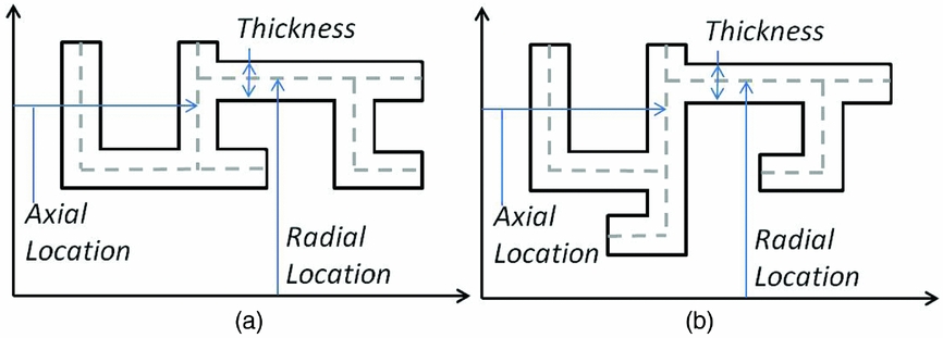
Figure 4 Skeleton approach. (a) Baseline 1, (b) Baseline 2.
The modular approach was developed to address the limited flexibility of the skeleton approach. This approach is defined by components (i.e. groove, bulk of the housing, hooks) that are fixed by their local axis system, represented by a cross, as shown in Fig. 5. Each closed shape can be deactivated. The baseline in Fig. 4 can be reproduced with the modular approach. As a result, the modular approach is limited in flexibility only by the components it has.
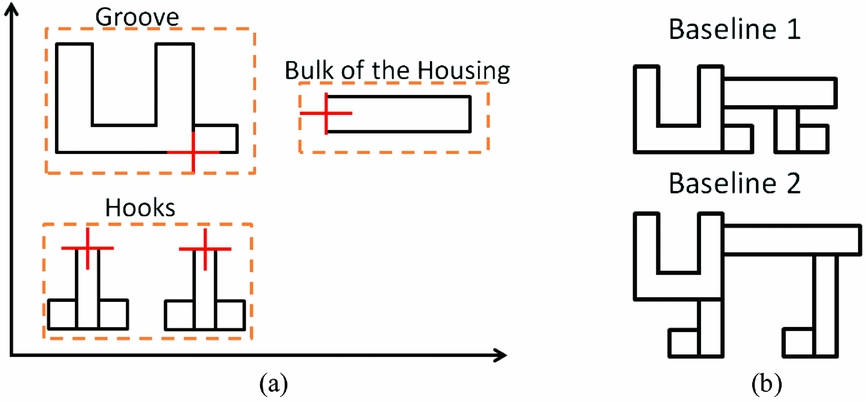
Figure 5. Modular approach. (a) Baseline, (b) Reproduced skeleton baselines.
The downside of the modular approach is also its high flexibility. The parametric models are limited by the complexity in defining the boundary conditions of the finite element model. That is the difficulty in automating the communication with the stator thermal calculator. The thermal boundary conditions automated calculation consists in using the appropriate correlation depending on the surface's topography and the air system distribution. It is thus mandatory to have a limited number of possible configurations to automate the linkage between each surface and the appropriate correlation. This is to allow an inexperienced user to perform a tip clearance study. In order to have predefined boundary conditions, the location of the components relative to one another must be known. For example, if the segment baffle is deactivated or the left hook is at the left of the groove, the boundary conditions will be different. Those differences are depicted in Fig. 6. As a result, the modular approach adds complexity in the development of a fully automated thermal calculator. In order to limit complexity, the fixed modular approach was created.
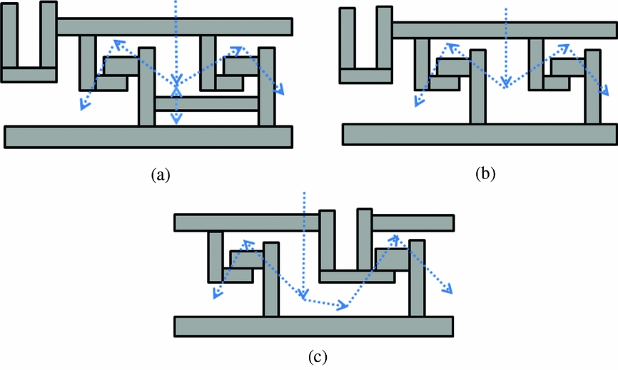
Figure 6 Boundary conditions comparison. (a) with baffle, (b) Deactivated baffle, (c) Left hook moved.
The fixed modular approach is the final approach. It is similar to the modular approach because there are components that can be moved independently from one another. The flexibility of the fixed modular approach is limited such that a stack-up assembles the components together. Then, each baseline configuration is similar to a baseline of the skeleton approach except that the flexibility is increased. For example, the shape of baseline 2 presented in Figs 7 and 5 are the same. The robustness i.e. the number of parameter variations where the integrity of the initial shape is maintained, brought by the independent components of the fixed modular approach allows the creation of a similar shape with a different hook orientation as shown in Figs 7(a) and (b). In addition, the fixed modular approach is faster in creating a new baseline since it is component based. A new baseline with the skeleton approach would require being created from scratch. In addition, in the fixed modular approach, the parameters can be easily chosen such that they are similar to the dimensions of detail-design TH and SSs. Finally, this approach is manageable in terms of defining a set of boundary conditions for each baseline configuration. This approach was used to create the new TH and SS models.
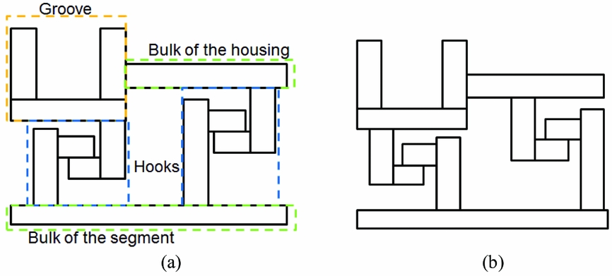
Figure 7. Fixed modular approach. (a) Baseline 2, (b) Baseline 2, hooks flipped.
3.2 New turbine housing and shroud segment models
The new TH and SS models consist of 11 components as presented in Fig. 8. The bulk of the housing (1), the bulk of the segment (2) and the housing and segment hooks (4 to 7) are already available in the current design process. The new components are the optional housing groove (3), the optional segment housing and segment baffles (8 and 9) and the optional rails (10 and 11). In addition, the orientation of the hooks can be modified and the housing groove can be located at the Leading Edge (LE), the centre or the Trailing Edge (TE) of the turbine stage, for the baseline parametric models that include a groove. With the new components and orientable hooks, an increase of 56% in flexibility was observed for the baseline parametric models. An increase in flexibility results in the same increase in geometry accuracy for P&WC engine models. Although an increase in geometry accuracy should result in more accurate tip clearance, cooling flow and containment predictions, the proposed design process has to be completed before an increase in predictions accuracy can be computed. Finally, a user interface was developed and integrated into the new design system to modify the parametric models. The shape of two P&WC TH and SS was reproduced with the user interface and the existing design system to compare the time required for shape definition. Then, the parametric models and the user interface resulted in time saving of 50%. The geometry correlations also contributed to time-saving with the parametric models due to the reduced number of geometric parameters.
Figure 8. New turbine housing and shroud segment models.
Before the geometry correlations were created, TH and SS parametric models had 50 parameters. The main geometry parameters are presented in Fig. 9. Those parameters must be fixed first in shape definition. Some of the secondary geometry parameters are presented in Fig. 10. The parameters W3 to W6, H1 and H2 were renamed and replaced by constants in the geometry correlations section (section 4.0). The remaining parameters are not presented here. They consist of the height and width of the rectangles.
Figure 9. Main turbine housing and shroud segment parameters.
Figure 10. Secondary turbine housing and shroud segment parameters.
4.0 GEOMETRY CORRELATIONS
Parametric models for TH and SSs were created for the new design process. Since the new design process was developed for PMDO, the parametric models have too many parameters. It was previously mentioned that the flexibility of the parametric models was limited using the fixed modular approach by restraining the location of the components (i.e. groove, hooks, etc.). Nevertheless, the flexibility was not limited by creating relations among the geometric parameters. In this section, the second objective of this research consists of reducing the number of geometric parameters with geometry correlations that were developed in three steps: (1) sensitivity analysis, (2) constants and correlations and (3) outlier geometry.
4.1 Sensitivity analysis
The sensitivity analysis consists in verifying that the parametric formulation is not oversimplified. Since many geometric parameters are important in tip clearance, cooling flow and containment predictions, the accuracy of the predictions can be reduced if those parameters are removed. However, the correlations with cooling flow and containment were not computed. Instead, only the correlations with tip clearance were calculated due to the resources available. Since tip clearance is a function of the displacement of the rotating and static components, the thermal displacement of the static components was used to calculate the correlation of the geometric parameters with tip clearance. In order to compare the parameters correlated with the thermal displacement and estimate their potential to oversimplify (PTO) the parametric formulation, a trade-off was made between the sample size n, the level of significance α and the strength of the relation R2. A single value of α should be used in the analysis. However, a higher α means there is a higher probability making an error by concluding there is a correlation( Reference Taeger and Kuhnt 11 , Reference Kreyszig 12 ). For this reason, α = 10% and α = 20% were used and a low PTO was associated with higher α. Second, the sample size varies among the correlations because the number of parameters differs in each parametric model. Since the sample size affects the test of the correlation coefficient and the strength of the relation, a small sample is associated with a lower PTO. Third, the strength of the relation is a good criterion to choose the PTO. However, if R2 is high, n is small and α is high; the PTO is low because R2 on its own does not prove that a parameter is correlated. Finally, the database of thermal displacements was limited in engine models which also explains the small sample size. Then, for additional validation, the correlations were calculated in steady state at two engine operating conditions, Take-off (TO) and Cruise (CR). This methodology was used to isolate the effect of the static component's thermal displacement with the geometry of the SS and TH. The correlations were considered valid, only the observed α value was the same at TO and CR. For example, by using the take-off condition as a reference point, eight parameters were correlated with tip clearance with α = 10% (i.e. R1, R2, R3, R4, R5, W12, H1 and W13). However, for H1 and W13, a higher α = 20% was needed to find a correlation with tip clearance at cruise. Since H1 and W13 are still correlated at TO with α = 20%, they were classified in another category in Table 1.
Table 1 Correlations with static structures thermal displacement
The parameters correlated with the static components thermal displacement are presented in Table 1. It was explained that a trade-off was made between n, α and R2 to assign a PTO to the parameters. The trade-off study was used for the high (H) and the low (L) PTO. However, to assign a medium to high (M-H) and a low to medium (L-M) PTO to R4 and W12, a geometry criterion was used. The PTO for R4 is higher because all the radiuses (i.e. R1, R2, R3, and R5) have a high PTO. On the other hand, for W12, there is a lower PTO because W12 and W13 define the rail widths and W13 has a low PTO. The parameters correlated with the thermal displacement are presented in Fig. 11.
Figure 11. Risk assessment parameters.
4.2 Constants and correlations
In this section, the constants and correlations that were created are presented. The constants are parameters or a group of parameters that don't need to be modified because they show a very small variation among existing engine models. The constants are the radial clearance between the hook and the housing C1, the axial clearance between the hooks C4 and the segment and housing baffle thicknesses C2 and C3. In order to assign an appropriate value for the constants, the average of the samples of existing engine models was calculated. With the four constants presented in Fig. 12, eight parameters were removed from the parametric formulation. Based on industry experience, it was verified that the standardised dimensions and the geometric correlations are acceptable for the design of TH and SS. With the constants and correlations, the reduced parameterisation has 36 parameters compared to the initial parameterisation, which had 50 parameters.
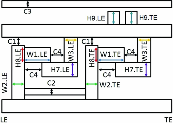
Figure 12. Constants and correlations.
The correlations consist in five hook and one rail correlations. The hook and rail correlations are relations between the LE and the TE dimensions of TH and SS. Those correlations do not use parameters correlated with thermal displacement for tip clearance with medium to high PTO. For the hook and rail correlations, when a strong correlation was observed between the LE and TE dimensions, dependent and independent parameters were created. In order to verify that the correlations were valid, the test of the correlation coefficient was used with α = 5%Reference Taeger and Kuhnt (11) . Then, to properly define dependent and independent parameters, the linear relation between those parameters was established using linear regressionReference Chatterjee and Simonoff (9) . For example, the relation between widths of LE and TE in feet (W1.LE and W1.TE) is presented in Equation (1). The widths in feet for LE and TE are the independent and dependent parameters. Then, W1.LE’ is a function of W1.TE and W1.LE and will replace TE and LE parameters for the shape definition of the static components. Since there is no evidence that W1.TE or W1.LE is more important to design TH and SS, the assumption that the average is more appropriate was made. The average of LE and TE foot width is presented in Equation (2). A new independent parameter W1 was created and W1.LE and W1.TE became dependent parameters. The average was used to create the six parameters presented in Fig. 12. The hook correlations include the feet width W1, the segment and housing leg width W2 and W3 and the segment and housing feet height H7 and H8. The rail correlation is H8.
 $$\begin{equation}
{\rm{W}}1.{\rm L}{\rm{E'}} = \beta 1 + \beta 2*{\rm{W}}1.{\rm{TE}}\\
\end{equation}$$
$$\begin{equation}
{\rm{W}}1.{\rm L}{\rm{E'}} = \beta 1 + \beta 2*{\rm{W}}1.{\rm{TE}}\\
\end{equation}$$
 $$\begin{equation}
{\rm{W}}1 = ({\rm{W}}1.{\rm{LE}} + {\rm{W}}1.{\rm{TE}})/2
\end{equation}$$
$$\begin{equation}
{\rm{W}}1 = ({\rm{W}}1.{\rm{LE}} + {\rm{W}}1.{\rm{TE}})/2
\end{equation}$$
Next, in order to verify that defining LE and TE dimensions as the average of the two was appropriate, the regression error and the error of the average were compared. An example of those errors is presented in Equations (3) and (4). The regression error consists in the difference between W1.LE’ and W1.LE. The error of the average consists in the difference between the average of LE and TE feet width, W1 and W1.LE.
 $$\begin{equation}
{\rm{Regression}}\;{\rm{Error}} = ({\rm{W}}1.{\rm{LE'}} - {\rm{W}}1.{\rm{LE}})/{\rm{W}}1.{\rm{LE}}\\
\end{equation}$$
$$\begin{equation}
{\rm{Regression}}\;{\rm{Error}} = ({\rm{W}}1.{\rm{LE'}} - {\rm{W}}1.{\rm{LE}})/{\rm{W}}1.{\rm{LE}}\\
\end{equation}$$
 $$\begin{equation}
{\rm{Error}}\;{\rm{of}}\;{\rm{the}}\;{\rm{average}} = ({\rm{W}}1 - {\rm{W}}1.{\rm{LE}})/{\rm{W}}1.{\rm{LE}}
\end{equation}$$
$$\begin{equation}
{\rm{Error}}\;{\rm{of}}\;{\rm{the}}\;{\rm{average}} = ({\rm{W}}1 - {\rm{W}}1.{\rm{LE}})/{\rm{W}}1.{\rm{LE}}
\end{equation}$$
The results of the correlations and error comparisons are presented in Table 2. The strength of the relation in the correlations varies from R2 = 71.1% to 100%. With the value of R2, there was enough evidence to suggest that correlations should be created. For the hook correlations, the regression error varies from 4% to 10% and is always bigger than the error of the average that varies from 2% to 9.1%. As a result, defining LE and TE dimensions as the average of the two is more appropriate than using the regression equation. For the rail correlation H9, the error of the average and the regression error are both equal to 0 and R2 = 100%. That is because the LE and TE rails always take the same value. To be consistent, the average was used for H9 as well. Further to that, there is a variable sample size in the hook correlations because outliers were identified and removed. An outlier is an engine with an abnormally large dimension in comparison with the other engines in the sample, thus resulting in a weak correlation. For W3, H7 and H8, weak correlations (i.e. 13.1% for W3, 62.7% for H7 and 57.5% for H8) were observed for larger samples including the outliers. Removing outliers to consider larger R2 is not necessarily a good approach.
Table 2 Hook and rail correlations and error comparison
4.3 Outlier geometry
The geometry for W3 and H8 outliers is presented in Figs 13(a) and (b). The outlier for W3 consists in a wider TH TE hook. Standard THs support only the SSs. A wider TE hook is required to support an additional component with the right portion of the TE hook. On the other hand, the outlier for H8 is represented by an SS with a thicker LE hook. It is thicker because it assembles with non-standard THs. Both W3 and H8 outliers are non-standard designs used in old engine models. Since the correlations were created to facilitate the design of currently used and future engine models, a correlation that does the take into account the geometry of non-standard designs is acceptable.
Figure 13. W3 and H8 outliers.
The outliers identified for H7 are a function of the configuration. Seven TH and SS configurations were identified to create the parametric models. The initial parameterisation for one of the configurations is presented in Fig. 14. In the initial parameterisation, H7.LE was an independent parameter and R4 was not available. In sensitivity analysis, it was found that R4 is correlated with thermal displacement for tip clearance. For this reason, the initial parameterisation was not adequate. The parameterisation was modified to include R4 instead of H7.LE.
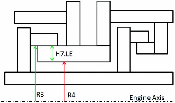
Figure 14. H7 outlier.
5.0 COOLING FLOW CORRELATIONS
Historically the turbine inlet temperature has been increasing over the material limits to achieve better engine performance. With the increase of turbine inlet temperature, the SS is a component at risk of not meeting the minimum life required without cooling. Since the amount of cooling air ducted from compressor sections directly affects the SFC, SS cooling is a trade-off between life and SFC. In this section, the third objective will be addressed i.e. reduce the number of engine parameters used to predict the shroud-segment cooling flow, in the current design process, with correlations. The correlation study on shroud-segment cooling flow was divided in three steps: (1) reviewing the current design process, (2) the creation of a simplified prediction model and (3) the creation of a faster SS selection process.
5.1 Current design process for cooling flow prediction
The current design process for cooling flow prediction is presented in Fig. 15. In order to predict the total segment cooling flow, the cooling flow prediction tool (CFPT) requires:
-
(1) The engine parameters of the new SS (i.e. geometry, performance and air properties);
-
(2) The cooling effectiveness of a new SS;
-
(3) The cooling efficiency of a reference SS.
Figure 15. Current design process for cooling flow prediction.
The cooling effectiveness is necessary to adjust the predicted cooling flow to the maximum metal temperature of the new SS. Finally, to use the appropriate cooling efficiency, the reference and the new SSs must have the same cooling arrangement.
The current SS selection process consists of steps 1 to 4 in Table 3. In step 1, the cooling arrangements are compared and only reference SS 1 and 2, with the same CA observed on the new SS, are considered for steps 2 and 3. In step 2, the difference between the engine parameters of the new and the reference SSs is computed. For example, in Table 3, the difference between the new and reference SS 2 (3-2) is smaller than the difference between the new and reference SS 1 (3-1). The difference is computed for the other parameters. Then, the reference SS presenting a smaller difference in more engine parameters is considered more appropriate. In Table 3, reference SS 2 presents a smaller difference in geometry and air property but not in performance. As a result, in steps 3 and 4, η2 is used to predict the cooling flow of the new SS. It must be mentioned that, in this example, only three parameters are compared. In the current design process, there are 19 engine parameters. In addition, some parameters are more important in the selection of the reference SS. As a result, care must be taken in the choice of a reference. In order to improve time in the current design process, a simplified prediction model and a faster SS selection process were created.
Table 3 Current shroud segment selection process
5.2 Creation of a simplified prediction model
The creation of a new simplified prediction model was conducted in four steps:
-
(1) Compute the correlations with cooling flow. The correlations with cooling flow are essential to narrow down the number of parameters selected to create a regression model.
-
(2) Create a regression model using the best subset, a standard model selection technique.
-
(3) Manually create a regression model function of hot gas and cooling air temperature.
-
(4) Assess the accuracy of the simplified prediction model.
5.2.1 Correlations with cooling flow
In the first step, the correlations between the engine parameters and cooling flow were computed. The results for seven engine parameters are presented in Table 4. Parameters 1 to 5 are correlated with cooling flow. The average gas temperature in the turbine stage, Tgas,avg, shows the strongest correlation with cooling flow with R2 = 88.5%. The four other parameters are highly to averagely correlated with R2 = 84.8% to R2 = 40.1%. Those parameters are: the cooling effectiveness ε or dimensionless metal temperature of the hot surface, the 3D effect, the heat transfer coefficient of the hot surface (HTCgas) and the gas path length. In order to assess the validity of the correlations, the test of the correlation coefficient was used with α ≤ 10%. When a correlation was validated, the corresponding parameter was used to create a regression equation. The correlation for parameters 1 to 4 was validated with α = 5% and parameter 5 with α = 10%. The correlations for the other parameters presenting lower R2 and α ˃ 10 were not validated and hence disregarded.
Table 4 Correlations with cooling flow
Further to that, the new prediction model should include at least cooling-air and hot-gas temperatures. As a matter of fact, in a heat transfer problem, when a solid has a surface exposed to cold air and another surface exposed to hot air, cold and hot air temperatures are required to calculate the temperature of the hot surface. However, the sixth parameter, Tcool,source, or cooling air temperature, is not correlated with cooling flow because R2 = 1.4% and α = 76.1%. Then, to include the cooling air temperature in a regression model, it was verified whether Tcool,source is correlated when combined with other parameters or not. Since Tgas,avg -Tcool,source is highly correlated with R2 = 94.5% and α = 5%, there was hope to create a valid regression model including both hot gas and cooling air temperatures. Parameters 1 to 6 were used to create several regression models that are presented in the next section.
5.2.2 Regression analysis with model selection
The second step consists in the creation of linear regression equations similar to Equation (5). The regression equations include a combination of the six engine parameters mentioned earlier. The standard procedure used to create those equations is the model selection technique called best subset. When the best subset is used, a set of equations also called models is automatically created. Then, one equation is selected to be studied further, based on the R2 a and Cp criterionsReference Chatterjee and Simonoff (10) . When the selected equation does not pass the test of the regression coefficients, another equation is selected until the test is passed.
 $$\begin{equation}
{\rm{Total}}\;{\rm{Segment}}\;{\rm{Cooling}}\;{\rm{Flow}} = {\rm{b}}1 + {\rm{b}}2*{\rm{p}}1 + \ldots + {\rm{b}}7*{\rm{p}}6.
\end{equation}$$
$$\begin{equation}
{\rm{Total}}\;{\rm{Segment}}\;{\rm{Cooling}}\;{\rm{Flow}} = {\rm{b}}1 + {\rm{b}}2*{\rm{p}}1 + \ldots + {\rm{b}}7*{\rm{p}}6.
\end{equation}$$
The best subset was used to create the regression equations A1 to A5 and B1 to B6 that include a combination of the parameters marked with an X in Table 5. In order to be consistent with the test of the correlation coefficient, α = 5% was used for the validation of equations A1 to A5 and α = 10% for equations B1 to B6. What was not mentioned is that the models B1 to B6 were created after the models A1 to A5 were discarded with the test of the regression coefficients. Then, also based on the test of the regression coefficients, the only valid model was B6. However, this model did not meet the research hypothesis that a model should include at least hot-gas and cooling-air temperatures (Tgas,avg and Tcool,source). With a larger sample, the best subset should be more efficient to create a valid regression model. The efficiency estimating all the regression coefficients increases with the degrees of freedom (n – p – 1) where n is the sample size and p the number of predictors. Since the best subset strategy was used with six engine parameters as predictors and a sample size of 8, there is only one degree of freedom, consequently, a small efficiency. Since the best subset failed to create a valid model, additional models were manually created to include only hot gas and cooling air temperatures.
Table 5 Prediction models with the best subset (n = 8; α = 5 and 10%)
5.2.3 Regression analysis with hot gas and cooling air temperatures
For the third and last step of the creation of a new prediction model, two models C1 and C2 were created. Those models are presented in Table 6. First, model C1 was created to include Tgas,avg and Tcool,source. Then, to be more consistent with the current design process, another parameter Tgas,peak was introduced to create the second model C2. The parameter Tgas,peak is the temperature surrounding the hot surface and is also a function of Tgas,avg and the 3D effect, two engine parameters correlated with cooling flow. This can be observed in Fig. 16. The two models were validated with α < 10%. In addition, the strength of the two models is similar with R2 = 96.0% and 95.2%. Since C2 is more consistent with the current design process and C1 is not a much better model based on the value of R2, C2 was selected for the quick cooling flow predictions and the SS selection process.
Table 6 Prediction models with hot gas and cooling air temperatures (n = 8)
Figure 16. Parameters correlated with cooling flow.
5.2.4 Accuracy of the new prediction model
In this section, it will also be determined if C2 can be used as a quick prediction tool by comparing the overprediction and the residuals of the model with the error of the current design process. The results presented in this section do not follow a standard statistical approach. Nevertheless, the results could be used as a basis in future research. The new prediction model is presented in Fig. 17. The predicted and reference cooling flow are represented by a plane and dots. A total of eight references were used to create this model. The predicted cooling flow is a function of the independent variables, Tgas,peak and Tcool,source that were converted in %s. The minimum Tcool,source and the maximum Tgas,peak were defined as 0% and 100%, respectively. To observe the over-prediction and the residuals of the model, a cut at Tcool,source = 1.5% was made. This cut represents the predicted and reference cooling flow as a function of Tgas,peak and a constant Tcool,source.
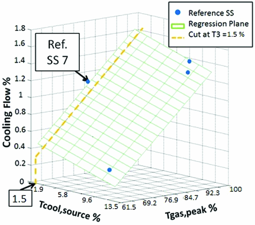
Figure 17. New prediction model C2.
The predicted cooling flow as function of Tgas,peak for a constant Tcool,source = 1.5% is presented in Fig. 18. The predicted cooling flow is represented by a straight line and a 90% PI is represented by dotted lines. A PI of 90% was used to be consistent with the test of the regression coefficients where α = 10% was usedReference Taeger and Kuhnt 11 –Reference Lesik 13 . The reference cooling flow of SS 7 is represented by a dot. In order to assess the accuracy of the new prediction model, the over-prediction (1) and the absolute residual (2) were observed. The over-prediction is the difference between the PI upper limit and the reference flow. The PI upper limit was used because, in SS cooling, it is better to over-predict the cooling flow and reduce it later, at the detail design phase, if possible. On the other hand, the absolute value of the residual is observed because the sum of the residuals of a regression model is usually zero. Further to that, a standard approach to assess the accuracy of a regression model presents the predicted cooling flow and the margin of error (3). However, the accuracy has to be compared to the error of the current design process (4). The error of the current design process is the difference between the reference flow and the predicted flow using the current design process, represented by a circle. As a result, the over-prediction, the absolute residual and the error of the current design process have a common comparison point, the distance from the reference flow. Finally, in Fig. 18, the predicted cooling flow using the current design process was not computed; it is only an example to explain the error of the current design process. The accuracy of model C2 was assessed and compared to the current design process in five test cases that are presented later on.
Figure 18. Predicted cooling flow as function of Tgas,peak for a constant Tcool,source = 1.5%.
The five test cases A, B, C, D and E used to compare the accuracy are presented in Table 7. In the five test cases, the absolute residual, the overprediction and the error of the current design process, were divided by the reference cooling flow to have a logic comparison point. In case A, the absolute residual is 9% and the over-prediction is 108%. In comparison, the error of the current design process is smaller (0.02%). In all the test cases, the current design process is more accurate than the absolute residual. This proves that, even without a PI (i.e. no margin of error), the current design process is more accurate than model C2. In cases A to D, the current design process is more accurate than the over-prediction. On the other hand, case E shows 21% of error for the current design process and the over-prediction and a larger error or 27% for the absolute residual. A larger residual indicates that the reference flow is closer to PI upper limit. A larger error of 21% shows that the current design process can be improved. Finally, the average error confirms that the current design process is more accurate with 9% compared to the average residual 17% and overprediction 64%. As a result, model C2 cannot be used to replace the current design process. Then, model C2 was used to create a simplified SS selection process.
Table 7 Model C2 VS current design processes
5.3 Simplified shroud segment selection process
The simplified SS selection process is presented in Fig. 19. It is similar to the current SS selection process. First, the reference and new SSs must have the same cooling arrangement. Second, the 2D representation of the new prediction model is used to observe how distant two SSs are from one another in Tcool,source (1), Tgas,peak (2) and predicted cooling flow (3). For example, the horizontal, vertical and diagonal distances between the SSs 7 and 8 are calculated because they have the same cooling arrangement. Those distances are calculated for a second SS with the same cooling arrangement. The hypothesis is that a closer reference SS will provide more accurate results. Then, the reference SS closer to the new SS is used in the predictions. Although this seems a promising approach, the simplified SS selection process does not prove that a closer reference SS provides more accurate cooling flow predictions. A limit around the new SS must be defined. This will be explained in the following three test cases.
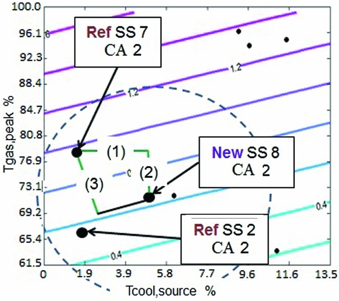
Figure 19. Simplified shroud segment selection process.
The error of the current design process was calculated for three test cases (3 SS) in Table 8 to verify if the new SS selection process (i.e. ∆Tgas,peak, Tcool,source and Predicted cooling flow) can be used to select the most appropriate SS.
Table 8 Shroud segment selection process test case
In the first test case, the reference SSs 7 and 2 were used to predict the cooling flow of SS 8. Reference SS 7 is a better choice because the current design process error is smaller (11% < 21%). However, the simplified SS selection process would suggest that reference SS 2 is a better choice because it is closer in Tcool,source (3.2 < 3.5), Tgas,peak (5.7 < 6.5) and predicted cooling flow (0.107 < 0.307).
In the second test case, the reference SSs 7 and 8 were used to predict the cooling flow of SS 2. Reference SS 7 is a better choice with an error of 14%. However, the simplified SS selection process does not prove that either of reference SS 7 and 8 are better. As a matter of fact, reference SS 7 is closer in Tcool,source (0.3 < 3.2) but farther in Tgas,peak (12.1 ˃ 5.7) and predicted cooling flow (0.414 < 0.107). Then, there may be one parameter that is more important to determine which reference is more appropriate.
In the third test case, the reference SSs 8 and 7 were used to predict the cooling flow of SS 9. Reference SS 8 is a better choice with an error of 0.031%. The simplified SS selection process is in agreement with this result since reference SS 8 is closer in Tcool,source, Tgas,peak and predicted cooling flow.
The new SS selection process is inconclusive in terms of selecting the most appropriate reference SS because only one test validated the hypothesis. It is possible that when the reference SS is close enough, the new SS selection process is a good alternative to the current SS selection process. To verify this, the new SS selection process should be revisited with a distance limit. For example, with values slightly bigger than reference 8 in test case 3, a limit of ±1.5% in Tcool,source and Tgas,peak and a limit of ±0.100% in predicted cooling flow should be used. Since the reference and the new SSs must have the same cooling arrangement, additional reference SSs must be created to assess the efficiency of the proposed limits or to propose new limits.
6. CONCLUSION AND RECOMMENDATION
TH and SSs parametric models and a user interface were created for the shape definition module of the proposed design process. The parametric models and the user interface resulted in a time saving of 50% and an increase in accuracy of 56% compared to the existing design system. Finally, the parametric models were created to design cooled TH and SS. Additional work is necessary to verify if they are adequate to design uncooled TH and SS.
New geometry correlations were created to minimise the number of parameters used to design TH and SS. With the four constants and the six correlations, the number of parameters was reduced from 50 to 36. As a result, the geometry correlations also resulted in time-saving compared to the existing design system. The correlations with thermal displacement for tip clearance were also computed to assess the risk of removing too many parameters from the parametric formulation. Future studies are needed to assess the risk of over-simplifying the parametric formulation for cooling flow and containment predictions.
Regarding the new cooling flow correlations, a new prediction model was created. Then, the model was used to create a simplified SS selection process that could contribute having quicker cooling flow predictions if additional work was done to find temperature range.
Based on the ongoing and future work for the integration and the optimisation as well as industry experience on previous preliminary design, it was estimated that the parametric models and the new correlations contributed about 30% of the total work needed to develop a total PMDO for SS and TH. In order to obtain the new design process, the remaining analysis modules and optimiser capable of finding a balanced design (i.e. optimal tip clearance, cooling flow and containment thickness) will be created.
ACKNOWLEDGEMENTS
The authors would like to acknowledge ASME for permission to publish the ASME paper N ° GT2016-56686.
This work was funded by Pratt and Whitney Canada (P&WC) and the National Sciences and Engineering Research Council of Canada (NSERC). The authors would like to thank them for their contribution to this project.
SUPPLEMENTARY MATERIAL
To view supplementary material for this article, please visit https://doi.org/10.1017/aer.2017.135


