NOMENCLATURE
- c
-
blade choord
- Ak, Bk, Ck, Dk
-
discrete time model matrices
- AC k, BC k, CC k, DC k
-
periodic controller matrices
- CL, CD, CM
-
lift, drag and moment coefficients
- CnM 2
-
sectional normal force coefficient
- E{., .}
-
variance matrix
- E[.]
-
expected value
- F
-
tip-loss correction factor
- Fz
-
blade root shear force
- FZ
-
hub vertical force
- J
-
performance index
- Kk
-
feedback proportional gain
- MX, MY
-
hub moment along x and y axis
- N
-
discrete controller period
- Ok
-
observability matrix
- p
-
pitch bearing position
- Q i k , R ij k
-
QR factorisation matrices of U k, s and Y k, s , (i, j) = {1, 2}
- R
-
blade radius
- U k, s , Y k, s
-
input and output Hankel matrices
- Uk , Σ k , Vk
-
singular value decomposition matrices of R 22 k
- TZ
-
rotor thrust
- u
-
system control
- V
-
electric potential
- V ∞
-
free-stream velocity
- w
-
white noise
- Wdist
-
baseline loads shaping filters
- Wn
-
disturbance shaping filters
- Wperf
-
performance weighting function
- x, y
-
system state and output vectors
- z
-
system performance
- α
-
shaft angle
- ϑ p
-
pre-cone angle
- ϑ tw
-
blade twist
- μ
-
advancing ratio
- νβ
-
non-dimensional flap frequency
- νϑ
-
non-dimensional torsional frequency
- νξ
-
non-dimensional lag frequency
- Ω
-
rotor angular velocity
1.0 INTRODUCTION
Helicopters experience severe levels of vibration on the main rotor due to the asymmetrical airflow in forward flight. These vibratory loads are transmitted to the fuselage and degrade the flight comfort, while causing structural components fatigue and wear. Active controls are being extensively investigated by helicopter researchers to reduce the related vibrations. The basic strategy to alleviate such loads is to modify the periodic aerodynamic loads at harmonic frequencies above the 1/rev. The simplest approach is to control the already available swashplate through a suitable harmonic signal computed by the Higher Harmonic Control (HHC) algorithm(Reference Patt, Chandrasekar, Bernstein and Friedmann1), based on a linear quasi-static rotor model response. However, it is now possible to embed actuators into the blades and thus to independently control each blade. This allows to overcome the limitations of using only a swashplate as actuator, such as the need to install otherwise over-dimensioned hydraulic actuators and the impossibility to independently control more than three blades. Different methods of actuation have been studied to carry out Individual Blade Control (IBC)(Reference Wilbur and Wilkie2-Reference Ravichandran, Chopra, Wake and Hein5). In this paper, we assume the availability of actively twisted blades. Piezoelectric actuators are distributed along the blade span, with the control voltage computed to minimise the aerodynamic loads. This solution has been widely investigated in recent years(Reference Pawar and Jung6,Reference Althoff, Patil and Traugott7) , and experimental tests carried out at NASA(Reference Wilbur and Wilkie2) and DLR(Reference Monner, Riemenschneider, Opitz and Schulz8,Reference Riemenschneider and Opitz9) proved its feasibility.
The complex non-linear behaviour of the rotor subsystem in forward flight limits the possibility of achieving satisfactory performance through linearised time invariant controller theories. In particular, the dynamic system periodicity plays an important role, so that more sophisticated solutions can be found by exploiting the periodic control theory. A model following approach to stabilise lag and pitch moments using periodic control has been proposed by Vaghi(Reference Vaghi10). Periodic vibration controllers were also used by Arcara et al(Reference Arcara, Bittanti and Lovera11) and by Bittanti and Cuzzola(Reference Bittanti and Cuzzola12); both these papers consider the baseline loads alleviation by means of IBC as a disturbance rejection problem. Active twist flaps are used by Ulker(Reference Ulker13) to reduce hub loads by a dynamic compensator arising from the periodic H 2 and H ∞ design.
In the present paper, we start from a review of the periodic H 2 design and of the Periodic Output Feedback (POF) technique(Reference Brillante, Morandini and Mantegazza14,Reference Brillante, Morandini and Mantegazza15) to reduce hub loads. After comparing the two solutions and showing that satisfactory results can be achieved by using the static POF approach, we test the robustness of the two controllers. It is shown that, even if a simple design model is used in the design phase of the vibration periodic controllers, satisfactory load reductions are achieved with a more complex numerical model that better approximates the real rotor behaviour. An important aspect of this study is the analysis of the POF controller: its design is very simple and involves fewer parameters than those of the H 2 controller. Another advantage is that all the helicopter flight envelope can be covered with an easy gains scheduling.
The paper is organised as follows. In the Section 2.0, the rotor numerical model and the tools used to simulate the response of both the design and the validation model are described. In the Section 3.0, the blade response of the design model is properly identified, and the procedures to synthesise the periodic H 2 controller and the POF one are explained. Section 4.0 shows the validation model closed-loop results and assesses the controller’s robustness.
2.0 NUMERICAL MODELLING
2.1 Multi-body rotor model
Vibratory forces acting on the hub can be reduced by modifying the periodic aerodynamic loads in the forward flight condition. Blades actively twisted by means of piezoelectric actuators distributed along the blade span are considered here. The original blades of an already available multi-body model of the Bo 105 rotor(Reference Dieterich, Götz, DangVu, Haverdings, Masarati, Pavel, Jump and Massimiliano16) are replaced with actively twisted ones. The active blades use Macro-Fibre Composite (MFC) piezoelectric actuators with inter-digitated electrodes. These actuators exploit the primary piezoelectric direction of polarisation, thus allowing to achieve a high strain rate with low actuation power. They are oriented in such a way that the strain is applied at
 $\pm 45\deg$
to generate maximum torsional authority.
$\pm 45\deg$
to generate maximum torsional authority.
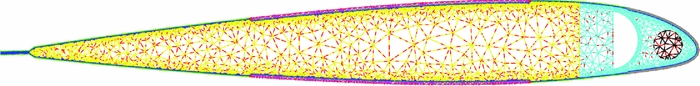
The inertial couplings and structural deformation of the main helicopter rotor are intrinsically non-linear. Therefore, the use of a suitable non-linear model is mandatory. A deformable multi-body model, built with the software MBDyn(Reference Masarati, Morandini and Mantegazza17), is used. The swashplate and the pitch links are represented with rigid bodies, while each blade is modelled using five geometrically exact finite volume non-linear beam elements(Reference Ghiringhelli, Masarati and Mantegazza18). MBDyn is able to handle piezoelectrically actuated beams provided the stiffness, and the piezoelectric coupling matrices of the blade section are known. The beam section stiffness and mass data of the original Bo 105 blades are known. The section properties of the actively twisted blades, on the contrary, have to be computed. An accurate way to compute such properties, still accounting for three-dimensional elastic and piezoelectric constitutive laws, is the semi-analytical approach(Reference Ghiringhelli, Masarati and Mantegazza19-Reference Brillante, Morandini and Mantegazza21). The three-dimensional continuum is decomposed into the one-dimensional domain of the beam model and the two-dimensional domain of the beam section. A finite element discretisation of the beam section, such as that shown in Fig. 1, allows computing, by means of a specialised semi-analytic procedure, the sought generalised beam section stiffness matrix. This semi-analytical formulation was used to optimise the piezoelectric blade section(Reference Ghiringhelli, Masarati, Morandini and Muffo22); the position of the elastic axis and of the centre of mass were constrained during the optimisation to avoid aeroelastic instabilities. Rotor data, together with the first frequencies of the original passive blades and of the optimised piezoelectric blades, are shown in Table 1.

Figure 1. Blade section discretisation.
Table 1 Bo 105 model data with original and piezoelectric blade

Even though MBDyn is a general-purpose multi-body software, it contains some specialised elements for the simulation of helicopter rotors; among them, it provides simple aerodynamic elements, such as the blade element momentum theory and different linear inflow models. Taken together, these elements allow a quick approximation of the system response with a level of accuracy that is deemed suitable to reproduce representative vibratory loads in forward flight, at least for a preliminary design of the controller. The simulations were performed by combining the Blade Element Momentum (BEM) theory with the Drees inflow model(Reference Leishman23). The required data are the lift, drag and moment coefficients of the blade NACA 23012 aerofoil, CL, CD and CM , with respect to the Mach number and to the aerodynamic angle-of-attack. This rotor model will be later referred to as the ‘low-fidelity model’ because it is based on a low-fidelity aerodynamic model. It has been used to design the controllers through several optimisations.
2.2 Free-wake aerodynamic code
A more accurate model is required to validate the controller’s performance. The multi-body deformable structural model is detailed, well tested, and validated. The aerodynamic model, on the other hand, is rather simple and can strongly influence the predicted loads acting on the blades. In particular, linear inflow models are known to under-estimate the harmonic content of the forces. Computational Fluid Dynamics (CFD) is usually used to solve the aerodynamic field of every single blade, while the induced velocity is computed through potential methods, such as the prescribed or free-wake method(Reference Abedi24). However, we strive to avoid computationally intense tasks, such those arising from CFD simulations, because we need to simulate several seconds of flight to validate the controllers. For this reason, we have chosen the so-called hybrid approach(Reference Sheng, Zhao, Rajmohan and Sankar25-Reference Amiraux27), thus treating separately, with different models, the aerodynamic near and far fields of the blade. An improved blade element theory accounting for unsteady effects is used for the near field representation. The rotor wake is approximated by releasing the blade-tip vortex at each time-step; the ensuing free-wake dynamic is integrated in time, with the induced velocity computed according to the Biot-Savart law.
The blade span is divided into strips, with more elements at the blade root and tip; a tip-loss factor is defined as well. The tip-loss correction factor F scales the aerodynamic coefficients of each strip and is computed according to the simplified Prandtl’s formulation(Reference Leishman23,Reference Betz28) . The lift, drag and aerodynamic moment of the strip is computed through the data sheet for the CL, CD and CM coefficients that was used for the MBDyn simulations and scaled by the tip-loss factor F. The effective aerodynamic angle-of-attack, however, is corrected by accounting for unsteady effects; this is achieved by using both the Theodorsen lift deficiency function for the aerofoil motion and the Kussner function, which better represents the interaction between the blades and the tip vortexes, considered as gusts(Reference Bisplinghoff, Ashley and Halfman29,Reference Hansen, Gaunaa and Madsen30) .
After computing the loads of every blade element, the equivalent bound circulation is computed through the Kutta-Jukovsky theorem, and the strength of the tip vortex that is going to be released at a given time-step is set to the 80% of the maximum bound circulation of the blade outer portion(Reference Vermeer31), with a dual-peak model in case of a negative load on the outer portion of the blade tip(Reference Johnson32). An important model parameter is the size of the vortex core. Since we are only using the tip vortex to approximate the rotor wake, reproducing the physical size of the core vortex would over-estimate the blade vortex interaction loads(Reference Amiraux27); thus, we assume that the blade-tip vortex initial diameter is equal to 50% of the blade chord(Reference Johnson33) and that the vortex aging follows Squire’s law(Reference Amiraux27,Reference Leishman, Bhagwat and Ananthan34) . The effects of the near wake are taken into account by the unsteady blade element theory and the tip-loss correction; for this reason, the far wake represented by the tip vortexes is activated after 30° of rotor revolution. The aerodynamic code is written in Matlab.
MBDyn can perform co-simulations by exchanging data with external programs by means of bi-directional socket communications; a Python communication library is available to ease the interfacing effort. Therefore, the Matlab free-wake code is connected to MBDyn through the open-source software MatPy(35), a useful Python interpreter for Matlab. The aeroelastic interface between the structural node of the beams and the aerodynamic strip elements is computed through an energy-conserving moving least-squared algorithm(Reference Quaranta, Masarati and Mantegazza36).
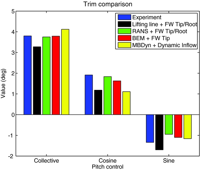
The simulation code has been validated with the experimental data of the Hart II baseline trim condition, a 6° descent flight at μ = 0.15(Reference Sa, Kim, Park, You, Park, Jung and Yu37). Figure 2 compares the experimental collective and cyclic pitch control against those computed with our free-wake code, with the blade element theory combined with the dynamic inflow of MBDyn, and with the two hybrid approaches described by Amiraux(Reference Amiraux38). In the first approach, the lifting line theory is combined with the free-wake geometries of the tip and the root vortexes, while in the second approach a more accurate RANS-based CFD code is used for the near-field aerodynamics of the blade. To better evaluate the BVI prediction and the loads estimation capabilities of the code, the normal force coefficient of the section at 87%R is compared, for one rotor revolution, in Fig. 3. The normal force coefficient predicted by our code is close to that obtained with the lifting line theory with only the free wake of tip vortex; it is also able to predict the position of the BVI. However, both codes overestimate the BVI peaks. The more accurate and computationally demanding RANS model with tip and root vortexes reduces the BVI peaks and better approximates the low-frequency content of the normal-force coefficient. Moreover, the lifting line and BEM methods produce a lower peak in CnM 2 near 115°, while experiment and RANS solver lower peaks are closer to 160°. This phase shift will have an impact on 4/rev loads. Thus, the proposed code is not able to match the more accurate response of the RANS plus tip/root vortexes schemes. However, it reproduces with a much smaller computational cost the overall response of the real system. It will thus be used as a verification model to assess the proposed controller robustness.

Figure 2. Hart II baseline trim condition, 6° descent flight at μ = 0.15.

Figure 3. Normal-force coefficient comparison, 87% R.
3.0 CONTROLLER DESIGN
3.1 Identification of the design model
The design model, based on the low-fidelity aerodynamic theory provided by MBDyn, allows the controller to be tuned with a reasonable computational effort. The effect of the control applied to one blade on the forces on the other blades is almost null due to the very simple aerodynamic model. Therefore, each blade is considered independent, and the IBC controller is designed by considering only a single blade. A periodic state-space model linearised around an equilibrium configuration is required for the periodic control design. The linearised input/output relation between the voltage V applied on the blade and the blade sensors measures is of interest. The blade root shear force Fz and five vertical accelerations at locations uniformly distributed along the blade span are chosen as outputs in order to well represent the blade response for the identification.
Dealing with a helicopter in forward flight, the system is periodic. This has to be taken into account when identifying the model. Classical identification procedures for Linear Time Invariant (LTI) systems cannot be used for periodic systems. Thus, a periodic subspace identification algorithm(Reference Ulker13) is used to find a Linear Discrete-time Periodic (LTP) model of the blade in the form:
 $$\begin{eqnarray}
\mathbf{x}_{k+1} &=&\mathbf{A}_{k}\mathbf{x}_{k}+\mathbf{B}_{k}u_{k},\nonumber \\
\mathbf{y}_{k} & =&\mathbf{C}_{k}\mathbf{x}_{k},
\end{eqnarray}$$
$$\begin{eqnarray}
\mathbf{x}_{k+1} &=&\mathbf{A}_{k}\mathbf{x}_{k}+\mathbf{B}_{k}u_{k},\nonumber \\
\mathbf{y}_{k} & =&\mathbf{C}_{k}\mathbf{x}_{k},
\end{eqnarray}$$
where the system matrices have period N. The input/output time histories signals from the numerical simulations are organised in input/output Hankel matrices U k, s and Y k, s for k = 1. . .N as follows:
 $$\begin{eqnarray}
\mathbf{U}_{k,s} & =\left[\begin{array}{cccc}u_{k} & u_{k+1} & \cdots & u_{k+s-1}\\
u_{N+k} & u_{N+k+1} & \cdots & \vdots \\
\vdots & & \cdots & \vdots \\
u_{(n-1)N+k} & & \cdots &\,\, u_{(n-1)N+k+s-1} \end{array}\right],
\end{eqnarray}$$
$$\begin{eqnarray}
\mathbf{U}_{k,s} & =\left[\begin{array}{cccc}u_{k} & u_{k+1} & \cdots & u_{k+s-1}\\
u_{N+k} & u_{N+k+1} & \cdots & \vdots \\
\vdots & & \cdots & \vdots \\
u_{(n-1)N+k} & & \cdots &\,\, u_{(n-1)N+k+s-1} \end{array}\right],
\end{eqnarray}$$
 $$\begin{eqnarray}
\mathbf{Y}_{k,s} & =\left[\begin{array}{cccc}y_{k} & y_{k+1} & \cdots & y_{k+s-1}\\
y_{N+k} & y_{N+k+1} & \cdots & \vdots \\
\vdots & & \cdots & \vdots \\
y_{(n-1)N+k} & & \cdots &\,\, y_{(n-1)N+k+s-1} \end{array}\right],
\end{eqnarray}$$
$$\begin{eqnarray}
\mathbf{Y}_{k,s} & =\left[\begin{array}{cccc}y_{k} & y_{k+1} & \cdots & y_{k+s-1}\\
y_{N+k} & y_{N+k+1} & \cdots & \vdots \\
\vdots & & \cdots & \vdots \\
y_{(n-1)N+k} & & \cdots &\,\, y_{(n-1)N+k+s-1} \end{array}\right],
\end{eqnarray}$$
where N is the period, n is the total number of simulations and s is the length of each experiment. The Hankel matrices are computed using data from the numerical simulations. Considering the QR factorisation of the compound matrices:
 $$\begin{equation}
\left[\begin{array}{c@{\quad}c}\mathbf{U}_{k,s} & \mathbf{Y}_{k,s}\end{array}\right]=\left[\begin{array}{c@{\quad}c}\mathbf{Q}_{1_{k}} & \mathbf{Q}_{2_{k}}\end{array}\right]\left[\begin{array}{c@{\quad}c}\mathbf{R}_{11_{k}} & \mathbf{R}_{12_{k}}\\
\mathbf{R}_{21_{k}} & \mathbf{R}_{22_{k}} \end{array}\right],
\end{equation}$$
$$\begin{equation}
\left[\begin{array}{c@{\quad}c}\mathbf{U}_{k,s} & \mathbf{Y}_{k,s}\end{array}\right]=\left[\begin{array}{c@{\quad}c}\mathbf{Q}_{1_{k}} & \mathbf{Q}_{2_{k}}\end{array}\right]\left[\begin{array}{c@{\quad}c}\mathbf{R}_{11_{k}} & \mathbf{R}_{12_{k}}\\
\mathbf{R}_{21_{k}} & \mathbf{R}_{22_{k}} \end{array}\right],
\end{equation}$$
the observability matrix O k is given by the row space of matrix R 22 k . It can be computed through the singular value decomposition (SVD):
 $$\begin{equation}
\mathbf{R}_{22_{k}} =\mathbf{U}_{k}\bm{\Sigma }_{k}\mathbf{V}_{k}^{T}
\end{equation}$$
$$\begin{equation}
\mathbf{R}_{22_{k}} =\mathbf{U}_{k}\bm{\Sigma }_{k}\mathbf{V}_{k}^{T}
\end{equation}$$
 $$\begin{equation}
\mathbf{O}_{k} =\tilde{\mathbf{V}}_{k}^{T}.
\end{equation}$$
$$\begin{equation}
\mathbf{O}_{k} =\tilde{\mathbf{V}}_{k}^{T}.
\end{equation}$$
The order of the identified system is chosen according to the magnitude of the singular values of
Σ
k
. Then, the observability matrix is computed as
 $\tilde{\mathbf{V}}_{k}^{T}$
, which contains the first rows and columns of V
T
k
up to the defined system order. Afterward, the matrices A
k
and C
k
can be obtained by exploiting the observability matrix at the instants k + 1 and k
(Reference Ulker13,Reference Verhaegen and Yu39) . The system periodicity is imposed by setting O
N + 1 = O
1.
$\tilde{\mathbf{V}}_{k}^{T}$
, which contains the first rows and columns of V
T
k
up to the defined system order. Afterward, the matrices A
k
and C
k
can be obtained by exploiting the observability matrix at the instants k + 1 and k
(Reference Ulker13,Reference Verhaegen and Yu39) . The system periodicity is imposed by setting O
N + 1 = O
1.
Matrices B k and D k are computed by minimising the squared 2-norm error between the real and the model outputs, yreal and y, respectively:
 $$\begin{equation}
{\it min}\hspace*{-18pt}{{}\atop{_{\mathbf{B}_{k},\mathbf{D}_{k}}}}\hspace*{-4pt}\parallel y_{real}-y\parallel _{2}^{2}.
\end{equation}$$
$$\begin{equation}
{\it min}\hspace*{-18pt}{{}\atop{_{\mathbf{B}_{k},\mathbf{D}_{k}}}}\hspace*{-4pt}\parallel y_{real}-y\parallel _{2}^{2}.
\end{equation}$$
The rotor is trimmed at an advance ratio μ = 0.23 so to reproduce reasonable hub forces, TZ = 20, 010 N, MX = 746 Nm and MY = −85 Nm, with a shaft angle of α = 3° as in Fig. 4. The blade periodic loads and the accelerations for the reference trimmed configuration are saved; they are subsequently subtracted from the excited response signals to linearise the system around the trimmed configuration. The blade are excited with a random voltage with an amplitude of 40 V filtered above 6/rev to limit higher harmonics in the dynamic response. The Bo 105 rotor has a four blades; thus, the most important harmonics for the vibratory hub loads are the 3/rev and the 4/rev; all output signals have been filtered before the identification to consider only these harmonics, hence reducing the size of the state-space model. The controllers should minimise the 4/rev harmonic of the blade root shear force Fz to reduce the hub vertical force and reduce the 3/rev harmonic as well to alleviate the vibratory loads associated to the moments of the blade root loads. Note that for the vertical force and the torque of the hub only the steady and the multiples of the 4/rev harmonics of the blade root force and moment are not filtered by the hub. On the other hand, the multiples of the 4/rev in plane forces and moments of the hub, with respect to the rotor disk, are generated by the multiples of the 3/rev and 5/rev blade loads and moments. The aeroelastic multi-body simulation requires a small integration time-step; the simulations are performed with N = 140 time-steps for every rotor revolution. The direct identification of such signals will lead to the computation of 140 linear systems spanning the period. The system outputs are decimated to N = 28 time-steps per rotor revolution in order to reduce the computational burden of both the identification and the controller design, still approximating the outputs with sufficient accuracy. Hints about the order of the identified system can be found by analysing the singular value magnitudes of the matrix R 22 k at each time-step. The best compromise between data fitting and system order is given by retaining the most important singular values. For example, Fig. 5 shows the singular values computed for the first time-step. Based on the singular values, the chosen linear periodic model of the blade is a 14th-order system for every time-step spanning the period.
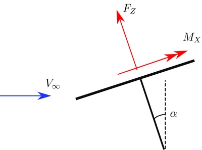
Figure 4. Rotor shaft inclination.
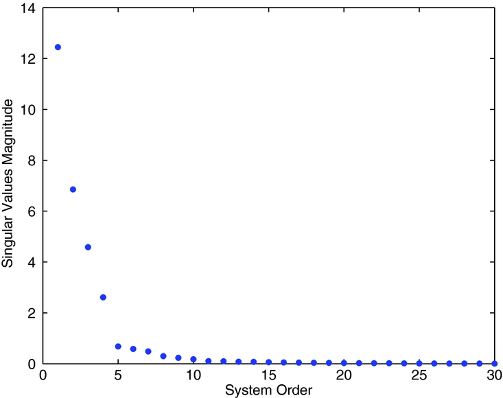
Figure 5. Hankel singular values magnitude of R 22 k .
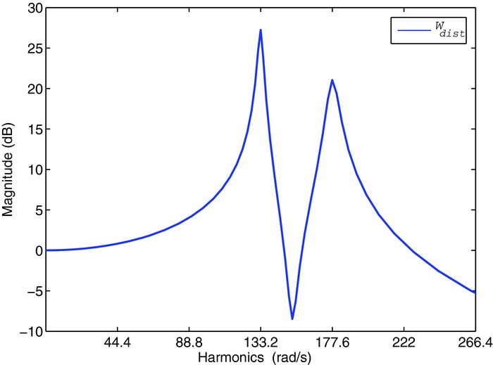
After identifying the linearised blade model, performance specifications and model disturbances have to be introduced in the generalised plant. The block diagram of the complete design model is shown in Fig. 6, where z are the controlled outputs, y are the measures, w are white noise disturbances and u the applied blade voltage. The goal is to minimise the blade root shear force Fz . The shaping filters Wdist models the baseline loads, which are now reintroduced as output disturbances of the system. Figure 7 shows the shaping filter that models the baseline load of the tip blade acceleration; since the measures have been previously filtered, only the 3/rev and the 4/rev harmonics of the baseline signals have to be reproduced. The sensors noise is modelled with white noises having an amplitude of 0.1. The performance of the controller are defined by means of the frequency weighting function Wperf , shown in the block diagram of Fig. 6, to impose the reduction of the blade root load Fz harmonics; it is adjusted in the controller design phase to obtain the best vibration reduction. The generalised plant model is thus described with the following linear periodic model:
 $$\begin{eqnarray}
\mathbf{x}_{k+1} &=&\mathbf{A}_{k}\mathbf{x}_{k}+\mathbf{B}_{1_{k}}\mathbf{w}_{k}+\mathbf{B}_{2_{k}}V_{k},\nonumber \\
\mathbf{z}_{k} &=&\mathbf{C}_{1_{k}}\mathbf{x}_{k}+\mathbf{D}_{11_{k}}\mathbf{w}_{k}+\mathbf{D}_{12_{k}}V_{k},\\
\mathbf{y}_{k} &=&\mathbf{C}_{2_{k}}\mathbf{x}_{k}+\mathbf{D}_{21_{k}}\mathbf{w}_{k}\nonumber
\end{eqnarray}$$
$$\begin{eqnarray}
\mathbf{x}_{k+1} &=&\mathbf{A}_{k}\mathbf{x}_{k}+\mathbf{B}_{1_{k}}\mathbf{w}_{k}+\mathbf{B}_{2_{k}}V_{k},\nonumber \\
\mathbf{z}_{k} &=&\mathbf{C}_{1_{k}}\mathbf{x}_{k}+\mathbf{D}_{11_{k}}\mathbf{w}_{k}+\mathbf{D}_{12_{k}}V_{k},\\
\mathbf{y}_{k} &=&\mathbf{C}_{2_{k}}\mathbf{x}_{k}+\mathbf{D}_{21_{k}}\mathbf{w}_{k}\nonumber
\end{eqnarray}$$
It can be noticed that there is no direct feed-through between the input voltage and the sensor measures, i.e. matrix D 22 = 0.

Figure 6. Generalised plant.

Figure 7. Shaping filter of the baseline tip vertical acceleration.
3.2 H 2 Periodic controller
This section describes the design of the optimal H 2 controller that stabilises the system and minimises the H 2 norm of the transfer function between the plant disturbance and the desired performance. Starting from the identified generalised plant model a dynamic output feedback controller can be found by solving two Discrete Time Periodic Riccati Equations (DTPRE)(Reference Bittanti and Colaneri40) corresponding to the filtering and the state feedback control problem:
 $$\begin{eqnarray}
\mathbf{Q}_{k+1} &=&\mathbf{A}_{k}\mathbf{Q}_{k}\bm{A}_{k}^{T}+\mathbf{B}_{1_{k}}\mathbf{B}_{1k}^{T}-\left(\mathbf{A}_{k}\mathbf{Q}_{k}\mathbf{C}_{2_{k}}^{T}+\mathbf{B}_{1_{k}}\mathbf{D}_{21_{k}}^{T}\right)\nonumber\\
&& +\left(\mathbf{D}_{21_{k}}\mathbf{D}_{21_{k}}^{T}+\mathbf{C}_{2_{k}}\mathbf{Q}_{k}\mathbf{C}_{2_{k}}^{T}\right)^{-1}\left(\mathbf{A}_{k}\mathbf{Q}_{k}\mathbf{C}_{2_{k}}^{T}+\mathbf{B}_{1_{k}}\mathbf{D}_{21_{k}}^{T}\right),
\end{eqnarray}$$
$$\begin{eqnarray}
\mathbf{Q}_{k+1} &=&\mathbf{A}_{k}\mathbf{Q}_{k}\bm{A}_{k}^{T}+\mathbf{B}_{1_{k}}\mathbf{B}_{1k}^{T}-\left(\mathbf{A}_{k}\mathbf{Q}_{k}\mathbf{C}_{2_{k}}^{T}+\mathbf{B}_{1_{k}}\mathbf{D}_{21_{k}}^{T}\right)\nonumber\\
&& +\left(\mathbf{D}_{21_{k}}\mathbf{D}_{21_{k}}^{T}+\mathbf{C}_{2_{k}}\mathbf{Q}_{k}\mathbf{C}_{2_{k}}^{T}\right)^{-1}\left(\mathbf{A}_{k}\mathbf{Q}_{k}\mathbf{C}_{2_{k}}^{T}+\mathbf{B}_{1_{k}}\mathbf{D}_{21_{k}}^{T}\right),
\end{eqnarray}$$
 $$\begin{eqnarray}
\mathbf{P}_{k} & =&\mathbf{A}_{k}^{T}\mathbf{P}_{k+1}\mathbf{A}_{k}+\mathbf{C}_{1_{k}}^{T}\mathbf{C}_{1_{k}}-\left(\mathbf{A}_{k}^{T}\mathbf{P}_{k+1}\mathbf{B}_{2_{k}}+\mathbf{C}_{1_{k}}^{T}\mathbf{D}_{12_{k}}\right)\nonumber\\
&& +\left(\mathbf{D}_{12_{k}}^{T}\mathbf{D}_{12_{k}}+\mathbf{B}_{2_{k}}^{T}\mathbf{P}_{k+1}\mathbf{B}_{2_{k}}\right)^{-1}\left(\mathbf{A}_{k}^{T}\mathbf{P}_{k+1}\mathbf{B}_{2_{k}}+\mathbf{C}_{1_{k}}^{T}\mathbf{D}_{12_{k}}\right)
\end{eqnarray}$$
$$\begin{eqnarray}
\mathbf{P}_{k} & =&\mathbf{A}_{k}^{T}\mathbf{P}_{k+1}\mathbf{A}_{k}+\mathbf{C}_{1_{k}}^{T}\mathbf{C}_{1_{k}}-\left(\mathbf{A}_{k}^{T}\mathbf{P}_{k+1}\mathbf{B}_{2_{k}}+\mathbf{C}_{1_{k}}^{T}\mathbf{D}_{12_{k}}\right)\nonumber\\
&& +\left(\mathbf{D}_{12_{k}}^{T}\mathbf{D}_{12_{k}}+\mathbf{B}_{2_{k}}^{T}\mathbf{P}_{k+1}\mathbf{B}_{2_{k}}\right)^{-1}\left(\mathbf{A}_{k}^{T}\mathbf{P}_{k+1}\mathbf{B}_{2_{k}}+\mathbf{C}_{1_{k}}^{T}\mathbf{D}_{12_{k}}\right)
\end{eqnarray}$$
A cyclic QZ decomposition method is used for the solution of Equations (3.9) and (3.10)(Reference Hench and Laub41,Reference Varga42) . Once the solutions of the Riccati equations have been obtained, the periodic control system can be easily defined by(Reference Ulker13,Reference Bittanti and Colaneri40) :
 $$\begin{eqnarray}
\mathbf{\xi }_{k+1} & =\mathbf{A}_{k}^{C}\mathbf{\xi }_{k}+\mathbf{B}_{k}^{C}\mathbf{y}_{k},\\
V_{k} & =\mathbf{C}_{k}^{C}\mathbf{\xi }_{k}+\mathbf{D}_{k}^{C}\mathbf{y}_{k}.\nonumber
\end{eqnarray}$$
$$\begin{eqnarray}
\mathbf{\xi }_{k+1} & =\mathbf{A}_{k}^{C}\mathbf{\xi }_{k}+\mathbf{B}_{k}^{C}\mathbf{y}_{k},\\
V_{k} & =\mathbf{C}_{k}^{C}\mathbf{\xi }_{k}+\mathbf{D}_{k}^{C}\mathbf{y}_{k}.\nonumber
\end{eqnarray}$$
The controller matrices A C k , B C k , C C k and D C k can be computed by following the procedure shown in the Appendix(Reference Brillante, Morandini and Mantegazza14).
The controller has the same order of the generalised plant of Equation (3.8), and depends on the selected frequency weighting functions and shaping filters for performance specification and the disturbance modelling. A good compromise between control activity and loads alleviation is found by using the performance frequency weighting function Wperf shown in Fig. 8. The resulting periodic controller is a 44th-order dynamic compensator with period N = 28. The controller is designed for the first blade; the same controller is used for the other blades after applying a time shift to its matrices to account for the system periodicity.

Figure 8. H 2 Control performance weight.
3.3 Periodic output feedback controller
The second approach analysed in this paper is a periodic static controller. The control law is a direct feedback relationship of the form:
 $$\begin{equation*}
\mathbf{u}_{k}=\mathbf{K}_{k}\mathbf{y}_{k},
\end{equation*}$$
$$\begin{equation*}
\mathbf{u}_{k}=\mathbf{K}_{k}\mathbf{y}_{k},
\end{equation*}$$
where the gain matrix K k can either be periodic with period N or a constant matrix equal for all sample times. The static output feedback control law is obtained by minimising the quadratic performance index:
 $$\begin{equation}
J=E\left[\sum _{k=0}^{\infty }\left(\mathbf{z}_{k}^{T}\mathbf{Q}_{k}\mathbf{z}_{k}+\mathbf{u}_{k}^{T}\mathbf{R}_{k}\mathbf{u}_{k}\right)\right],
\end{equation}$$
$$\begin{equation}
J=E\left[\sum _{k=0}^{\infty }\left(\mathbf{z}_{k}^{T}\mathbf{Q}_{k}\mathbf{z}_{k}+\mathbf{u}_{k}^{T}\mathbf{R}_{k}\mathbf{u}_{k}\right)\right],
\end{equation}$$
where Q k and R k are symmetric periodic user defined weighting matrices. No closed-form solutions can be found to this problem. Its solution must be found by resorting to a numerical optimisation procedure. The problem can be re-formulated as(Reference Varga and Pieters43):
 $$\begin{eqnarray}
J(\mathcal{K}) =tr(\sigma \mathcal{P}\mathcal{G}),
\end{eqnarray}$$
$$\begin{eqnarray}
J(\mathcal{K}) =tr(\sigma \mathcal{P}\mathcal{G}),
\end{eqnarray}$$
 $$\begin{eqnarray}
\nabla _{\mathcal {K}}J(\mathcal {K}) & =2\left(\mathcal {RKC}_{2}+\mathcal {B}_{2}^{T}\sigma \mathcal {P}\overline{\mathcal {A}}\right)\mathcal {S}\mathcal {C}_{2}^{T},
\end{eqnarray}$$
$$\begin{eqnarray}
\nabla _{\mathcal {K}}J(\mathcal {K}) & =2\left(\mathcal {RKC}_{2}+\mathcal {B}_{2}^{T}\sigma \mathcal {P}\overline{\mathcal {A}}\right)\mathcal {S}\mathcal {C}_{2}^{T},
\end{eqnarray}$$
where the gradient of the cost function is provided as well, since many optimisation algorithms require it. The script notation
 $\mathcal {X}$
indicates the block diagonal matrix
$\mathcal {X}$
indicates the block diagonal matrix
 $\mathcal {X}=diag\left(\mathbf{X}_{1},\ldots ,\mathbf{X}_{N}\right)$
related to the cyclic sequence of the periodic matrix X
k
; the notation
$\mathcal {X}=diag\left(\mathbf{X}_{1},\ldots ,\mathbf{X}_{N}\right)$
related to the cyclic sequence of the periodic matrix X
k
; the notation
 $\sigma \mathcal {X}$
denotes the K-cyclic shift
$\sigma \mathcal {X}$
denotes the K-cyclic shift
 $\sigma \mathcal {X}=diag\left(\mathbf{X}_{2},\ldots ,\mathbf{X}_{N},\mathbf{X}_{1}\right)$
. Matrices
$\sigma \mathcal {X}=diag\left(\mathbf{X}_{2},\ldots ,\mathbf{X}_{N},\mathbf{X}_{1}\right)$
. Matrices
 $\mathcal {P}$
and
$\mathcal {P}$
and
 $\mathcal {S}$
satisfy the Discrete Periodic Lyapunov Equations (DPLEs):
$\mathcal {S}$
satisfy the Discrete Periodic Lyapunov Equations (DPLEs):
 $$\begin{equation}
\mathcal {P}=\overline{\mathcal {A}}^{T}\sigma \mathcal {P}\overline{\mathcal {A}}+\overline{\mathcal {Q}}
\end{equation}$$
$$\begin{equation}
\mathcal {P}=\overline{\mathcal {A}}^{T}\sigma \mathcal {P}\overline{\mathcal {A}}+\overline{\mathcal {Q}}
\end{equation}$$
and
 $$\begin{equation}
\sigma \mathcal {S}=\overline{\mathcal {A}}\mathcal {S}\overline{\mathcal {A}}^{T}+\mathcal {G},
\end{equation}$$
$$\begin{equation}
\sigma \mathcal {S}=\overline{\mathcal {A}}\mathcal {S}\overline{\mathcal {A}}^{T}+\mathcal {G},
\end{equation}$$
respectively, where
 $\overline{\mathcal {A}}=\mathcal {A}+\mathcal {B}_{2}\mathcal {K}\mathcal {C}_{2}$
is the closed-loop matrix and
$\overline{\mathcal {A}}=\mathcal {A}+\mathcal {B}_{2}\mathcal {K}\mathcal {C}_{2}$
is the closed-loop matrix and
 $\overline{\mathcal {Q}}=\mathcal {Q}+\mathcal {C}_{2}^{T}\mathcal {K}^{T}\mathcal {R}\mathcal {K}\mathcal {C}_{2}$
. Algorithms for the solution of DPLEs are described by Varga(Reference Varga44) and Varga and Pieters(Reference Varga and Pieters43). Matrix
$\overline{\mathcal {Q}}=\mathcal {Q}+\mathcal {C}_{2}^{T}\mathcal {K}^{T}\mathcal {R}\mathcal {K}\mathcal {C}_{2}$
. Algorithms for the solution of DPLEs are described by Varga(Reference Varga44) and Varga and Pieters(Reference Varga and Pieters43). Matrix
 $\mathcal {G}$
is defined as
$\mathcal {G}$
is defined as
 $\mathcal {G}=diag\left(0,\ldots ,0,\mathbf{X}_{0}\right)$
, where X
0 represents the influence of initial conditions and disturbances on the state dynamics defined as
$\mathcal {G}=diag\left(0,\ldots ,0,\mathbf{X}_{0}\right)$
, where X
0 represents the influence of initial conditions and disturbances on the state dynamics defined as
 $\mathbf{X}_{0}=E\left[\overline{\mathbf{x}}_{0}\overline{\mathbf{x}}_{0}^{T}\right]$
. In the closed-loop system, the perturbed initial conditions are:
$\mathbf{X}_{0}=E\left[\overline{\mathbf{x}}_{0}\overline{\mathbf{x}}_{0}^{T}\right]$
. In the closed-loop system, the perturbed initial conditions are:
 $$\begin{equation}
\overline{\mathbf{x}}_{0}=\mathbf{x}_{0}+\left(\mathbf{B}_{1_{N}}+\mathbf{B}_{2_{N}}\mathbf{K}_{N}\mathbf{D}_{21_{N}}\right)\mathbf{w}
\end{equation}$$
$$\begin{equation}
\overline{\mathbf{x}}_{0}=\mathbf{x}_{0}+\left(\mathbf{B}_{1_{N}}+\mathbf{B}_{2_{N}}\mathbf{K}_{N}\mathbf{D}_{21_{N}}\right)\mathbf{w}
\end{equation}$$
Assuming null cross-correlation between the initial conditions x 0 and the disturbances w, i.e. E[x 0 w T ] = 0, the matrix X 0 is given by:
 $$\begin{eqnarray}
\mathbf{X}_{0} & = & E\left[\mathbf{x}_{0}\mathbf{x}_{0}^{T}\right]+\mathbf{B}_{1_{N}}E\left[\mathbf{w}\mathbf{w}^{T}\right]\mathbf{B}_{1_{N}}^{T}+\mathbf{B}_{2_{N}}\mathbf{K}_{N}\mathbf{D}_{21_{N}}E\left[\mathbf{w}\mathbf{w}^{T}\right]\mathbf{B}_{1_{N}}^{T}\nonumber\\
& & +\,\mathbf{B}_{1_{N}}E\left[\mathbf{w}\mathbf{w}^{T}\right]\mathbf{D}_{21_{N}}^{T}\mathbf{K}_{N}^{T}\mathbf{B}_{2_{N}}^{T}+\mathbf{B}_{2_{N}}\mathbf{K}_{N}\mathbf{D}_{21_{N}}E\left[\mathbf{w}\mathbf{w}^{T}\right]\mathbf{D}_{21_{N}}^{T}\mathbf{K}_{N}^{T}\mathbf{B}_{2_{N}}^{T},
\end{eqnarray}$$
$$\begin{eqnarray}
\mathbf{X}_{0} & = & E\left[\mathbf{x}_{0}\mathbf{x}_{0}^{T}\right]+\mathbf{B}_{1_{N}}E\left[\mathbf{w}\mathbf{w}^{T}\right]\mathbf{B}_{1_{N}}^{T}+\mathbf{B}_{2_{N}}\mathbf{K}_{N}\mathbf{D}_{21_{N}}E\left[\mathbf{w}\mathbf{w}^{T}\right]\mathbf{B}_{1_{N}}^{T}\nonumber\\
& & +\,\mathbf{B}_{1_{N}}E\left[\mathbf{w}\mathbf{w}^{T}\right]\mathbf{D}_{21_{N}}^{T}\mathbf{K}_{N}^{T}\mathbf{B}_{2_{N}}^{T}+\mathbf{B}_{2_{N}}\mathbf{K}_{N}\mathbf{D}_{21_{N}}E\left[\mathbf{w}\mathbf{w}^{T}\right]\mathbf{D}_{21_{N}}^{T}\mathbf{K}_{N}^{T}\mathbf{B}_{2_{N}}^{T},
\end{eqnarray}$$
where the variance matrices are approximated as identity matrices.
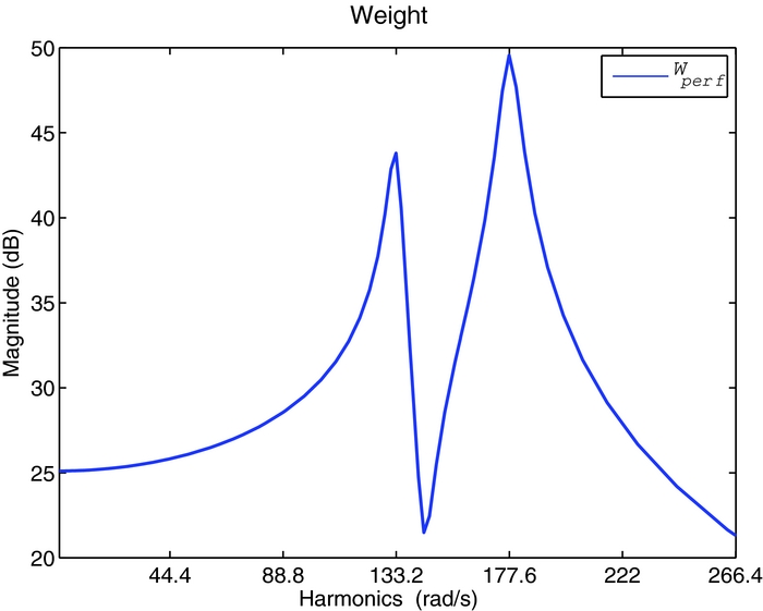
A constant (1 × 6) static gain matrix K is chosen for the control law. Since the dynamic model of the blade is already stable, the initial solution for the optimisation procedure can be assumed as the null matrix. The performance specification has been adapted to achieve satisfactory results, resulting in a decrease of the weight effect on the 4/rev harmonic; the hand-tuned frequency weighting function Wperf
, shown in Fig. 9, is similar to the H
2 controller weighting function of Fig. 8. The performance weighting matrix Q
k
of the cost function J is the identity matrix, because the performance specifications have been taken into account by Wperf
, and is kept constant for the whole period. The weight matrix
 $\mathbf{\mathbf{R}}_{k}$
, that prescribes further limitation for the control signal, is tuned until satisfactory loads reduction is achieved. In this example, it has a value of 5,000. The design of this controller is faster than that of the H
2 one because of the smaller number of parameters involved in the optimisation and because the solution of the two DPLEs is less demanding than the solution of the DTPREs(Reference Varga42).
$\mathbf{\mathbf{R}}_{k}$
, that prescribes further limitation for the control signal, is tuned until satisfactory loads reduction is achieved. In this example, it has a value of 5,000. The design of this controller is faster than that of the H
2 one because of the smaller number of parameters involved in the optimisation and because the solution of the two DPLEs is less demanding than the solution of the DTPREs(Reference Varga42).
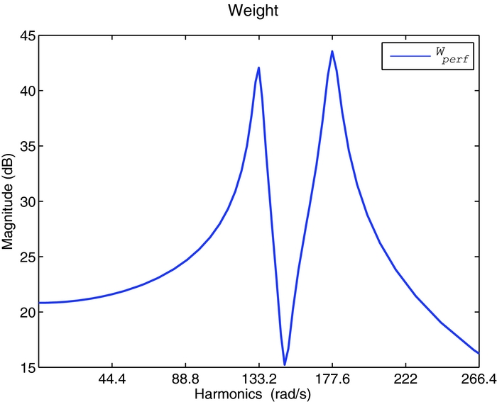
Figure 9. POF Control performance weight.
4.0 SIMULATION RESULTS
4.1 Closed-loop analysis on the design model
The performance of the periodic controllers, designed on the multi-body rotor model with low-fidelity aerodynamics, are shown at μ = 0.23. The periodic controllers are implemented in Simulink environment using S-functions. Rate-transition blocks are used before and after the controller because of the different sample times between the multi-body simulation and the periodic controller.
The vibration reduction achieved by the periodic controllers are summarised in Fig. 10. Although a significant passive load reduction is obtained by simply replacing the Bo 105 blades with the piezoelectric ones, both controllers allow to further alleviate the hub loads. The H 2 controller reduces the 4/rev harmonic of the hub force and moments FZ, MX and MY by 24%, 60% and 86%, respectively. The static output feedback controller achieve a reduction of 43%, 65% and 58%. Both solutions are satisfactory, and their performances are comparable. The H 2 controller has a better capability to reduce the moment MY , while the direct output feedback approach better alleviates FZ . On the average, the simpler static output feedback controller can be a valid substitute of the H 2 controller dynamic compensator, despite its faster algorithm and fewer design parameters. Note also that harmonics higher than the 4/rev are only marginally excited.
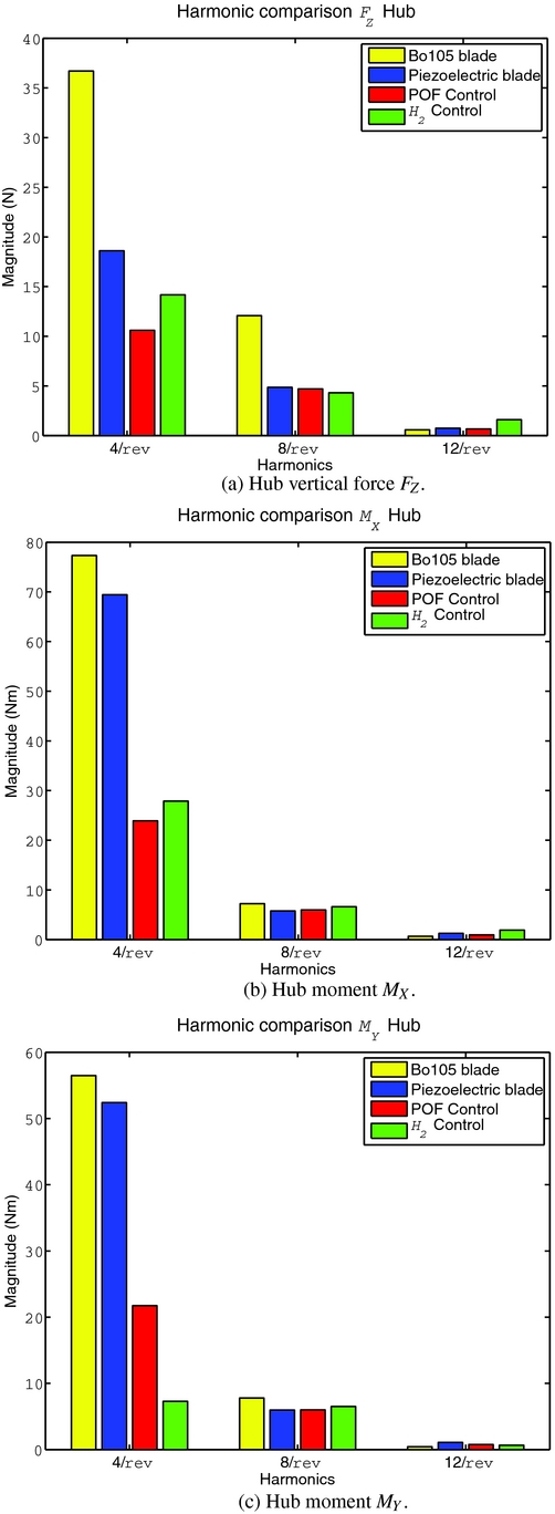
Figure 10. Vibrations reduction on the low-fidelity model at μ = 0.23.
The voltage applied on the first blade is shown in Fig. 11. The control signal is a sequence of steps because of the controller sampling time. The control effort remains quite low and does not exceed 80 V in both simulations. Note also that the control voltage computed by the static output feedback control has a lower-frequency content than that of the H 2 dynamic compensator; this may lead to better robustness properties, since it does not excite high-frequency harmonics that may not have been considered in the controller design phase.
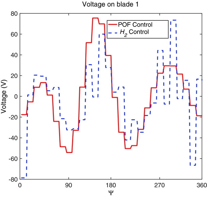
Figure 11. Applied voltage on blade 1 at μ = 0.23, design model.
4.2 Controller robustness validation
In this section, the periodic controllers designed using the simple aerodynamic model are tested with the model coupled with the free-wake code. Figure 12 shows the computed rotor wake and the non-dimensional inflow for the baseline condition. Dealing with the time-marching wake of the tip vortexes, it is possible to model the blade vortex interaction and to have a good approximation of the induced velocity of the rotor. This validation model is a useful test-bed for robustness validation because the dynamics of the blades is different, since the swashplate setting is changed to reach the same trim configuration of the previous model. Furthermore, the induced velocity, that is better approximated, increases the harmonic content of the aerodynamic loads. In fact, the baseline loads of Fig. 13, estimated with the free-wake model, are 1 order of magnitude higher than those of Fig. 10, that were estimated with the simple inflow model.
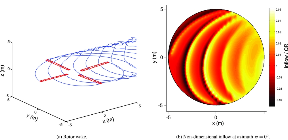
Figure 12. Free-wake aerodynamics (baseline condition at μ = 0.23).
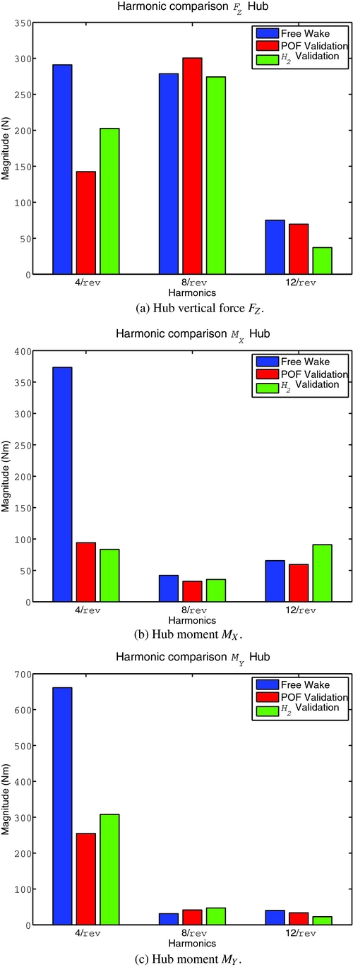
Figure 13. Validation of the controllers on the free-wake model using the piezoelectric blade.
Even if the improved aerodynamic model introduces new dynamics and raises the hub loads, none of the two controllers destabilise the rotor system, and they both achieve a good reduction of the loads. Both controllers reduce by more than 75% the moment MX of Fig. 13(b). The static output feedback controller seems to be more robust with respect to the force FZ of Fig. 13(b), and allows a larger reduction than that of the H 2 controller. This behaviour could be explained by the fact that the H 2 control leads to an augmented periodic state-space dynamic system with many controller parameters to be designed and additional dynamics in the closed-loop system. On the contrary, the direct output feedback control law is based on a simple gain matrix that is kept constant throughout the period of the system.
Figure 14 shows the applied control voltage. The control activity is significantly higher than that of Fig. 11 because of the higher loads; still, it remains bounded and acceptable, since it is not higher than 800 V. This somewhat high voltage for control purposes may be a problem for crew safety. It is however within the range of what can be found in the literature. For example, in Ref. 2 the active twist blades are excited with an amplitude of 1,000 V to assess vibrations reduction capabilities, while in Ref. 45 a voltage of ± 500 V is applied for blade de-icing.
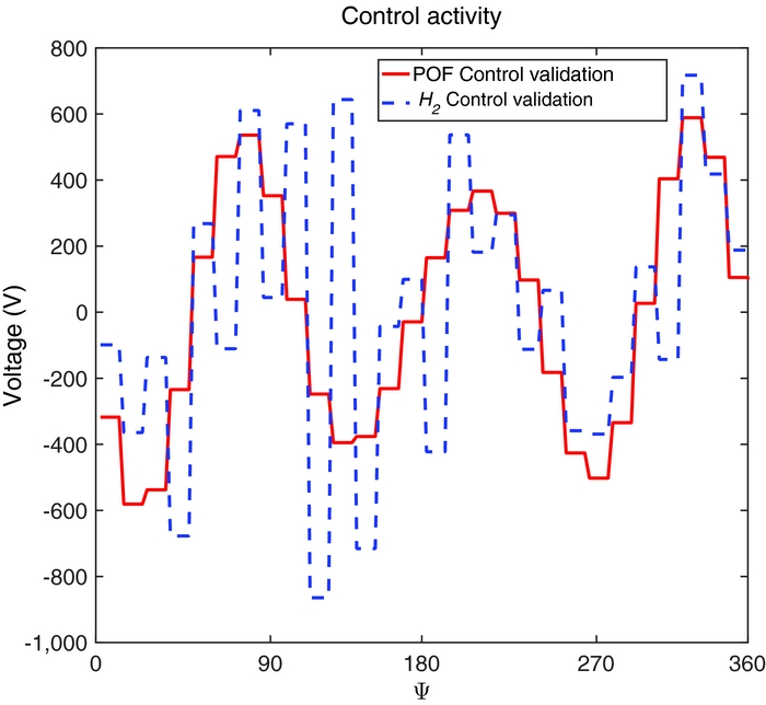
Figure 14. Applied voltage on blade 1 in the validation phase, μ = 0.23, free wake.
5.0 CONCLUSIONS
A multi-body numerical model of the Bo 105 main rotor is modified by adding actively twisted blades and used to design and implement individual blade control for hub vibration reduction relying on the periodic control theory. After identifying a periodic linearised model of the blade response, both the dynamic compensator arising from the H 2 periodic control theory and the periodic static output feedback controller, which minimise the 3/rev and the 4/rev harmonics of the blade root shear force, have been designed and tested. The closed-loop simulations are carried out by coupling MBDyn and Simulink. The controllers are validated on a more sophisticated free-wake aerodynamic model.
The design model shows a significant vibratory loads reduction with a small control effort, especially for the two hub moments MX and MY . Furthermore, the performance of the two periodic controller appears to be similar. This means that the direct periodic output feedback, which involves fewer design parameters and has a faster design algorithm, can be a valid substitute of the optimal H 2 approach. Moreover, using only a gain matrix in the control law would allow covering the entire flight envelope by simply interpolating, with a gain scheduling technique, the gain matrices. It would thus be possible to avoid the problems that could arise when interpolating state-space models(Reference Amsallem46,Reference Caigny, Camino and Swevers47) .
The validation model, with the free-wake aerodynamic code, shows that taking into account the periodicity of the rotor in forward flight leads to robust controllers even if model uncertainties are not considered in the design phase. In fact, there is no spill-over, and both of the controllers manage to reduce vibratory loads with satisfactory performance. These results seems promising for a practical implementation of such controllers.
It must be noted, however, that the robustness of these periodic controllers still has to be thoroughly investigated for a large number of trim configurations. The effectiveness of the envisioned static output feedback gain scheduling has also to be assessed.
A.0 APPENDIX
Controller Matrices Reconstruction
The controller matrices A C k , B C k , C C k and D C k of Equation (3.11) can be computed by following the procedure outlined in(Reference Ulker13) and reported here for completeness. It can be derived by the filtering and control theory in H 2 described in(Reference Bittanti and Colaneri40) by combining the observer and the full information state feedback control.
After solving the two periodic Riccati Equations (3.9) and (3.10), the sought matrices are given by:
 $$\begin{eqnarray}
\mathbf{A}_{k}^{C} =\mathbf{A}_{k}-\mathbf{L}_{k}\mathbf{C}_{2_{k}}+\mathbf{B}_{2_{k}}\mathbf{K}_{k}-\mathbf{B}_{2_{k}}\mathbf{L}_{k}^{O}\mathbf{C}_{2_{k}},
\end{eqnarray}$$
$$\begin{eqnarray}
\mathbf{A}_{k}^{C} =\mathbf{A}_{k}-\mathbf{L}_{k}\mathbf{C}_{2_{k}}+\mathbf{B}_{2_{k}}\mathbf{K}_{k}-\mathbf{B}_{2_{k}}\mathbf{L}_{k}^{O}\mathbf{C}_{2_{k}},
\end{eqnarray}$$
 $$\begin{eqnarray}
\mathbf{B}_{k}^{C} & =\mathbf{L}_{k}+\mathbf{B}_{2_{k}}\mathbf{L}_{k}^{O},
\end{eqnarray}$$
$$\begin{eqnarray}
\mathbf{B}_{k}^{C} & =\mathbf{L}_{k}+\mathbf{B}_{2_{k}}\mathbf{L}_{k}^{O},
\end{eqnarray}$$
 $$\begin{eqnarray}
\mathbf{C}_{k}^{C} & =\mathbf{K}_{k}-\mathbf{L}_{k}^{O}\mathbf{C}_{2_{k}},
\end{eqnarray}$$
$$\begin{eqnarray}
\mathbf{C}_{k}^{C} & =\mathbf{K}_{k}-\mathbf{L}_{k}^{O}\mathbf{C}_{2_{k}},
\end{eqnarray}$$
 $$\begin{eqnarray}
\mathbf{D}_{k}^{C} & =\mathbf{L}_{k}^{O},
\end{eqnarray}$$
$$\begin{eqnarray}
\mathbf{D}_{k}^{C} & =\mathbf{L}_{k}^{O},
\end{eqnarray}$$
where
 $$\begin{eqnarray}
\mathbf{L}_{k} =\left(\mathbf{A}_{k}\mathbf{Q}_{k}\mathbf{C}_{2_{k}}^{T}+\mathbf{B}_{1_{k}}\mathbf{D}_{21_{k}}^{T}\right)\left(\mathbf{C}_{2_{k}}\mathbf{Q}_{k}\mathbf{C}_{2_{k}}^{T}+\mathbf{D}_{21_{k}}\mathbf{D}_{21_{k}}^{T}\right)^{-1},
\end{eqnarray}$$
$$\begin{eqnarray}
\mathbf{L}_{k} =\left(\mathbf{A}_{k}\mathbf{Q}_{k}\mathbf{C}_{2_{k}}^{T}+\mathbf{B}_{1_{k}}\mathbf{D}_{21_{k}}^{T}\right)\left(\mathbf{C}_{2_{k}}\mathbf{Q}_{k}\mathbf{C}_{2_{k}}^{T}+\mathbf{D}_{21_{k}}\mathbf{D}_{21_{k}}^{T}\right)^{-1},
\end{eqnarray}$$
 $$\begin{eqnarray}
\mathbf{L}_{k}^{O} & =\left(\mathbf{K}_{k}\mathbf{Q}_{k}\mathbf{C}_{2_{k}}^{T}+\mathbf{W}_{k}\mathbf{D}_{21_{k}}^{T}\right)\left(\mathbf{C}_{2_{k}}\mathbf{Q}_{k}\mathbf{C}_{2_{k}}^{T}+\mathbf{D}_{21_{k}}\mathbf{D}_{21_{k}}^{T}\right)^{-1},
\end{eqnarray}$$
$$\begin{eqnarray}
\mathbf{L}_{k}^{O} & =\left(\mathbf{K}_{k}\mathbf{Q}_{k}\mathbf{C}_{2_{k}}^{T}+\mathbf{W}_{k}\mathbf{D}_{21_{k}}^{T}\right)\left(\mathbf{C}_{2_{k}}\mathbf{Q}_{k}\mathbf{C}_{2_{k}}^{T}+\mathbf{D}_{21_{k}}\mathbf{D}_{21_{k}}^{T}\right)^{-1},
\end{eqnarray}$$
 $$\begin{eqnarray}
\mathbf{K}_{k} & =-\left(\mathbf{B}_{2_{k}}^{T}\mathbf{P}_{k+1}\mathbf{B}_{2_{k}}+\mathbf{D}_{12_{k}}^{T}\mathbf{D}_{12_{k}}\right)^{-1}\left(\mathbf{B}_{2_{k}}^{T}\mathbf{P}_{k+1}\mathbf{A}_{k}+\mathbf{D}_{12_{k}}^{T}\mathbf{C}_{1_{k}}\right)
\end{eqnarray}$$
$$\begin{eqnarray}
\mathbf{K}_{k} & =-\left(\mathbf{B}_{2_{k}}^{T}\mathbf{P}_{k+1}\mathbf{B}_{2_{k}}+\mathbf{D}_{12_{k}}^{T}\mathbf{D}_{12_{k}}\right)^{-1}\left(\mathbf{B}_{2_{k}}^{T}\mathbf{P}_{k+1}\mathbf{A}_{k}+\mathbf{D}_{12_{k}}^{T}\mathbf{C}_{1_{k}}\right)
\end{eqnarray}$$
and
 $$\begin{equation}
\mathbf{W}_{k}=-\left(\mathbf{B}_{2_{k}}^{T}\mathbf{P}_{k+1}\mathbf{B}_{2_{k}}+\mathbf{D}_{12_{k}}^{T}\mathbf{D}_{12_{k}}\right)^{-1}\left(\mathbf{B}_{2_{k}}^{T}\mathbf{P}_{k+1}\mathbf{B}_{1_{k}}+\mathbf{D}_{12_{k}}^{T}\mathbf{D}_{11_{k}}\right).
\end{equation}$$
$$\begin{equation}
\mathbf{W}_{k}=-\left(\mathbf{B}_{2_{k}}^{T}\mathbf{P}_{k+1}\mathbf{B}_{2_{k}}+\mathbf{D}_{12_{k}}^{T}\mathbf{D}_{12_{k}}\right)^{-1}\left(\mathbf{B}_{2_{k}}^{T}\mathbf{P}_{k+1}\mathbf{B}_{1_{k}}+\mathbf{D}_{12_{k}}^{T}\mathbf{D}_{11_{k}}\right).
\end{equation}$$
Should matrix D 22 k be non-null, i.e. should direct feed-through be present, then the matrices would have to be modified into(Reference Zhou and Doyle48):
 $$\begin{eqnarray}
\tilde{\mathbf{A}}_{k}^{C} =\mathbf{A}_{k}^{C}-\mathbf{B}_{k}^{C}\mathbf{D}_{22_{k}}\mathbf{T}_{k}^{-1}\mathbf{C}_{k}^{C},
\end{eqnarray}$$
$$\begin{eqnarray}
\tilde{\mathbf{A}}_{k}^{C} =\mathbf{A}_{k}^{C}-\mathbf{B}_{k}^{C}\mathbf{D}_{22_{k}}\mathbf{T}_{k}^{-1}\mathbf{C}_{k}^{C},
\end{eqnarray}$$
 $$\begin{eqnarray}
\tilde{\mathbf{B}}_{k}^{C} & =\mathbf{B}_{k}^{C}-\mathbf{B}_{k}^{C}\mathbf{D}_{22_{k}}\mathbf{T}_{k}^{-1}\mathbf{D}_{k}^{C},
\end{eqnarray}$$
$$\begin{eqnarray}
\tilde{\mathbf{B}}_{k}^{C} & =\mathbf{B}_{k}^{C}-\mathbf{B}_{k}^{C}\mathbf{D}_{22_{k}}\mathbf{T}_{k}^{-1}\mathbf{D}_{k}^{C},
\end{eqnarray}$$
 $$\begin{eqnarray}
\tilde{\mathbf{C}}_{k}^{C} & =\mathbf{T}_{k}^{-1}\mathbf{C}_{k}^{C},
\end{eqnarray}$$
$$\begin{eqnarray}
\tilde{\mathbf{C}}_{k}^{C} & =\mathbf{T}_{k}^{-1}\mathbf{C}_{k}^{C},
\end{eqnarray}$$
 $$\begin{eqnarray}
\tilde{\mathbf{D}}_{k}^{C} & =\mathbf{T}_{k}^{-1}\mathbf{D}_{k}^{C},
\end{eqnarray}$$
$$\begin{eqnarray}
\tilde{\mathbf{D}}_{k}^{C} & =\mathbf{T}_{k}^{-1}\mathbf{D}_{k}^{C},
\end{eqnarray}$$
where
 $$\begin{equation}
\mathbf{T}_{k}=\mathbf{D}_{k}^{C}\mathbf{D}_{22_{k}}+\mathbf{I}
\end{equation}$$
$$\begin{equation}
\mathbf{T}_{k}=\mathbf{D}_{k}^{C}\mathbf{D}_{22_{k}}+\mathbf{I}
\end{equation}$$
and I is the identity matrix.