NOMENCLATURE
- c
chord length
- C D
drag coefficient,
 $$C_{{\rm D}} {\equals}{D \over {q_{\infty} \cdot S}}$$
- (C D)ref
reference drag coefficient (baseline design)
- (C D)rel
normalised drag coefficient,
$$(C_{{\rm D}} )_{{{\rm rel}}} {\equals}{{C_{{\rm D}} } \over {\,\mid\,(C_{{\rm D}} )_{{{\rm ref}}} \,\mid\,}}$$
- C L
lift coefficient,
$$C_{{\rm L}} {\equals}{L \over {q_{\infty} \cdot S}}$$
- (C L)ref
reference lift coefficient (baseline design)
- (C L)rel
normalised lift coefficient,
$$(C_{{\rm L}} )_{{{\rm rel}}} {\equals}{{C_{{\rm L}} } \over {\,\mid\,(C_{{\rm L}} )_{{{\rm ref}}} \,\mid\,}}$$
- C p
pressure coefficient,
$$C_{{\rm p}} {\equals}{{p{\minus}p_{\infty} } \over {q_{\infty} }}$$
- d FFB
diameter of the full-fairing beanie
- D
drag
- f(x)
objective function
- l y
length of the blade-sleeve fairing in the y-direction
- L
lift
- M
Mach number
- n Rotor
rotor speed
- p ∞
ambient pressure
- q ∞
dynamic pressure,
$$q_{\infty} {\equals}{{\rho _{\infty} \cdot V_{\infty}^{2} } \over 2}$$
- r
radius
- R
rotor radius
- S
reference area
- S i
blade-sleeve fairing section
- Δt
time-step size
- t sim
simulation time
- T sim
total simulation time
- u τ
friction velocity,
$$u_{{\rm \tau }} {\equals}\sqrt {{\rm \tau }_{w} {\rm \rho }} $$
- V Cruise
cruise speed of the helicopter
- V X , mean
averaged, axial flow velocity
- V ∞
free-stream velocity
- x, y, z
Cartesian coordinates
- x
design variable vector
- y +
dimensionless wall distance,
$$y^{{\plus}} {\equals}{{u_{\tau } \cdot y} \over \nu }$$


GREEK SYMBOL
- v
kinematic viscosity
- Ψ
Azimuthal rotor blade positions
- ρ∞
density
- τ w
wall shear stress
1.0 INTRODUCTION
Europe and its aviation industry have defined very ambitious goals regarding the development of future air transportation concepts. The reduction of the environmental impact as well as the performance improvement of future vehicles are the key challenges to be tackled. Especially, the reduction in CO2 and NO x emissions as well as the decrease of the noise footprint are in focus. At the same time, a seamless door-to-door mobility is required by the growing population. However, conventional aircraft require a large ground infrastructure and rotorcraft do not achieve the cruising speed, payload and range of such an aircraft. Therefore, the gap between those two configurations can only be closed by the development of a novel aircraft concept. One of these concepts is represented by the new compound helicopter configuration known as Rapid And Cost-Effective Rotorcraft (RACER), which is developed within the European Clean Sky 2 Joint Technology Initiative (CS2-JTI). The RACER combines the beneficial characteristics of a fixed-wing aircraft with the ability of a helicopter for vertical take-off and landing (VTOL). Furthermore, the targeted cruising speed is around 220 kn, which is approximately 50% higher than for a conventional helicopter. Due to the high cruising speed, aerodynamic efficiency becomes an important topic during the RACER development. Regarding conventional helicopters, the rotor head represents a major drag source, which offers potential in terms of drag reduction. Hence, one possibility is to design fairings for certain rotor head components, which was comprehensively investigated within the Clean Sky Green RotorCraft Research Program( Reference Breitsamter, Grawunder and Reß 1 , Reference Desvigne and Alfano 2 ). Moreover, the importance of hub drag minimisation is reflected by a large number of experimental( Reference Graham, Sung, Young, Louie and Stroub 3 – Reference Sung, Lance, Young and Stroub 5 ) and numerical investigations( Reference Khier 6 , Reference Khier 7 ) that have been conducted over the last decades. The present work is related to the Clean Sky 2 project FURADO (Full Fairing Rotor Head Aerodynamic Design Optimisation), which deals with the aerodynamic design optimisation of a semi-watertight full-fairing rotor head by means of CFD simulations. For this purpose, the rotor-head fairings are divided into three main components: the blade-sleeve fairing (BSF), the full-fairing beanie and the pylon fairing. The present publication deals with the aerodynamic design optimisation of the RACER BSF. During preliminary work, 2D aerofoils were aerodynamically optimised for selected sections of the BSF. These aerofoils yield a database of supporting geometries, which are used for the modification of the 3D fairing shape. Furthermore, a global multi-objective genetic optimisation algorithm is applied and selected supporting aerofoils represent the design variables for the given optimisation problem.
2.0 RACER COMPOUND HELICOPTER
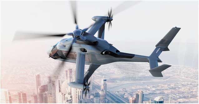
The innovative demonstrator RACER provides a concept allowing to expand the flight envelope of helicopters towards higher cruising speeds. The development of this new configuration is based on the experience gained through the X3 demonstrator program of Airbus Helicopters( 8 ). It offers a common demonstrator platform for new technologies and it is developed within a European framework of industrial and academic partners. Figure 1 gives an overview on the RACER compound helicopter configuration. The main differences, compared to a conventional helicopter, are given by the innovative box-wing design holding two lateral rotors as well as the horizontal and vertical stabilisers in H-type architecture. Moreover, a classical five-bladed main rotor is used enabling vertical take-off and landing. Concerning cruise flight, a significant part of the lift is generated by the wings.

Figure 1. Clean Sky 2 demonstrator RACER( 9 ).
Hence, the main rotor can be unloaded and its rotational speed is decreased, which keeps the tip Mach-number of the advancing rotor blade (RB) low enough to avoid transonic effects. Furthermore, the stabilisers are equipped with rudders and provide pitch and yaw stability during cruise flight. The propellers deliver additional thrust, generate anti-torque and enable yaw control in hover.
The expected RACER performance is defined by a 50% higher cruising speed and a cost reduction of 25% per nautical mile compared to conventional helicopters from the same class( 9 ). In order to achieve the predicted goals, drag reduction is one of the major challenges to be tackled during the RACER development. Therefore, highly efficient wings, a low-drag fuselage and a fully faired main rotor are employed.
3.0 GEOMETRY PARAMETERISATION
Within the present publication, the aerodynamic design optimisation of the RACER BSF is at focus. Figure 2 shows a simplified CAD model of the investigated rotor head, which consists of three components. These include the full-fairing beanie (FFB) in green, the BSF in orange and a truncated RB in blue. Hence, an isolated rotor head is taken into account and its interference effects with the fuselage as well as the pylon fairing are neglected. Additionally, the dampers between the RBs are omitted, which provides a watertight surface and reduces the complexity in terms of mesh generation. Furthermore, an undisturbed inflow is obtained for all blade-sleeve sections, which allows for the definition of specific free-stream conditions. The junction between the BSF and the full-fairing beanie as well as the transition to the RB are geometrically fixed. Hence, these sections keep their shape throughout the optimisation process. Furthermore, the cross-sections of the supporting aerofoils, which represent the basis for the 3D BSF, are depicted in Fig. 2. The shape variation of the BSF is achieved by replacing the supporting aerofoils. For this purpose, a database of selected 2D geometries is employed, which was generated during previous work within the FURADO project(
Reference Pölzlbauer, Desvigne and Breitsamter
10
). The four supporting aerofoils (S1–S4) are located in a region of
 $$0.078\leq r\,/\,R\leq 0.149$$
, where R corresponds to the rotor radius.
$$0.078\leq r\,/\,R\leq 0.149$$
, where R corresponds to the rotor radius.
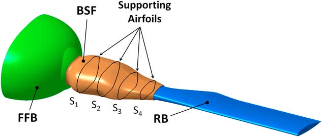
Figure 2. CAD model applied for the design optimisation of the RACER blade-sleeve fairing (baseline design).
The generation of the 3D BSF is based on a supporting structure, which is given in Fig. 3. The four replaceable aerofoils (S1–S4) are illustrated by blue lines and the geometrically fixed sections are shown by black lines. The green supporting curves consist of splines and straight lines that are connected through prescribed points. The axial positions of these points were defined in order to fulfil mounting requirements. Furthermore, all splines are set tangential to the straight supporting curves between S1 and S2. The surface of the BSF consists of four tangential sub-surfaces in the front, back, top and bottom. Regarding the automated shape generation using CATIA V5R21, a parameterised CAD model is applied in combination with a design table. Depending on the selected set of supporting aerofoils, the design table is actualised and the CAD model is updated using a predefined CATIA macro.
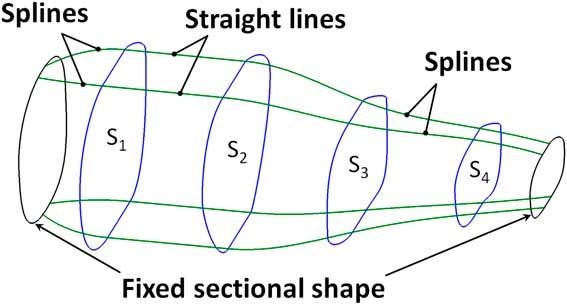
Figure 3. Supporting structure for the surface generation (baseline design).
4.0 OPTIMISATION APPROACH
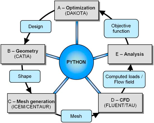
Within this section, the aerodynamic design optimisation process for the RACER BSF is described. This includes an introduction to the applied optimisation tool chain, a description of the optimisation problem and a brief overview on the selected optimisation algorithm. A general introduction to optimisation formulation and different optimisation techniques is given in Ref. 11. During the first phase of the FURADO project, the optimisation tool chain allowing for fully automated aerodynamic shape optimisation was developed. It consists of five main modules, which are illustrated in Fig. 4. These modules can be divided into optimisation, shape generation, mesh generation, flow simulation and design evaluation. The tool chain contains several commercial as well as non-commercial software packages and a detailed description is provided in Ref. 10.

Figure 4. Optimisation tool chain allowing for automated shape development( Reference Pölzlbauer, Desvigne and Breitsamter 10 ).
4.1 Optimisation problem
Regarding the current optimisation problem, the geometry of Fig. 2 is examined. During preliminary work, the supporting aerofoils (S1–S4) were aerodynamically optimised for cruise flight, which is the most relevant flight condition in terms of drag reduction( Reference Pölzlbauer, Desvigne and Breitsamter 10 ). For this purpose, the local flow conditions for each section were taken into account, which vary due to the circumferential velocity of the rotor and the flow deflection caused by the fuselage. Two different azimuthal positions of the rotor were investigated, which are shown in Fig. 5 and correspond to the advancing and the retreating RB. Previous investigations at TUM-AER revealed that the highest drag values are obtained at these azimuthal rotor positions( Reference Grawunder, Reß, Stein, Breitsamter and Adams 12 ). Typical flow-velocity profiles for cruise flight are given in Fig. 5(a) and (b). The flow conditions are characterised by high Mach numbers in the tip region of the advancing RB and a reverse-flow region in the vicinity of the rotor axis for the retreating RB.

Figure 5. Comparison of the flow conditions for the investigated azimuthal rotor positions.
Regarding the RACER demonstrator, the rotational speed of the main rotor is adapted for each flight condition to keep the tip Mach number within a permissible range during cruise flight and to provide sufficient lift during hover.
The design optimisation of the 2D blade-sleeve sections (S1–S4) was conducted using a multi-objective genetic algorithm with two objective functions. The theory about genetic optimisation algorithms is described in Section 4.2. The applied objective functions included the maximisation of the lift-to-drag ratio for the advancing blade case and the minimisation of the drag coefficient for the retreating blade case. Regarding the parameterisation of the two-dimensional shapes, third-order Bézier curves( Reference Böhm, Farin and Kahmann 13 – Reference Sederberg 15 ) were applied and the design variables were given by the coordinates of the Bézier control points. The application of a genetic optimisation algorithm leads to a large database of optimised shapes for each section. This allows for the selection of relevant geometries from the Pareto front of the final population. Hence, a prescribed set of sectional shapes (S1–S4) is used for the present optimisation task. Since the 2D design optimisation of the blade-sleeve sections represents the basis for the current work, similar objective functions are applied and their mathematical description is given by Equations (1) and (2). The main objective is to reduce the drag caused by the BSFs during cruise flight. However, lift is taken into account as well in the objective function for the advancing RB. In terms of overall drag, any additional lift generated by the BSFs would have a beneficial effect on the entire configuration. Moreover, the minimisation of drag is considered as the objective function for the retreating RB, which is located within a region of reversed flow:
 $${\rm maximise}\;f_{1} ({\bf x}){\equals}C_{{\rm L}} \,/\,C_{{\rm D}} \,({\rm advancing}\,{\rm blade})$$
 $$\ {\rm minimise}\;f_{2} ({\bf x}){\equals}C_{{\rm D}} \cdot S\,({\rm retreating}\,{\rm blade})$$
Four discrete design variables representing specific geometries of the supporting aerofoils are applied:
 $${\bf x}{\equals}\{ S_{1} ,S_{2} ,S_{3} ,S_{4} \} \,{\rm with}\,\{ S_{i} \in{\Bbb Z}\quad \,\mid\,\quad 1\leq S_{i} \leq 12\} $$
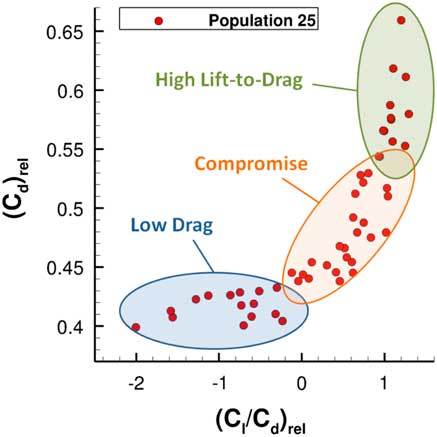
For each section (S1–S4), 12 shapes originating from the 2D design optimisation are selected. The sectional shapes are parameterised by third-order Bézier curves and each selected design represents a prescribed set of coordinates for the Bézier control points. Figure 6 exemplarily shows the objective space for the final population of one blade-sleeve section. Both objective functions are normalised by reference values of a symmetric reference geometry. The designs close to the Pareto front can be divided into three main regions. Designs with low drag values regarding the retreating blade case are located in the blue coloured region and geometries offering a compromise between both objective functions can be found in the orange coloured region. Moreover, the green coloured region contains designs with high lift-to-drag ratios concerning the advancing blade case. From each of the three regions, four aerofoils are selected for each of the blade-sleeve sections yielding the design variables for the present optimisation task. Hence, a database containing 48 optimised aerofoils is created, which corresponds to 20,736 possible shape combinations.

Figure 6. Exemplary objective space for the final population of the 2D design optimisation showing the three main regions of the Pareto front.
Evaluating all possible shapes of the BSF is not possible within a reasonable time-frame. Additionally, the modality and the characteristics of the design space are unknown. Therefore, a robust multi-objective genetic optimisation algorithm is employed to find feasible geometries for the RACER BSF. During the preliminary optimisation of the blade-sleeve sections, design constraints regarding the available design space were applied. Therefore, these constraints should automatically be met by the three-dimensional BSF and an unconstrained optimisation can be performed. However, slight violations due to the interpolation between the blade-sleeve sections could occur and a manual check of the design constraints is necessary for designs of interest.
4.2 Optimisation algorithm
The selection of the optimisation algorithm for a given optimisation problem is based on the characteristics of the design space and the applied constraints. In convex search spaces, gradient-based optimisation algorithms efficiently navigate into a local optimum close to the starting point. However, these algorithms are not suited for multi-modal problems, because they could get caught in such a local optimum. Therefore, derivative-free global evolutionary algorithms offer a robust alternative in non-convex search spaces or whenever the characteristics of the search space are unknown. However, global optimisation algorithms require a large number of function evaluations compared to gradient-based algorithms. Concerning the present optimisation problem, similar concurring objective functions as for the 2D design optimisation are employed. However, they slightly differ, because the force-coefficients are multiplied by the reference surface S for the 3D investigations. Moreover, the flow around the rotor head fairing represents a complex flow problem and the properties of the search space are unknown. Therefore, a robust multi-objective genetic algorithm (MOGA) is used for the aerodynamic design optimisation of the RACER BSF. Genetic algorithms (GAs) use the principles of natural selection, which means that they are based on Darwin’s theory of survival of the fittest. These algorithms start their search for the optimal solutions from a population of designs and not from a single one. In combination with a parameter sampling method, which is applied for the initialisation of the first population, a wide range of the design space can already be covered at the beginning of the optimisation process. Moreover, GAs only use objective functions to determine the fitness of a design. Hence, they do not require any auxiliary information, like gradients or Hessians. The transition from one population to a subsequent one depends on probabilistic rules. The main operations used within a GA are reproduction, crossover and mutation. Depending on the objective function of a candidate, it has a certain probability of being selected for contributing offspring in the next generation. Within the next step, a mating pool of candidates is generated and they are combined in pairs crossing over genetic information. Additionally, a mutation operator is employed to randomly change the values of coded design variable strings in order to prevent the optimisation algorithm from losing important genetic information( Reference Goldberg 16 , Reference Kalyanmoy 17 ).
5.0 NUMERICAL SETUP
Within this section, an overview on the investigated flow conditions, the computational mesh and the applied flow solvers is given. As mentioned in Section 4.1, two different flow conditions are examined yielding the advancing and the retreating RB case (Ψ=90° and Ψ=270°). In order to simplify the optimisation process, a single RB is investigated at these fixed azimuthal rotor positions using the geometry of Fig. 2. This simplification significantly reduces the computational effort and allows for the evaluation of a large number of designs within a reasonable time frame. Nevertheless, the influence of the circumferential velocity has to be taken into account within the flow simulations. Therefore, the rotational speed of the rotor is considered by a single value of the circumferential velocity, which represents the average value of all blade-sleeve sections. This approximation can be done, because the radial distance between the first (S1) and the last section (S4) is rather small.
Hence, the freestream velocities for the advancing and the retreating blade case are calculated by superposing the averaged circumferential velocity with the cruise speed of the helicopter, which corresponds to V Cruise=220 kn. Furthermore, an averaged angle-of-attack is applied, which is defined by the collective pitch, the longitudinal cyclic-pitch and an averaged local angle-of-attack due to the flow deflection of the fuselage. Additionally, the employed ambient conditions are representative for a sea-level cruise flight in ICAO standard atmosphere( Reference Organization 18 ). Due to the fact that an isolated RB is investigated at fixed azimuthal positions, simplified flow conditions are assumed. Any interactional effects with preceding RBs are neglected and the vertical flow field is not predicted correctly. However, the presented approach offers a rapid preliminary design optimisation of the BSF and allows for the preselection of promising designs. These designs will be assessed in more detail within a subsequent step and the influence of 3D effects will be highlighted. For this purpose, hover as well as forward flight will be investigated considering the full RACER configuration with the optimised fairings and a rotating rotor head.
5.1 Computational mesh
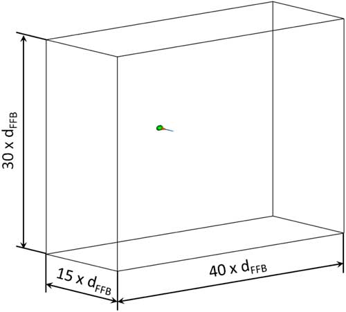
The applied computational mesh is generated with Ansys ICEM. A block-structured hexahedral mesh consisting out of 182 blocks is created. The dimensions of the computational domain are illustrated in Fig. 7. The quantity dFFB represents the diameter of the full-fairing beanie, which is shown in green. The size of the domain is big enough to ensure that no influence from the imposed boundary conditions can be observed in the flow field near the geometry. In order to minimise the computational time, on the one hand, and to ensure low numerical dissipation due to the spatial discretisation, on the other hand, mesh independence studies were conducted to find the required mesh size. As a result, a computational mesh featuring 7.2 m elements was selected for the numerical investigations. Furthermore, the boundary-layer is fully resolved by selecting a dimensionless wall distance of y+≈1 for the initial cell height and a mesh expansion ratio of 1.2. On the front, top, back and bottom of the computational domain, farfield boundary conditions are applied. A symmetry boundary condition is used on the surface connected to the investigated geometry. For the remaining side of the domain, a free-slip wall is chosen. The initial mesh is generated for a baseline geometry of the BSF, which uses aerofoils yielding the best compromise of both objective functions. Subsequent meshes are automatically generated by updating the geometries and re-association.

Figure 7. Computational domain used for the CFD simulations.
5.2 Flow solvers
This section summarises the numerical setup of the applied flow solvers. Ansys FLUENT as well as the DLR TAU-Code were used for the numerical investigations within the present publication. The preliminary aerodynamic design optimisation of the BSF sections was conducted using Ansys FLUENT, because faster convergence was observed in terms of unsteady flow simulations. Therefore, all time-accurate results for detailed analysis were produced with this flow solver. Regarding the currently ongoing 3D design optimisation, steady-state flow simulations are performed with the DLR TAU-Code. The selection of the steady-state simulation setup is justified by comparison to a time-accurate flow simulation.
5.2.1 Ansys FLUENT
The numerical flow simulations dealing with the 2D design optimisation of the BSF sections were conducted with Ansys FLUENT. Furthermore, selected 3D BSF designs were investigated with this flow solver. Due to free-stream Mach numbers within a range of 0.3–0.4, compressibility effects are taken into account. Therefore, the compressible, unsteady Reynolds-Averaged Navier–Stokes equations (URANS) are considered. The initialisation of the transient flow simulation is performed by the application of a steady state solution. Furthermore, the k−ω SST model(
Reference Menter
19
) is employed for turbulence modelling. Moreover, the SIMPLEC algorithm is applied for the treatment of pressure–velocity coupling, which allows for increased under-relaxation. The pressure interpolation is achieved by the standard pressure scheme of FLUENT. Regarding the spatial discretisation, second-order upwind schemes are chosen for density, momentum, turbulent kinetic energy, specific dissipation rate and energy. Further, a least-squares cell-based formulation is applied for the gradient calculation and a bounded second-order implicit scheme is used for the temporal discretisation(
20
). The time-step size for the time-accurate simulations was set to
 $$\Delta t {\equals} 1{\times}10^{{{\minus}4}} {\rm s}$$
, which corresponds to a resolution of 130 points per period regarding the observed oscillation of forces. Furthermore, all normalised residuals were reduced by at least four orders of magnitude. Depending on the investigated geometry, this was achieved within approximately ten inner iterations per time step. During preliminary tests regarding the simulation setup, it was observed that doubling the time-step size leads to approximately 60% more inner iterations and a more stable setup could be obtained with the smaller time-step. The applied fluid is air ideal gas and its properties are set according to a sea-level cruise flight.
$$\Delta t {\equals} 1{\times}10^{{{\minus}4}} {\rm s}$$
, which corresponds to a resolution of 130 points per period regarding the observed oscillation of forces. Furthermore, all normalised residuals were reduced by at least four orders of magnitude. Depending on the investigated geometry, this was achieved within approximately ten inner iterations per time step. During preliminary tests regarding the simulation setup, it was observed that doubling the time-step size leads to approximately 60% more inner iterations and a more stable setup could be obtained with the smaller time-step. The applied fluid is air ideal gas and its properties are set according to a sea-level cruise flight.
5.2.2 DLR TAU-Code
The numerical investigations for the evaluation of the objective functions concerning the three-dimensional design optimisation are conducted with the DLR-TAU Code. This CFD solver was developed at the DLR (German Aerospace Center) and solves the compressible steady or unsteady Reynolds-Averaged Navier–Stokes (RANS) equations. The flow calculation is based on a dual grid approach and a cell vertex grid metric is employed. Turbulence modelling is achieved by the SST k–g model, which represents a re-implemented version of the Menter SST model( Reference Menter 19 , Reference Lakshmipathy and Togiti 21 ). The standard TAU average of flux central scheme is selected for the discretisation of the meanflow equations. Furthermore, a Roe second-order scheme is applied for the convective fluxes of the turbulence equations and a Green–Gauss algorithm is chosen for the gradient reconstruction. The system of equations is solved by a Lower-Upper Symmetric-Gauss–Seidel (LU-SGS) method and scalar dissipation is used for the numerical dissipation scheme. An overview of the hybrid RANS solver TAU is given in Ref. 22. Regarding the convergence of the flow simulations, the normalised density residual was reduced by four orders of magnitude. However, the convergence behaviour depends on the investigated geometry.
6.0 RESULTS
The present section introduces the applied optimisation setup and shows the intermediate results of the currently ongoing BSF optimisation. The Automated Aerodynamic Shape Development (AASD) tool chain, which was developed at TUM-AER, was used in combination with a multi-objective genetic algorithm to generate the data. The investigated objective functions are given by the maximisation of the lift-to-drag ratio (C
L/C
D) for the advancing RB (Ψ=90°) and the minimisation of drag C
DS for the retreating RB (Ψ=270°), where Ψ is the RB azimuth measured from the back blade location. Four discrete design variables, which correspond to specific designs from an aerofoil database, span the available design space. Twelve aerofoils were selected for each section, which yields a design variable range of
 $$1\leq {\rm S}_{1} ,{\rm S}_{2} ,{\rm S}_{3} ,{\rm S}_{4} \leq 12$$
. Regarding the ranking of the designs, a domination count is used to order the population members and to determine their fitness. One design is dominating another one, if it is better in both objective functions. The designs that are kept for the subsequent generation are selected by a below limit replacement value of six. This means that the number of candidates dominating a specific design has to be lower than the replacement value, otherwise this design is rejected. Furthermore, the reduction of the population size is controlled by a shrinkage percentage of 95%. This value specifies the number of candidates, which have to continue to the next generation. Hence, it prevents an excessive decrease in the population size. Furthermore, the below-limit selector is adapted, if the algorithm does not find sufficient designs to fulfil the shrinkage percentage requirement. Additionally, a differentiation along the Pareto-frontier is achieved by employing niching during the optimisation. The initial population contains 150 designs, which were randomly generated by the applied optimisation tool-box DAKOTA(
Reference Adams, Ebeida, Eldred, Jakeman, Maupin and Monschke
23
). Regarding the optimisation results, an evaluation of the objective space is conducted and one design is selected to be investigated in more detail. Moreover, an overview on the prevailing flow field is given and the occurring flow phenomena are described.
$$1\leq {\rm S}_{1} ,{\rm S}_{2} ,{\rm S}_{3} ,{\rm S}_{4} \leq 12$$
. Regarding the ranking of the designs, a domination count is used to order the population members and to determine their fitness. One design is dominating another one, if it is better in both objective functions. The designs that are kept for the subsequent generation are selected by a below limit replacement value of six. This means that the number of candidates dominating a specific design has to be lower than the replacement value, otherwise this design is rejected. Furthermore, the reduction of the population size is controlled by a shrinkage percentage of 95%. This value specifies the number of candidates, which have to continue to the next generation. Hence, it prevents an excessive decrease in the population size. Furthermore, the below-limit selector is adapted, if the algorithm does not find sufficient designs to fulfil the shrinkage percentage requirement. Additionally, a differentiation along the Pareto-frontier is achieved by employing niching during the optimisation. The initial population contains 150 designs, which were randomly generated by the applied optimisation tool-box DAKOTA(
Reference Adams, Ebeida, Eldred, Jakeman, Maupin and Monschke
23
). Regarding the optimisation results, an evaluation of the objective space is conducted and one design is selected to be investigated in more detail. Moreover, an overview on the prevailing flow field is given and the occurring flow phenomena are described.
6.1 Baseline design
In order to provide a reference for the present optimisation task, a baseline geometry of the BSF is manually designed. The applied supporting aerofoils offer the best compromise between the objective functions from the 2D design optimisation. The baseline design of the BSF is depicted in Fig. 2 and the corresponding supporting geometries are shown in Fig. 3. The performance improvement of the optimised BSFs is measured relative to the baseline design.
6.2 Evaluation of the objective space
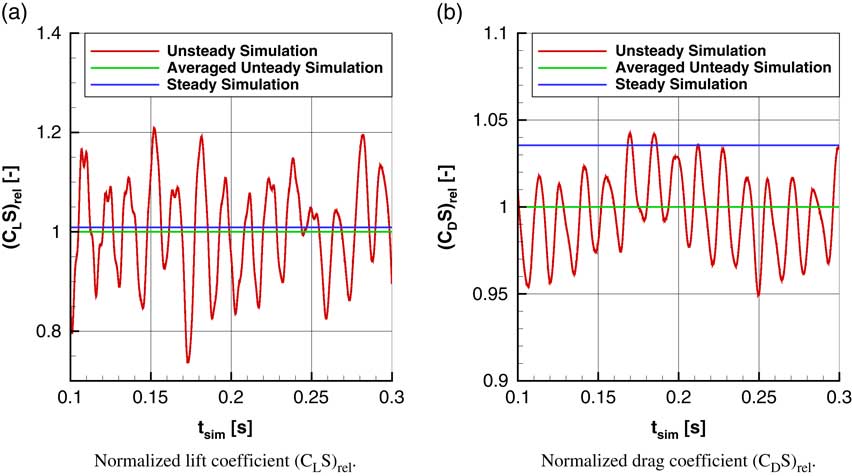
Within this section, the evaluation of the BSF designs is presented. The investigated geometry yields a bluff body and an unsteady flow field can be observed in its wake region. However, time-accurate flow simulations require a significant amount of time, which is undesired in terms of the automated design optimisation. Therefore, a comparison between a time-accurate and a steady-state flow simulation was conducted for a representative test-case using the DLR-TAU Code. Figure 8 shows the results for the time-accurate simulation (red), the averaged time-accurate simulation (green) and the steady-state simulation (blue). All results are normalised with the final value of the averaged time-accurate simulation. The total simulation time was T
sim=0.3 s and the applied time-step was
 $$\Delta t{\equals}2{\times}10^{{{\minus}4}} {\rm s}$$
. Regarding the normalised lift-coefficient (CLS)rel, which is illustrated in Fig. 8(a), a deviation of 0.9% can be observed between the steady-state and the averaged time-accurate simulation. Furthermore, a difference of 3.5% was obtained for the normalised drag-coefficient (C
D
S)rel, which is shown in Fig. 8(b). The deviation from the time-accurate simulation is considered to be within a reasonable range and therefore, a steady-state simulation setup is used for the current optimisation task.
$$\Delta t{\equals}2{\times}10^{{{\minus}4}} {\rm s}$$
. Regarding the normalised lift-coefficient (CLS)rel, which is illustrated in Fig. 8(a), a deviation of 0.9% can be observed between the steady-state and the averaged time-accurate simulation. Furthermore, a difference of 3.5% was obtained for the normalised drag-coefficient (C
D
S)rel, which is shown in Fig. 8(b). The deviation from the time-accurate simulation is considered to be within a reasonable range and therefore, a steady-state simulation setup is used for the current optimisation task.

Figure 8. Comparison of an averaged time-accurate flow simulation with the results from a quasi-steady-state flow simulation.
A steady-state flow simulation with 22,000 iterations is performed to calculate the objective functions for the design evaluation. During the first phase of the design optimisation, 334 designs have been evaluated. An overview on the objective space is given in Fig. 9. Both objective functions are normalised with reference values from the baseline design of the BSF. Hence, the performance of a candidate is evaluated relative to this reference geometry. The feasible objective space is defined in a region of
 $${\minus}0.63\leq (C_{{\rm L}} \,/\,C_{{\rm D}} )_{{{\rm rel}}} \leq 1.14$$
and
$${\minus}0.63\leq (C_{{\rm L}} \,/\,C_{{\rm D}} )_{{{\rm rel}}} \leq 1.14$$
and
 $$0.89\leq (C_{{\rm D}} S)_{{{\rm rel}}} \leq 1.2$$
. Furthermore, the baseline design, which is located at
$$0.89\leq (C_{{\rm D}} S)_{{{\rm rel}}} \leq 1.2$$
. Furthermore, the baseline design, which is located at
 $$(C_{{\rm L}} \,/\,C_{{\rm D}} )_{{{\rm rel}}} {\equals} 1$$
and
$$(C_{{\rm L}} \,/\,C_{{\rm D}} )_{{{\rm rel}}} {\equals} 1$$
and
 $$(C_{{\rm D}} S)_{{{\rm rel}}} {\equals} 1$$
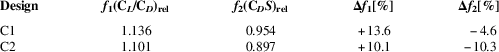
, is marked with a blue symbol. Any design that is better than the reference, is located within the highlighted region, in the bottom-right corner of Fig. 9(a). A detailed view on the currently best performing designs is given in Fig. 9(b). Candidate C1 achieves the highest lift-to-drag ratio (C
L/C
D)rel and candidate C2 provides the lowest drag (C
D
S)rel. The relative performance improvement of C1 and C2 is summarised in Table 1.
$$(C_{{\rm D}} S)_{{{\rm rel}}} {\equals} 1$$
, is marked with a blue symbol. Any design that is better than the reference, is located within the highlighted region, in the bottom-right corner of Fig. 9(a). A detailed view on the currently best performing designs is given in Fig. 9(b). Candidate C1 achieves the highest lift-to-drag ratio (C
L/C
D)rel and candidate C2 provides the lowest drag (C
D
S)rel. The relative performance improvement of C1 and C2 is summarised in Table 1.
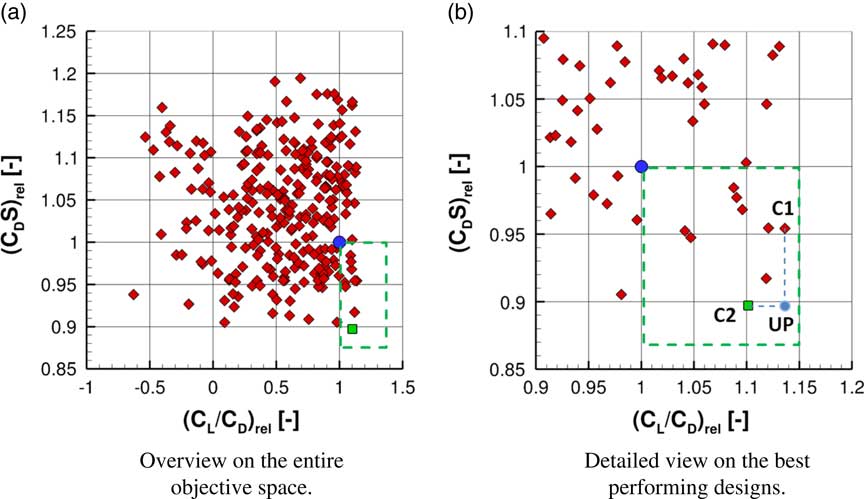
Figure 9. Objective space showing the evaluated designs from the multi-objective design optimisation.
Table 1 Comparison of the objective functions for the designs C1 and C2
Connecting the designs C1 and C2 leads to the utopia point UP for the current set of results. This point represents a theoretical design that combines the best of both objective functions. However, this point cannot be reached, because there is always a trade-off between the concurring objective functions. The distance between UP and any other design is taken into account to find a geometry, which offers a good compromise between both objective functions. The geometry with the smallest distance to UP is given by candidate C2, which is marked by a green symbol in Fig. 9. Moreover, this design is investigated in more detail and compared to the baseline geometry.
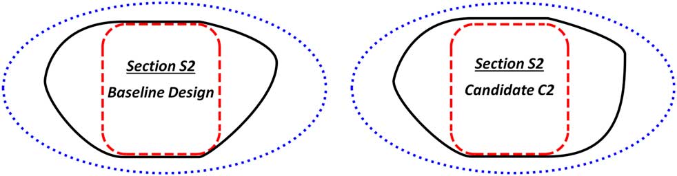
In order to exemplarily show the difference between the baseline geometry and the selected design C2, the chordwise pressure distribution is determined at the second radial blade-sleeve section S2. This section was chosen, because only minor interference effects with a large flow separation originating from the transition region between the full-fairing beanie and the BSF are present. The sectional shapes of the baseline design and candidate C2 are depicted in Fig. 10. Additionally, the design constraints, which were applied during the 2D design optimisation, are shown by red and blue lines. It can be observed that both designs are close to the minimum permissible design space.

Figure 10. Comparison between the sectional shapes of the baseline design and candidate C2 at the radial position S2. Red line: minimum permissible design space; blue line: maximum permissible design space.
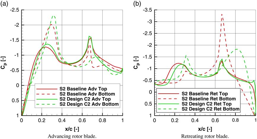
Figure 11 shows the chordwise pressure distribution C p(x/c) for the selected candidate C2 in comparison to the baseline design. The data were extracted from the second radial section S2. The results for the advancing RB are shown in Fig. 11(a) and for the retreating RB they are given in Fig. 11(b). The pressure distribution in Fig. 11(b) is mirrored, because reversed flow is present for the retreating blade. Regarding the pressure distribution on the upper surface of the BSF, which is represented by solid lines in both figures, no big differences can be observed. This is caused by the fact that the contour on the upper surface is quite similar for both designs. Hence, the same suction peak can be observed at x/c=0.65 for the advancing and the retreating RB, which is related to a strong curvature in the geometry. Concerning the bottom surface of the baseline design in Fig. 11(a), a pressure drop can be identified at 70% of the chord-length, which is related to a region of separated flow. The onset of flow separation is triggered by a strong curvature at x/c = 0.7. Furthermore, the smoothed contour of the optimised design C2 leads to a delayed flow separation within this region. Considering the retreating blade case in Fig. 11(b), a significant suction peak can be seen on the lower surface of the baseline design. In comparison to this, moderate pressure levels are obtained for candidate C2.

Figure 11. Comparison of the chordwise pressure distribution between the baseline design and the selected candidate C2 at section S2.
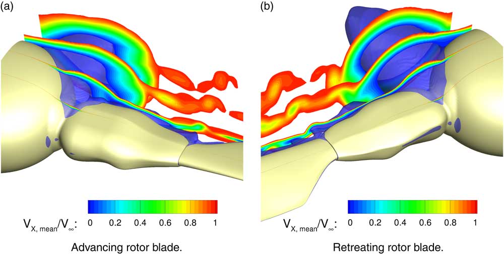
6.3 Flow field visualisation and 3D effects
At first, a general view on the prevailing flow field and the occurring flow phenomena is given. For this purpose, the simulation results of the baseline design are shown, which are representative for candidate C2 as well. The flow field is visualised by means of the averaged, axial flow velocity V
X, mean, which is normalised by the free-stream velocity V
∞. Figure 12 shows four slices in chordwise direction, which are located within a range of 0.5≤x/c≤1.5. Moreover, the results for the advancing and the retreating RB are illustrated in Fig. 12(a) and (b). The cut-off values for the contour plots are set according to
 $$(V_{{X,{\rm mean}}} \,/\,V_{\infty} )_{{{\rm min}}} {\equals}0$$
and
$$(V_{{X,{\rm mean}}} \,/\,V_{\infty} )_{{{\rm min}}} {\equals}0$$
and
 $$(V_{{X,{\rm mean}}} \,/\,V_{\infty} )_{{{\rm max}}} {\equals}1$$
. Additionally, an iso-surface is drawn at
$$(V_{{X,{\rm mean}}} \,/\,V_{\infty} )_{{{\rm max}}} {\equals}1$$
. Additionally, an iso-surface is drawn at
 $$V_{{X,{\rm mean}}} \,/\,V_{\infty} {\equals}0$$
for both cases. By means of this iso-surface, a large region of separated flow can be identified, which features reversed flow inside. The onset of flow separation is located in the transition region between the BSF and the full-fairing beanie, at approximately half of the chord length. Furthermore, the first blade-sleeve section S1 is influenced by this flow separation and reduced pressure levels are obtained compared to the two-dimensional simulation results. Moreover, the flow separation is larger for the retreating blade case, which can be seen in Fig. 12(b). Starting from a spanwise position of y/l
y
=0.5, almost undisturbed wake flow fields can be observed.
$$V_{{X,{\rm mean}}} \,/\,V_{\infty} {\equals}0$$
for both cases. By means of this iso-surface, a large region of separated flow can be identified, which features reversed flow inside. The onset of flow separation is located in the transition region between the BSF and the full-fairing beanie, at approximately half of the chord length. Furthermore, the first blade-sleeve section S1 is influenced by this flow separation and reduced pressure levels are obtained compared to the two-dimensional simulation results. Moreover, the flow separation is larger for the retreating blade case, which can be seen in Fig. 12(b). Starting from a spanwise position of y/l
y
=0.5, almost undisturbed wake flow fields can be observed.

Figure 12. Baseline fairing: normalised axial flow velocity V
X, mean/V
∞
shown at four evenly distributed x-slices within the region
 $$0.5\leq x\,/\,c\leq 1.5$$
.
$$0.5\leq x\,/\,c\leq 1.5$$
.
Furthermore, y-slices showing the averaged and normalised axial flow velocity are depicted in Fig. 13. These slices are located at the radial positions of the four supporting aerofoils (S1–S4). In comparison to the wake flow field of section S1, the region of reduced axial flow velocity is much smaller for the remaining sections S2–S4. In Fig. 13(b), the results for the retreating RB are shown. Concerning section S2, it can be observed that the flow separates earlier on the bottom surface, which leads to a flow deflection in downward direction. Additionally, the velocity deficit is more pronounced for the sections S1 and S2 compared to the advancing blade case in Fig. 13(a).
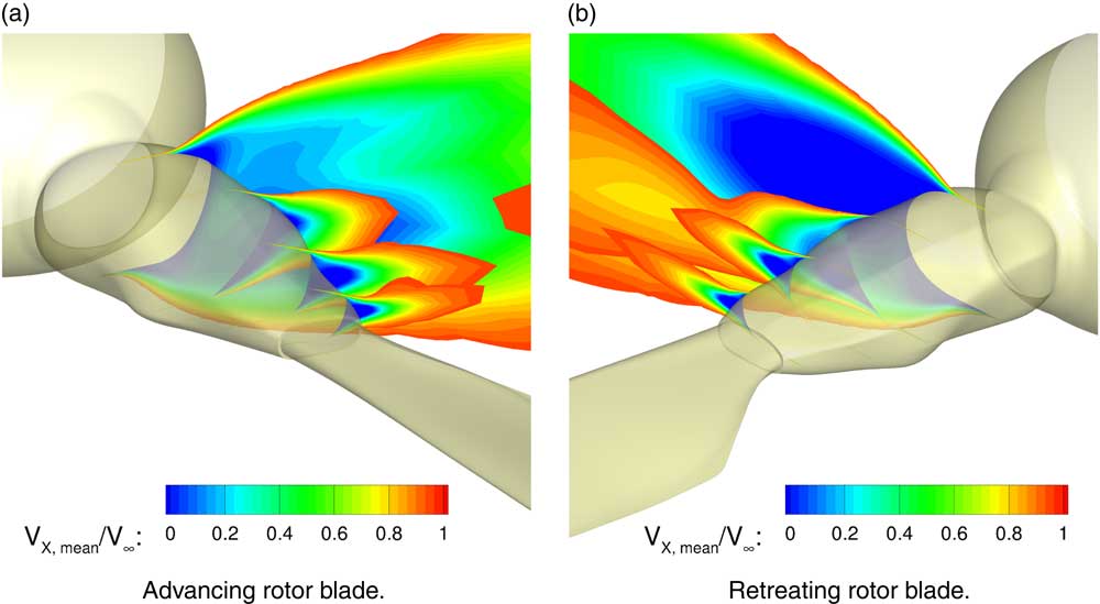
Figure 13. Baseline fairing: normalised axial flow velocity V X, mean/V ∞ shown at the four blade-sleeve sections S1–S4.
In order to determine the influence of the 3D effects, the results from the preliminary aerofoil optimisation are compared to the results from the 3D flow simulations. For this purpose, the chordwise pressure distributions are considered for the sections S1 and S3, which can be seen in Fig. 14. Regarding section S1, a large discrepancy between the aerofoil pressure distribution and the 3D result is present.
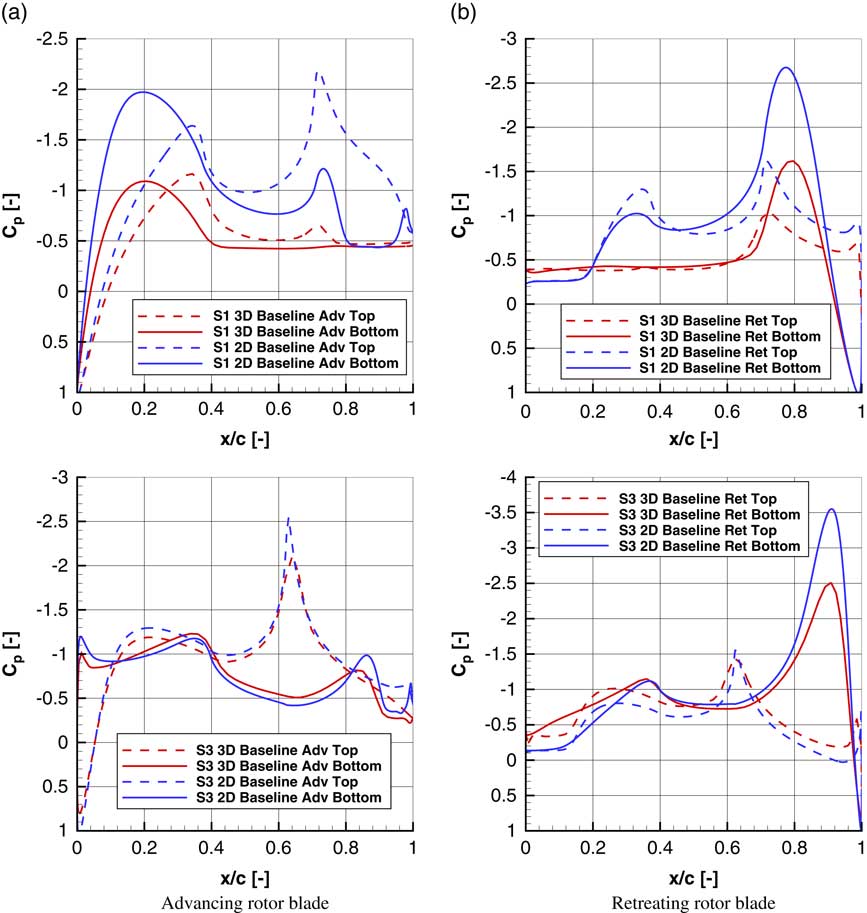
Figure 14. Comparison of the 2D and the 3D simulation results considering the pressure distribution C p(x/c) at the sections S1 and S3.
The flow field in this region is dominated by the flow separation between the BSF and the full-fairing beanie, which strongly influences the pressure distribution at this spanwise location. Hence, almost constant pressure is obtained over 60% of the chord length for the advancing as well as the retreating blade case. Regarding the pressure distributions of section S3, good agreement between the 2D and 3D results can be observed for both cases. However, a significant difference can be identified in the front region of the bottom surface for the retreating blade case, which is depicted in Fig. 14(b). Nevertheless, the present investigations show that a preliminary, two-dimensional design optimisation is reasonable for such an optimisation task. Furthermore, a sound database of aerofoils is available for the 3D design optimisation, which significantly reduces the number of required design variables.
Figure 15 shows the spanwise pressure distribution C
p(y/l
y
) for the baseline design as well as candidate C2. The results are derived from the centre of the fairing (x/c=0.5). The station y/l
y
=0 corresponds to the most inboard part of the BSF and y/l
y
=1 represents the transition to the rotor-blade. Furthermore, the results for the advancing RB are depicted in Fig. 15(a). Between 45% and 75% of the fairing length, an almost constant pressure gradient can observed for the upper surface of both designs. Moreover, the largest pressure difference between the upper and the lower surface is located at approximately 80% of the fairing length and design C2 reveals a bigger pressure difference than the baseline design on almost the entire length of the fairing. Furthermore, a significant pressure difference can be seen in the region 0.5≤y/l
y
 $$\, \leq 1$$
. Hence, the largest lift contribution is provided by this part of the BSF. Regarding the retreating blade case, which is shown in Fig. 15(b), lower pressure differences between the upper and the lower surface are obtained for both geometries. Additionally, the pressure gradient on the upper surface is reduced compared to the advancing blade case. At y/l
y
=0, almost the same pressure levels can be found for both cases. Further, design C2 provides a larger pressure difference between the upper and the lower surface in Fig. 15(b).
$$\, \leq 1$$
. Hence, the largest lift contribution is provided by this part of the BSF. Regarding the retreating blade case, which is shown in Fig. 15(b), lower pressure differences between the upper and the lower surface are obtained for both geometries. Additionally, the pressure gradient on the upper surface is reduced compared to the advancing blade case. At y/l
y
=0, almost the same pressure levels can be found for both cases. Further, design C2 provides a larger pressure difference between the upper and the lower surface in Fig. 15(b).
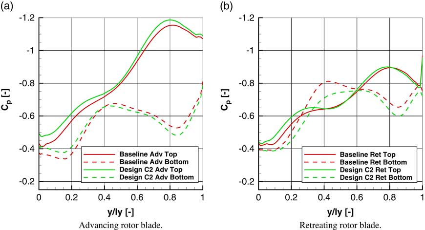
Figure 15. Spanwise pressure distribution C p(y/l y ) at the centre of the fairing (x/c=0.5) for the baseline design and candidate C2.
7.0 CONCLUSION
Within the present publication, the 3D aerodynamic design optimisation of the RACER BSF is described and first results of the ongoing optimisation process are shown. An isolated rotor head featuring a full-fairing beanie, a BSF and a truncated RB is examined. Furthermore, the parameterisation of the BSF is realised by four supporting aerofoils, which were aerodynamically optimised during previous work in the FURADO project. For each blade-sleeve section, 12 of the best performing aerofoils from the two-dimensional design optimisation were selected yielding the design variables for the present optimisation problem. The shape of the BSF is modified by replacing the supporting aerofoils. The applied objective functions are represented by the maximisation of the lift-to-drag ratio for the advancing RB (C L/C D) and the minimisation of drag (C D S) for the retreating RB. The optimisation is conducted by means of a multi-objective genetic algorithm and 334 designs have been evaluated so far. In order to be able to measure the performance improvement for a given design, a baseline candidate is generated for comparison. This baseline geometry is composed out of aerofoils, which yield the best compromise regarding both objective functions from the two-dimensional design optimisation. Additionally, the objective space is evaluated and a detailed view on the best performing geometries is given. In comparison to the baseline design, a maximum increase of (Δ C L/Δ C D)rel=13.6% was observed for the advancing blade case (design C1) and a reduction of (ΔCDS)rel=10.3% could be achieved for the retreating blade case (design C2). Moreover, design C2 represents the best compromise for both objective functions and it was selected to be investigated in more detail. For this purpose, the sectional shape as well as the chordwise pressure distribution of the second blade-sleeve section (S2) are compared to the baseline design. Additionally, the spanwise pressure distribution is examined at x/c=0.5 for both designs. Furthermore, a description of the flow field is given for the baseline geometry, which is representative for candidate C2 as well. Therefore, the averaged and normalised axial flow velocity is examined in four chordwise and spanwise slices. In order to determine any 3D effects, a comparison of the 2D and 3D simulation results is performed. Therefore, the sectional pressure distributions are derived for the first and the third blade-sleeve section (S1 and S3) of the baseline design.
ACKNOWLEDGEMENTS
The authors would like to thank the European Union for the funding of the FURADO research project within the framework of Clean Sky 2 under the grant agreement number 685636. Further, the fruitful collaboration and valuable support of the project partner Airbus Helicopters is highly acknowledged. Special thanks are addressed to ANSYS and the DLR for providing the flow simulation software. The authors gratefully acknowledge the Gauss Centre for Supercomputing e.V. (www.gauss-centre.eu) for funding this project by providing computing time on the GCS Supercomputer SuperMUC at Leibniz Supercomputing Centre (www.lrz.de).