NOMENCLATURE
- Z
blade number
- D
diameter of propeller disk, m
- d
spacing between the forward propeller and rear propellers, m
- Xf
axial distance ratio
- R
radius of propeller, m
- r
radius to the blade element, m
- c
chord length, m
- V a
axial inflow velocity, m/s
- V t
tangential inflow velocity, m/s
- N
rotation speed (per minute), r/min
- n
rotation speed (per second), r/s
- ω
angular rotation speed, rad/s
- CL
lift coefficient
- CD
drag coefficient
- Re
Reynolds number
- Ma
Mach number
- Γ
circulation
 $u_{a}^{*} $
axial-induced velocity, m/s
- $u_{t}^{*} $
tangential-induced velocity, m/s
- q
torque ratio, (Q 2/Q 1)
- λT
Lagrange multipliers for thrust
- λQ
Lagrange multipliers for torque
- ρ
air density, kg/m 3
- μ
dynamic viscosity, kg/(m ⋅ s)
- JS
advance ratio
- T
thrust of propeller, N
- Q
torque of propeller, N ⋅ m
- KT
thrust coefficient
- KQ
torque coefficient
- η
propeller efficiency, %
- $V_{a_{j} } $
axial inflow velocity
- $V_{t_{j} } $
tangential inflow velocity
- $u_{a_{j,\kern1pt j} }^{*} $
axial self-induced velocity on component j
- $u_{a_{j,k} }^{*} $
interaction-induced velocity on component j
- $u_{t_{j,\kern1pt j} }^{*} $
tangential self-induced velocity on component j
- $u_{t_{j,k} }^{*} $
interaction-induced velocity on component j
- $V_{j}^{*} $
resultant velocity on component j
- βj
inflow angle
- $\beta _{i_{j} } $
aerodynamic pitch angle
- αj
angle-of-attack
- θj
pitch angle of the aerofoil
- Tj
thrust force of the aerofoil
- Dj
tangential force of the aerofoil
- $F_{v_{j} } $
inviscid lift force
- $F_{i_{j} } $
viscous force
- Fj
resultant force
- j(n)
the nth control point on propeller j
- $u_{a_{j(n)} }^{*} $
axial-induced velocity induced by the individual horseshoe vortices
- $u_{t_{j(n)} }^{*} $
tangential-induced velocity induced by the individual horseshoe vortices
- $\overline{u}_{a_{j,k} }^{*} \left(n,m\right)$
axial velocity-induced factors at the nth control point of propeller j by horseshoe vortex of unit strength at the mth control point of propeller k
- $\overline{u}_{t_{j,k} }^{*} \left(n,m\right)$
tangential velocity-induced factors at the nth control point of propeller j by horseshoe vortex of unit strength at the mth control point of propeller k
- Γk (m)
circulation at the mth control point of propeller k
- (L / D)max
maximum lift-drag ratio
- ca
local air velocity.


Subscript
- j
the number of propellers (j = 1, j = 2 represents the forward and rear propeller, respectively)
- I
inviscid terms
- V
viscous terms
1.0 INTRODUCTION
In recent years, the high-altitude airships (HAAs) have received widespread attention in the aerospace sciences. The long endurance, low energy consumption and high security make HAAs attractive both in the military and civilian areas(Reference Jamison, Sommer and Porche1,Reference Colozza2) . The above features rely on a high-efficiency propulsion system. Until now, the propeller propulsion systems have been widely used in HAAs(Reference Liu, Duan, Ma and Ma3).
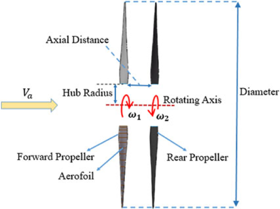
HAAs usually fly at about 20–30 km, where the environment is much different from that of low altitude. Therefore, the propeller operates under much lower air density, resulting in a low Reynolds number. Besides, the advance velocity is extremely low (about 10–30m/s). The above two factors make it difficult to achieve the same efficiency level as conventional propellers operating at relatively low altitude(Reference Liu, Tang, Chen and Guo4). Therefore, improving the propeller efficiency as much as possible has become a key problem(Reference Xu, Song, Yang and Zhang5). Based on conventional single propeller configurations, techniques such as co-flow jet flow control(Reference Zha, Carroll, Paxton and Conley6), plasma(Reference Cheng, Che and Nie7) and proplet(Reference Xu, Song and Yang8) techniques have been adopted to improve the propeller efficiency. However, the effects were found to be limited. Therefore, the concept of the contra-rotating propeller (CRP) was proposed for HAAs(Reference Tang, Liu, Chen and Guo9), which consists of two coaxial propellers positioned a short distance apart and rotating in opposite directions. Fig. 1 shows the simplified configuration of high-altitude contra-rotating propellers.

Figure 1. Simplified configuration of high-altitude contra-rotating propellers.
Many investigations on CRPs have been conducted in the last several decades, but mainly focused on the application on the vessel or airplane. Higher efficiency of CRPs over single propellers at low altitude has been validated(Reference Biermann and Gray10,Reference Paik, Hwang, Jung, Lee and Lee11) , mainly due to the recovery of the rotational energy losses originating from the forward propeller by the counter-rotating rear propeller(Reference Xin, Ding and Tang12). For example, wind tunnel tests conducted by Biermann and Hartman(Reference Biermann and Hartman13) showed that the contra-rotating propeller achieved higher power absorption and efficiency than a single propeller. McHugh and Pepper(Reference McHugh and Pepper14) found that the aerodynamically improved airfoil designs highly affect the performance of CRPs. But few of the above studies aimed at the applications at the operating conditions of low Reynolds number and small advance ratio. Recently, Tang et al. carried out wind tunnel tests for a stratospheric airship CRP scaling model (diameter of 0.75 m) and showed that the counter-rotating propeller would be a wise option applied on stratospheric airships(Reference Tang, Liu, Chen and Guo9).
Similar to the single propeller design, the CRP design also aims to obtain the best parameter adjustments for the front and rear propellers. The parameters of a CRP include blade number, diameter, individual rotation speed for both propellers, axial distance, radial variation of cross-sectional profile shape, pitch angle, and chord length. However, due to the interference of the front and rear propellers, the maximum individual efficiency of the front or rear propeller does not necessarily mean the most desired CRP total efficiency. Therefore, the design of CRPs requires the coupling of optimization of the front and rear propellers.
Over the years, the Vortex Lattice Lifting Line Method (VLM) has been a commonly used method of designing propellers. This method gives a good prediction of the air propeller efficiency with large blade aspect ratios(Reference Coney15–Reference Epps and Kimball17). The first lifting line method for CRP was proposed by Lerbs(Reference Lerbs18). His approach was an extension of the single propeller lifting line considering the interaction velocities induced by each propeller on the other. The blade numbers for the forward and the rear propellers were assumed the same. Lerb’s theory was then developed by Morgan and Wrench(Reference Morgan19,Reference Morgan and Wrench20) with the extension of any combination of blade numbers and derivation of accurate equations to compute the interactive induced velocities. They designed the CRPs by coupling two single propellers’ code in an iterative way,which was actually an ‘uncoupled’ method. Kerwin et al.(Reference Kerwin, Coney and Hsin21) proposed a ‘coupled’ method, considering the CRP as an integrated propulsive unit and giving an iterative procedure to calculate the optimum circulation distribution at each propeller. The generalized numerical CRP variational optimizer for the ‘uncoupled’ and ‘coupled’ method was implemented by Laskos(Reference Laskos22). Kravitz established an off-design analysis procedure to predict the performance for a given CRP, which was an extension of the single propeller off design analysis proposed by Epps(Reference Epps23).
However, the above methods did not consider the effects of the Reynolds number and Mach number on aerofoil at different radial locations, which significantly affect the performance of high-altitude CRPs. Besides, the chord length distributions were assumed the same for both propellers and were not part of the propeller circulation optimization process. However, as shown in the single propeller optimization study conducted by Zheng et al.(Reference Zheng, Wang, Cheng and Han24), by taking into account the viscous effects of the chord length and optimizing the chord length distribution, higher efficiency of the single propeller can be achieved. Therefore, there is a need to introduce the individual chord length distributions for each propeller as optimized variables in the coupling optimization process for the high-altitude CRPs. Furthermore, as there is interference between the front and rear propellers, which is different from that of the high-altitude single propeller, the investigations on how the parameters such as blade numbers, diameter, rotation speeds, axial distance and torque ratio affect the optimum CRP efficiency need to be conducted as well.
The aim of this study is to develop an improved efficient variational optimization method for high-altitude CRPs based on the Kerwin’s CRP optimizer(Reference Kerwin, Coney and Hsin21), which can consider the chord length distribution optimization and effects of the Reynolds number and the Mach number of aerofoil and investigate the effects of parameters on the optimum efficiency of high-altitude CRPs in detail. The desired circulation distribution, chord and pitch distribution are obtained under the maximum lift-to-drag ratio of aerofoils. The aerofoil aerodynamics data used in the iterative optimization process, such as lift, drag coefficient and lift-to-ratio, are obtained by interpolating a CFD database, which was established by numerical simulations for the different Reynolds number, Mach number and angles-of-attack. Therefore, the effects of the Reynolds number and the Mach number can be considered. The improved method is validated by using the three-dimensional steady Reynolds-averaged Navier-Stokes (RANS) solver and moving reference frames (MRF) technique. Using the improved approach, parametric studies are conducted in detail to illustrate how the optimum efficiency of high-altitude CRPs is influenced by the parameters of blade numbers, diameter, rotation speeds, the axial distance and torque ratio.
The paper is organized as follows. First, the improved algorithms for the contra-rotating propeller optimizer will be described in Section 2.0. Then, in Section 3.0, the validations are conducted by comparing the present results with the CFD data. In Section 4.0, the effects of parameters on the optimum CRP efficiency are investigated in detail. Last, in Section 5.0, the conclusions will be drawn.
2.0 METHODOLOGY
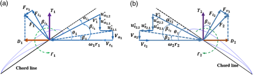
The velocity, angle and forces diagram of the blade aerofoil for both propellers are shown in Fig. 2. As the slipstream is assumed purely axial (no contraction of the incoming streamtube), the radial interaction velocity is set to zero.

Figure 2. Velocity, angle and forces diagram of the CRP blade aerofoil: (a) Forward propeller. (b) Rear propeller.
The total thrust T and torque Q of the CRP are:
 \begin{equation}T=\sum _{j=1}^{2}\left\{T_{j} \right\} =\sum _{j=1}^{2}\left\{T_{I_{j} } +T_{V_{j} } \right\}\end{equation}
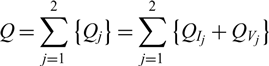 \begin{equation}Q=\sum _{j=1}^{2}\left\{Q_{j} \right\} =\sum _{j=1}^{2}\left\{Q_{I_{j} } +Q_{V_{j} } \right\}\end{equation}
where
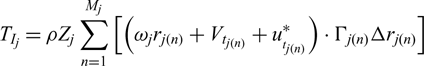 \begin{equation}T_{I_{j} } =\rho Z_{j} \sum _{n=1}^{M_{j} }\left[\left(\omega _{j} r_{j\left(n\right)} +V_{t_{j\left(n\right)} } +u_{_{t_{j\left(n\right)} } }^{*} \right)\cdot \Gamma _{j(n)} \Delta r_{j(n)} \right]\end{equation}
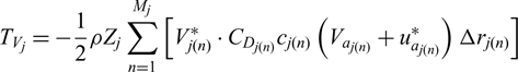 \begin{equation}T_{V_{j} } =-\frac{1}{2} \rho Z_{j} \sum _{n=1}^{M_{j} }\left[V_{j(n)}^{*} \cdot C_{D_{j(n)} } c_{j(n)} \left(V_{a_{j(n)} } +u_{a_{j(n)} }^{*} \right)\Delta r_{j(n)} \right]\end{equation}
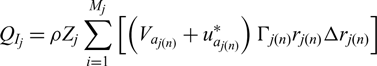 \begin{equation}Q_{I_{j} } =\rho Z_{j} \sum _{i=1}^{M_{j} }\left[\left(V_{a_{j(n)} } +u_{a_{j(n)} }^{*} \right)\Gamma _{j(n)} r_{j(n)} \Delta r_{j(n)} \right]\end{equation}
 \begin{equation}Q_{V_{j} } =\frac{1}{2} \rho Z_{j} \sum _{i=1}^{M_{j} }\left[V_{j(n)}^{*} C_{D_{j(n)} } c_{j(n)} \left(\omega _{j} r_{j(n)} +V_{t_{j(n)} } +u_{t_{j(n)} }^{*} \right)r_{j(n)} \Delta r_{j(n)} \right]\end{equation}
And  $u_{a_{j(n)} }^{*} $ and
  $u_{t_{j(n)} }^{*} $ can be written as:
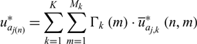 \begin{equation}u_{a_{j(n)} }^{*} =\sum _{k=1}^{K}\sum _{m=1}^{M_{k} }\Gamma _{k} \left(m\right)\cdot \overline{u}_{a_{j,k} }^{*} \left(n,m\right)\end{equation}
 \begin{equation}u_{t_{j\left(n\right)} }^{*} =\sum _{k=1}^{K}\sum _{m=1}^{M_{k} }\Gamma _{k} \left(m\right)\cdot \overline{u}_{t_{j,k} }^{*} \left(n,m\right)\end{equation}
where  $\overline{u}_{a_{j,k} }^{*} \left(n,m\right)$ and
  $\overline{u}_{t_{j,k} }^{*} \left(n,m\right)$ can be calculated by the wake alignment model(Reference Epps and Kimball17).
Therefore, the propulsive efficiency of CRP can be written as:
 \begin{equation}\eta =\frac{\sum\limits_{j=1}^{2}\left(T_{j} V_{a} \right) }{\sum\limits_{j=1}^{2}\left(Q_{j} \omega _{j} \right) }\end{equation}
In this paper, V a is assumed to be equal to the advance speed of the airship V s.
For a given total thrust T r and the specific torque ratio  $q=\frac{Q_{2} }{Q_{1} } $ to achieve the maximum efficiency, an auxiliary function H is formed by introducing two Lagrange multipliers λT, λQ (Reference Kerwin, Coney and Hsin21):
 \begin{equation}H=\left(\omega _{1} Q_{1} +\omega _{2} Q_{2} \right)+\lambda _{T} \left(T_{1} + T_{2} -T_{r} \right)+\lambda _{Q} \left(qQ_{1} -Q_{2} \right)\end{equation}
If T 1 + T 2 = T r, qQ 1 = Q 2, then the minimal H is obtained as H min = (ω 1Q 1 + ω 2Q 2), and the derivatives of H with respect to the unknown circulation values and Lagrange multipliers are set to be zero,
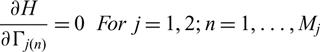 \begin{equation}\frac{\partial H}{\partial \Gamma _{j(n)} } =0\; \; \; For\; \; j=1,2;n=1,\ldots,M_{j}\end{equation}
 \begin{equation}\frac{\partial H}{\partial \lambda _{T} } =0\end{equation}
 \begin{equation}\frac{\partial H}{\partial \lambda _{Q} } =0\end{equation}
Then, a system of M 1 + M 2 + 2 nonlinear equations with the same number of unknown variables can be obtained. This nonlinear problem can be linearized by freezing parameters  $u_{a_{j} }^{*} , u_{t_{j} }^{*} ,\overline{u}_{a_{j,k} }^{*} ,\overline{u}_{t_{j,k} }^{*} ,V_{j}^{*} ,\lambda _{T}, $ and λQ and iteratively solved by updating them at each iteration. And then the circulation distribution can be obtained. More details can be found in Kerwin(Reference Kerwin, Coney and Hsin21).
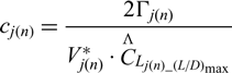
Using the convergent optimum circulation Γj(n) and resultant velocity.  $V_{j(n)}^{*} $, and assuming all aerofoil sections working at the maximum lift-drag ratio (L/D) max. cj(n) can be obtained as:
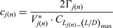 \begin{equation}c_{j\left(n\right)} =\frac{2\Gamma _{j(n)} }{V_{j(n)}^{*} \cdot C_{L_{j\left(n\right)} \_ \left({L\mathord{\left/ {\vphantom {L D}} \right.} D} \right)_{\max } } }\end{equation}
 Substituting Equation (14) and the  $C_{D_{j\left(n\right)} \_ \left({L\mathord{\left/ {\vphantom {L D}} \right. } D} \right)_{\max } } $ into Equations (4) and (6),
  $T_{V_{j} } $ and
  $Q_{V_{j} } $ can be rewritten as:
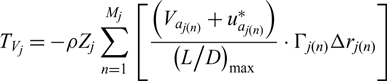 \begin{equation}T_{V_{j} } =-\rho Z_{j} \sum _{n=1}^{M_{j} }\left[\frac{\left(V_{a_{j(n)} } +u_{a_{j(n)} }^{*} \right)}{\left({L\mathord{\left/ {\vphantom {L D}} \right.} D} \right)_{\max } } \cdot \Gamma _{j(n)} \Delta r_{j(n)} \right]\end{equation}
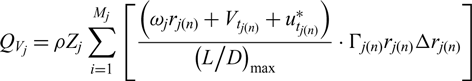 \begin{equation}Q_{V_{j} } =\rho Z_{j} \sum _{i=1}^{M_{j} }\left[\frac{\left(\omega _{j} r_{j(n)} +V_{t_{j(n)} } +u_{t_{j(n)} }^{*} \right)}{\left({L\mathord{\left/ {\vphantom {L D}} \right.} D} \right)_{\max } } \cdot \Gamma _{j(n)} r_{j(n)} \Delta r_{j(n)} \right]\end{equation}
 Now the systems can be linearized by freezing parameters  $u_{a_{j} }^{*} ,u_{t}^{*} ,\overline{u}_{a_{j} }^{*} ,\overline{u}_{t_{j} }^{*}, C_{L_{j\left(n\right) \_ \left({L\mathord{\left/ {\vphantom {L D}} \right.} D} \right)_{\max } }}$,
  $C_{D_{j\left(n\right)\_ \left({L\mathord{\left/ {\vphantom {L D}} \right. } D} \right)_{\max } } } ,({L\mathord{\left/ {\vphantom {L D}} \right. } D} )_{\max } , \lambda _{T} $ and λQ.
cj(n) should be calculated before updating (L / D)max,
 \begin{equation}c_{j\left(n\right)} =\frac{2\Gamma _{j(n)} }{V_{j(n)}^{*} \cdot \mathop{C}\limits^{\Lambda } \kern-2.2pt{}_{L_{j\left(n\right)\_ \left({L\mathord{\left/ {\vphantom {L D}} \right. } D} \right)_{\max } } } }\end{equation}
where 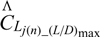 $\mathop{C}\limits^{\Lambda } \kern-2.2pt{}_{L_{j\left(n\right)\_ \left({L\mathord{\left/ {\vphantom {L D}} \right. } D} \right)_{\max } } } $ is a frozen value and
  $V_{j(n)}^{*} $ is
 \begin{equation}V_{j(n)}^{*} =\sqrt{\left(V_{a_{j(n)} } +u_{a_{j(n)} }^{*} \right)^{2} +\left(V_{t_{j(n)} } +\omega _{j} r_{j(n)} +u_{t_{j(n)} }^{*} \right)^{2} }\end{equation}
 The Reynolds number Rej(n) and Mach number Maj(n) of the aerofoil are respectively obtained by using cj(n) and  $V_{j(n)}^{*} $,
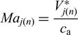 \begin{equation}Ma_{j(n)} =\frac{V_{j(n)}^{*} }{c_{{\rm a}} }\end{equation}
 \begin{equation}Re_{j(n)} =\frac{\rho c_{j(n)} V_{j(n)}^{*} }{\mu }\end{equation}
 By using Rej(n) and Maj(n), we can obtain the new (L/D)max and the corresponding  $C_{L_{j\left(n\right)} \_ ({L\mathord{\left/ {\vphantom {L D}} \right. } D} )_{\max } } ,C_{D_{j\left(n\right)\_ ({L\mathord{\left/ {\vphantom {L D}} \right. } D} )_{\max } } } $ and
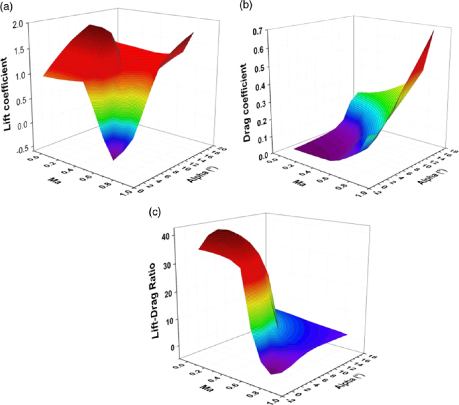
  $\alpha _{j(n)\_ ({L\mathord{\left/ {\vphantom {L D}} \right. } D} )_{\max } } $ by automatically interpolating the CFD database(Reference Zheng, Wang, Cheng and Han24). The low-Reynolds-number and high-lift airfoil S1223(Reference Selig and Guglielmo25,Reference Ma and Liu26) is chosen and its aerodynamics is simulated by software FLUENT in the ranges of Re = 3, 000 ∼ 2.0 × 10⁷, Ma = 0.05 ∼ 0.9 and α = 0° ∼ 16°. Fig. 3 shows the contour of lift, drag and lift-drag ratio variations with Mach numbers and angles of attack at Re = 60, 000.

Figure 3. (a) The lift coefficient, (b) drag coefficient, (c) lift-drag ratio with variation with Mach numbers and angles of attack (Re = 60, 000).
As is shown in Fig. 2,  $\beta _{i_{j(n)} } $ can be written as,
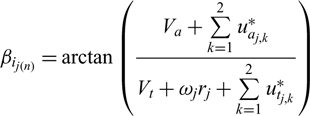 \begin{equation}\beta _{i_{j\left(n\right)} } =\arctan \left(\frac{V_{a} +\sum\limits_{k=1}^{2}u_{a_{j,k} }^{*} }{V_{t} +\omega _{j} r_{j} +\sum\limits_{k=1}^{2}u_{t_{j,k} }^{*} } \right)\end{equation}
And the pitch angle θj(n) is
 \begin{equation}\theta _{j(n)} =\alpha _{j(n)\_ \left({L\mathord{\left/ {\vphantom {L D}} \right. } D} \right)_{\max } } +\beta _{i_{j(n)} }\end{equation}
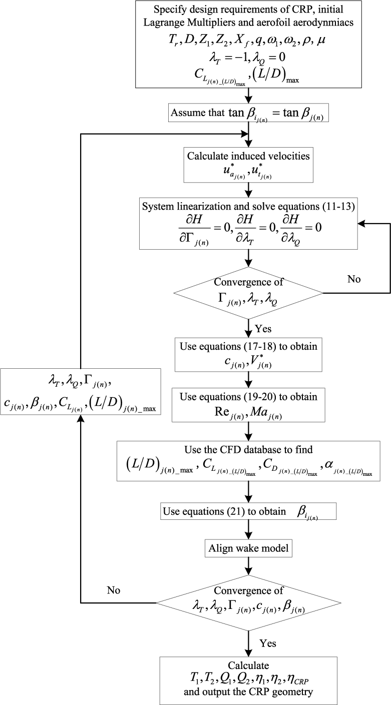
 Finally,  $\lambda _{Q} ,\lambda _{T} ,\Gamma _{j(n)} ,\beta _{i_{j(n)} } $ and cj(n) can be iteratively optimized until all variables satisfy the prescribed convergence criterion. The framework of the present optimum design method for contra-rotating propellers is shown in Fig. 4.

Figure 4. The framework of the present optimum design method for contra-rotating propellers.
3.0 VALIDATIONS
To validate the present method, computational results of thrust, torque and efficiency are compared with the CFD results. The CRP is optimized by the present approach with the following design conditions:
Altitude: 20km
Air density: 0.0889 kg/m3
Advance speed: Vs = 20m/s
Required thrust: Tr = T1 + T 2 = 380N
Torque ratio:
$q=\frac{Q_{2} }{Q_{1} } =1$Propeller diameter: D = D 1 = D 2 = 5.5m
Rub diameter: 0.2D
Design advance ratio:
$J_{S_{1} } =J_{S_{2} } =0.545$

The Fluent steady RANS solver(27) is used to conduct the CFD simulations. The density-based solver is used to solve the control equations, with single precision and second order in space. The courant number is 5. The one-equation Spalart-Allmaras (S-A) turbulence model is adopted(Reference Spalart and AllMarchas28). The non-reflective boundary condition is set. The inlet velocity boundary condition and pressure far-field boundary condition are adopted for all simulations.
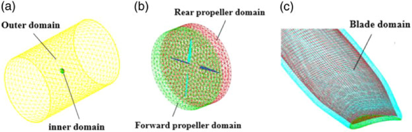
Fig. 5 shows the computational domains for simulating the flow field of contra-rotating propeller. The overall computational grid is generated with unstructured mesh and extends 20 times the radius of CRP (the cell number is 1.16 million). The mesh is divided into three parts: two inner regions for the forward propeller and the rear propeller and one outer region. The overlapping surface between different domains is defined as the interface. The boundary layer is generated and the value of Y+ (average) is about 10. The moving reference is used to define the rotation motion of the forward and rear propeller individually. The absolute rotation speeds of the two moving references are equal to the rotation speed of the two propellers, individually. The outer domain is set to be stationary.

Figure 5. Computational domains of contra-rotating propeller (a) overall domain, (b) inner propeller domain, (c) blade domain.
Note that as there is no standard model for the high-altitude contra-rotating propellers, the CFD results are used to estimate the precision of the present method. Therefore, the error mentioned below is relative to the CFD data, which is assumed to have small errors.
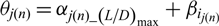
Fig. 6 shows the optimum chord and pitch angle distributions of CRP. It can be seen that both the optimum chord and pitch angle distributions of the forward propeller differ from that of the rear propeller.
Figure 6. The optimum chord (c/D) and pitch angle distribution of the optimum CRP.
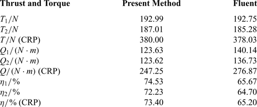
Table 1 shows the results optimized by the present method, which are compared with the numerical results simulated by Fluent based on the configuration of the optimum CRP. In the figure, we can see that the thrust, torque and efficiency match well with the CFD data, both for the individual front and rear propellers and CRP. The optimum CRP efficiency from the present method is about 8.2% higher than that of Fluent. Since the rear propeller operates in the accelerated slipstream of the front propeller, the effective attack angle of the rear propeller is decreased. As a result, the torque (Q 2) and efficiency (η 2) of rear propeller are somewhat lower than those of front one.
Table 1 Comparisons between the results optimized by the present method and Fluent

The comparisons of the propulsion performance under different advance ratios between the present method and Fluent are shown in Fig. 7. Thrust coefficients (KT), torque coefficients (KQ) and efficiency of CRP with variation of advance coefficients are given. KT and KQ are defined by
 \begin{equation}KT=\frac{T}{\rho n_{s}^{2} D^{4} }\end{equation}
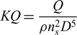 \begin{equation}KQ=\frac{Q}{\rho n_{s}^{2} D^{5} }\end{equation}
where ns is the rotation speed per second and D is the diameter of the CRP.
Figure 7. Comparisons of the performance under different advance ratio between the present method and CFD: (a) thrust coefficients, (b) torque coefficients, (c) efficiency of the CRP.
It can be seen in Fig. 7 that the predicted CRP performance from the present method correlates well with the Fluent. The calculated KT curve closely matches that obtained by the Fluent, except that it is slightly underestimated at the low advance coefficients (Js < 0.35). However, the calculated KQ data are somewhat lower than the CFD results. The present results of efficiency curve have the same trend with CFD, and the advance coefficient for the maximum efficiency closely matches the CFD results. Mainly due to the underprediction for torque coefficients, the calculated results of efficiency are generally higher than the CFD results. At the advance coefficient where the maximum efficiency is achieved, it is about only 6% higher than the CFD data. The validations show that the present method can be used to optimize and analyse the efficiency of high-altitude CRPs.
4.0 RESULTS AND DISCUSSIONS
As the optimum CRP efficiency depends on both propellers, parametric studies for CRP are not the same as for the single propeller. In this section, detailed parametric studies are conduced to illustrate how the optimum efficiency of high-altitude CRP is influenced by the variations of several propeller parameters, including blade number, propeller diameter, rotation speed, axial distance and torque ratio. The thrust required on a stratosphere airship is used as the design condition. The parameters of airship and thrust for each CRP propulsion system are shown in Table 2. The hub diameters for all simulations are assumed to be 0.1 D.
Table 2 Parameters of airship and thrust for each CRP propulsion system
4.1 Blade number
The first parametric study is to investigate the effects of blade number for each propeller. The axial distance ratio is  $X_{f} =\frac{d}{R} =0.3$, propeller diameter is D 1 = D 2 = 6m and torque ratio is
  $q=\frac{Q_{2} }{Q_{1} } =1$. The study is conducted for a range of propeller speeds, assuming both propellers rotate at the same speeds (N 1 = N 2).
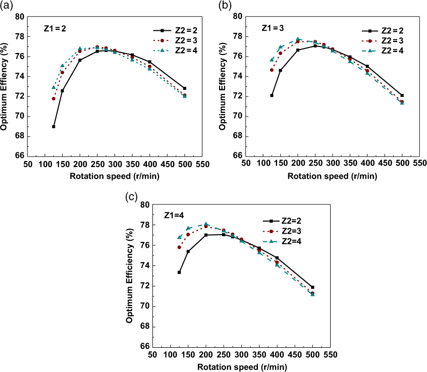
Fig. 8 shows the optimum efficiency for different blade numbers of the forward and rear propellers. As shown in the figure, for all combinations of Z 1 and Z 2, the optimum efficiency of the CRP first increases and then decreases with the increase of rotation speeds, with a maximal value at certain rotation speed. For a certain blade number of the forward propeller, the optimum efficiency first increases with the increase of the blade number of the rear propeller under relatively low rotation speeds (N < 300r/min). But then, with the increase of the rotation speed, higher optimum efficiency is found to be achieved by a lower Z 2. This is probably because at high rotation speeds, the blade-to-blade interaction becomes stronger with Z 2 increases; thus, the performance of CRPs deteriorates and the efficiency decreases.

Figure 8. Optimum efficiency of CRP for different blade numbers (a) Z 1 = 2, Z 2 = 2,3,4, (b) Z 1 = 3, Z 2 = 2,3,4, (c) Z 1 = 4, Z 2 = 2,3,4.
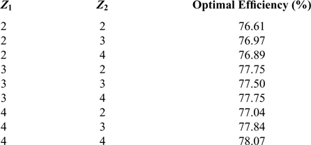
The most efficient CRP configurations with respect to the number of blades are summarized in Table 3. The combination of blade numbers Z 1 = 4, Z 2 = 4 achieves the highest efficiency of 78.07%, which is 1.46% higher than the configuration of Z 1 = Z 2 = 2. However, considering that more blades are required for the former configuration, the structure weights as well as manufacturing cost and difficulty will be higher. Therefore, a trade-off analysis on the choice of combinations of blade number needs to be conducted in the engineering design of the CRP propulsion system for high-altitude airships. In the following parametric studies, the configuration of Z 1 = Z 2 = 2 is chosen for all cases.
Table 3 The optimal efficiency for different combinations of front and rear propeller blade numbers

4.2 Diameter and rotation speed
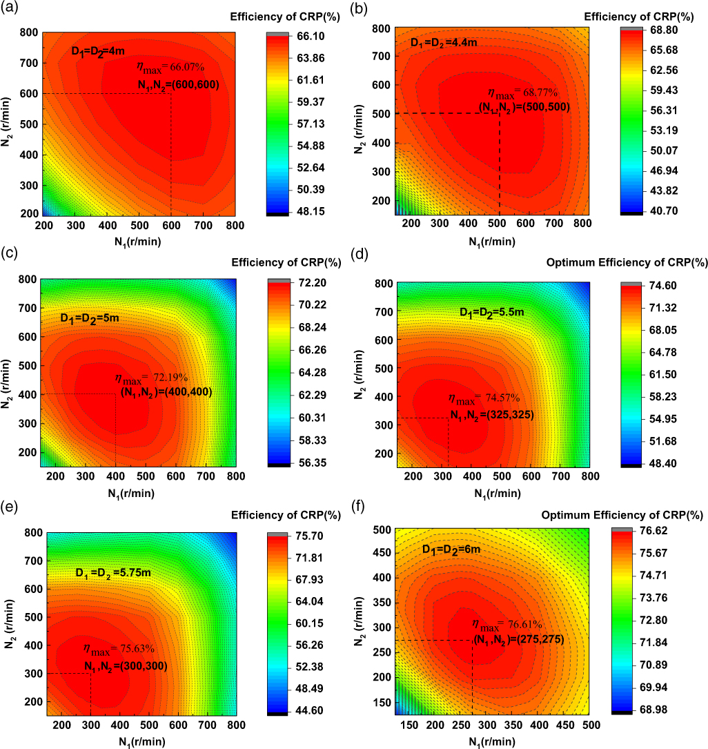
For the CRP propulsion system of the HAAs, the two propellers can be driven by two individual motors; thus, there is no requirement that the two propellers must rotate at the same speeds. In Section 4.1 the assumptions of diameters keeping unchanged and both propellers rotating at the same speed are adopted. In this section, however, there is no constraint for both propellers rotating at the same speed and diameter keeping constant, so the effects of different configurations will be analysed for a range of propeller speeds and diameters. Figure 8 shows the optimum efficiency of CRPs under different diameters, varying with rotation speeds of the front propeller and the rear propeller. The horizontal axis represents the forward propeller rotation speed (N 1), and the vertical axis represents the rear propeller rotation speed (N 2).
It can be seen in Fig. 9 that for each diameter, the optimum efficiency has a maximal value with the variation of N 1 and N 2. It can be seen that the optimum efficiency is highly affected by the diameter. The maximum efficiency generally increases with the increases of diameter. And it is interesting to see that even though there is no constraint that the forward and rear propellers rotate at the same rotation speeds, the maximum efficiency for each diameter is consistently achieved when both propellers are rotating at the same speed (N 1 = N 2). And the optimum rotation speeds decrease with the increases of diameter. The maximum efficiency of 76.61% is achieved at D = 6m, [N 1, N 2] = [275rpm, 275rpm]. Besides, it is observed that, at a certain diameter, the optimum efficiency is not significantly affected by the rotation speed difference of the two propellers. For example, when D = 6m and N 1 = 350rpm, the optimal efficiency 76.43% is achieved at N 2 = 250rpm, while the efficiency is 76.17% at N 2 = N 1 = 350rpm, which is only 0.26% lower than the optimal value. However, the difference of design rotation speeds between the forward and rear propellers indicates different design conditions for the development of driving motors, leading to the requirement of two different motors for a CRP propulsion system. Therefore, if the optimum design rotation speeds of the two propellers are found to be different (N 1 ≠ N 2), which makes the CRP system more expensive or complicated, we can probably design the two propellers rotating at the same rotation speeds without significantly decreasing the efficiency of CRP.

Figure 9. Optimum efficiency of CRP for different propeller diameter.
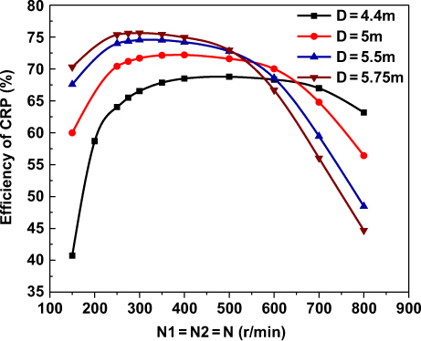
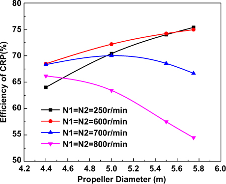
Fig. 10 shows the optimum efficiency of CRP for different propeller diameters, where both propellers are rotating at the same speeds. It can be seen that the optimum efficiency has a maximal value at a certain rotation speed. However, the maximal efficiency has no significant difference with that achieved at the neighbouring rotation speeds. Fig. 11 shows the optimum efficiency of CRP for different design rotation speeds. We can see that, under different design rotation speeds, the effects of the diameter on the optimum efficiency are not consistent. In the present design region of diameter, when N = 250rpm and N = 600rpm, the increase of diameter is totally beneficial to the optimum efficiency; when N = 700rpm, a maximal efficiency is obtained at D = 5m; and when N = 800rpm, the optimum efficiency decreases with the increases of diameter. Sometimes, high-altitude CRP propulsion systems are designed with limited available selections of driving motors whose optimal rotation speeds are certain. Under this prescribed design condition, the diameter of CRP needs to be suitably designed to achieve high efficiency.

Figure 10. Optimum efficiency of CRP for different propeller diameters.

Figure 11. Optimum efficiency of CRP for different design rotation speeds.
4.3 Axial distance
In the parametric analysis in the previous sections, the axial distance d = 0.3R  $(X_{f} =\frac{d}{R} =0.3)$ between the front and rear propellers were assumed for all optimization cases. This section will investigate the effects of different axial distances on the CRP optimum efficiency. The other parameters of the CRP used here are chosen based on the parametric studies in section 4.1 and section 4.2. (Z 1 = Z 2 = 2, D = 6m, N1 = N2 = 275rpm). Only the axial distance is allowed to vary with Xf ranging from 0.2 to 1.0. The optimum CRP efficiency varying with Xf is shown in Fig. 12. The geometric pitch ratio PD at r = 075R
 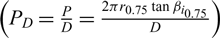 $\left(P_{D} =\frac{P}{D} =\frac{2\pi r_{0.7{\rm 5}} \tan \beta _{i_{0.7{\rm 5}} } }{D} \right)$ for both propellers is also given in the figure.
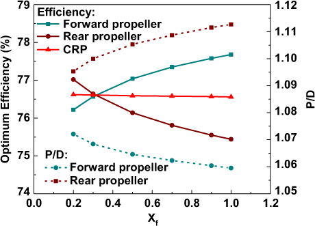
Figure 12. Optimum efficiency and pitch ratio variations with the axial distance between the front propeller and rear propeller.
In the figure, we can see that the axial distance has obvious effects on the individual efficiency of each propeller. The efficiency of the forward propeller increases with the increases of Xf, mainly because lower axial velocity is induced by the rear propeller, resulting in a lower required PD. Conversely, with the increases of Xf due to higher axial velocity induced by the forward propeller, the efficiency increases and the required P D decreases for the rear propeller. When Xf is relatively small (Xf < 0.3), the rear propeller efficiency is higher than that of forward propeller while it is contrary for higher Xf. However, as shown in the figure, the total optimum CRP efficiency is slightly affected by the variation of Xf.
4.4 Torque ratio
In previous sections, the prescribed torque for both propellers were assumed to be equal (torque ratio  $q=\frac{Q_{2} }{Q_{1} } {\rm =1}$). In this section, the effects of this parameter on the optimum efficiency will be investigated. The torque ratio is allowed to be changed from 0.5 to 2.0.
Fig. 13 shows the optimum efficiency of CRP for different torque ratios. As shown in the figure, it is interesting to find that the maximum efficiency is achieved when q = 1.0, even without the constraint of both propellers having the same torque. This is probably because when q = 1.0, the aerodynamic loads on both propellers are very close under the same rotation speed, and the tangential interaction induced velocity on the rear propeller induced by the forward propeller can exactly counteract its self-induced velocity. Therefore, the rear propeller can most efficiently recover the rotational energy losses originating from the forward propeller in this case. However, the efficiency has no significant difference under a different torque ratio. The maximum efficiency is about 76.61% when q = 1.0, which is 0.61% higher than the lowest value of 76.0% when q = 0.5. Considering that the maximum efficiency is achieved at same torque and rotation speeds for both propellers, it is beneficial to the design of a high-altitude CRP propulsion system, especially for reducing the complexity of motor design.
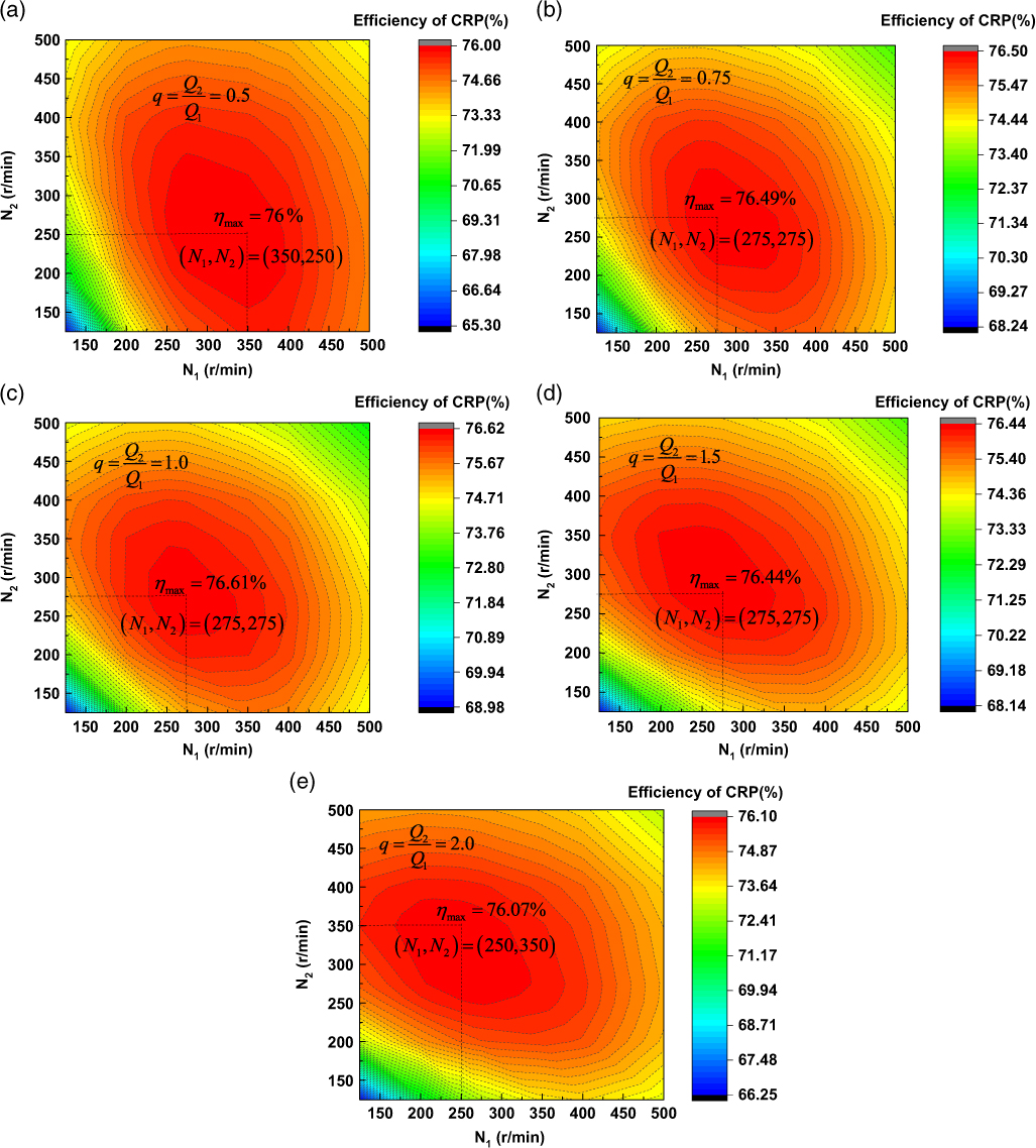
Figure 13. Optimum efficiency of CRP for different torque ratios.
The three-dimensional configuration of the contra-rotating propeller finally designed is shown in Fig. 14.
Figure 14. The three-dimensional configuration of the contra-rotating propeller finally designed.
5.0 CONCLUSIONS
The efficiency of high-altitude contra-rotating propellers will significantly affect the overall performance of stratosphere airship. An improved optimization algorithm based on the vortex lifting line method is established in designing the high-altitude CRPs. The chord length and pitch distributions for the forward and rear propeller are obtained by coupling optimization with considering the radial variation of Reynolds numbers and Mach numbers. The improved approach is validated by CFD method. The optimization results for a high-altitude CRP show a good agreement with CFD, indicating that the method can be used as an efficient tool to select the CRPs in the preliminary stage of stratosphere aircraft design. Besides, by conducting detailed parametric optimizations, the effects of rotation speeds, propeller diameter, blade number, axial distance and torque ratio on the optimum efficiency are illustrated in detail, which are helpful to the design of high-altitude CRPs. Assuming no constraint for the design rotation speeds, the diameter and blade numbers affect the optimum efficiency in a relatively high degree while the effects of axial distance and torque ratio is relatively lower. Some main conclusions include:
1. For a certain blade number of the forward propeller, the optimum efficiency first increases with the increase of the blade number of the rear propeller. But then, with the increase of the rotation speed, higher optimum efficiency is achieved by a lower blade number of the rear propeller. And a trade-off analysis on the choice of blade numbers for high-altitude CRPs needs to be conducted, considering the efficiency, structure weights, manufacturing cost and difficulty.
2. The diameter highly affects the optimum efficiency of CRPs. The maximum efficiency generally increases with the increases of the diameter. The maximum efficiency for each diameter is achieved when both propellers rotate at the same speed. Besides, under different design rotation speeds, the effects of the diameter on the optimum efficiency are not consistent. Therefore, in the case that the choice of available motor is determined in advance whose design rotation speed is certain, the diameter of CRP needs to be suitably designed to achieve high efficiency.
3. The axial distance has obvious effects on the individual efficiency of both the front and rear propellers, mainly because of the mutually induced velocity between the two propellers. However, the total optimum CRP efficiency is slightly affected by the variation of the axial distance. (The range considered for axial distance ratio between front and rear propellers is 0.3 to 1.0 in this paper.)
4. The maximum efficiency is achieved when the two propellers have same torque. This is probably because when the torque is equal, the tangential interaction induced velocity on rear propeller induced by the forward propeller can exactly counteract its self-induced velocity. Therefore, the rear propeller can most efficiently recover the rotational energy losses originating from the forward propeller. It is beneficial to the design of a high-altitude CRP propulsion system, especially for reducing the complexity of motor design.
ACKNOWLEDGEMENTS
This research was supported by the National Natural Science Foundation of China [Grant NO. 61733017] and China Postdoctoral Science Foundation [Grant NO. 2017M621480]. Also, the authors offer special thanks to the reviewers for their valuable comments and suggestions, which are very helpful to improve this paper.