NOMENCLATURE
- C
aerodynamic side force
- dxt, dyt
distance from engine nozzle to vehicle mass centre in body x axis and y axis, respectively
- dxf
distance from lift fan centre to vehicle mass centre in body y axis
- D
aerodynamic drag
- Fxd, Fyd, Fzd
component of disturbance force in body axis
- g
gravity
- I
inertia tensor
- Ki
gain for different control tunnel
- L
aerodynamic lift
- Lkb
transformation matrix from body axis system to flight path axis system
- Lka
transformation matrix from wind axis system to flight path axis system
- Lkg
transformation matrix from earth axis system to flight path axis system
- lA, mA, nA
rolling, pitching and yawing moment produced by vehicle aerodynamic
- ls, ms, ns
rolling, pitching and yawing moment produced by steers
- lT, mT, nT
rolling, pitching and yawing moment produced by thrust vector control
- p, q, r
body-axis roll, pitch and yaw rate
- pc, qc, rc
reference body-axis roll, pitch and yaw rate
- p des, q des, r des
desired body-axis roll, pitch and yaw rate
- Tx, Ty, Tz
component of thrust along the body axis
- TL, TR
left engine and right engine thrust
- TF
lift fan thrust
- V
aircraft speed
- wi
weight coefficient for different optimal variables
- α, β
angle-of-attack and sideslip, respectively
- αc, βc
reference angle-of-attack and sideslip, respectively
- α des, β des
desired angle-of-attack and sideslip, respectively
- δL, δR
left and right engine thrust vector nozzle deflection, respectively
- δF
lift fan control vane deflection angle
- μ, γ, χ
kinematic roll angle, flight path angle and kinematic azimuth angle, respectively
- μc, γc, χc
reference kinematic roll angle, flight path angle and kinematic azimuth angle, respectively
- μ des, γ des, χ des
desired kinematic roll angle, flight path angle and kinematic azimuth angle, respectively
1.0 INTRODUCTION
Unmanned aerial vehicles (UAVs) are widely used to perform battlefield environmental reconnaissance, intelligence collection, tracking, communications and other military tasks, and have already made great progress. The combat environment of the UAV is becoming increasingly complex with the expanding of flight range. How to carry out effective operations in the high-risk city or forest and reduce the unnecessary casualties has become the focus of research in the development of the UAVs. Such needs have led to the study of aircrafts that can perform hover and efficient forward flight. The use of vertical take-off and landing (VTOL) fixed-wing design make the UAVs get rid of the constraints of take-off and landing environment. The aircrafts can take-off and be accurately recovered without using slide track and parachute. They also have a larger combat range and higher flight speed through the fixed-wing cruise. These characteristics are valuable to improve the UAVs’ survivability in low-altitude complex combat environment.
Compared with conventional aircrafts and helicopters, VTOL UAVs have special flight dynamics and guidance control demands in VTOL, accelerating and decelerating transition phase. The control strategy dramatically changes with operating conditions throughout the entire flight envelope. For instance, during the transition flight process, the flight speed is low and the aerodynamic efficiency of the control surfaces is reduced apparently. Therefore, the engine-vectored thrust is introduced to compensate the lift and control the aircraft attitude with aerodynamic moments together, which results in control redundancy and coupling of the forces and moments.
In recent years, advances in the field of automatic control and the increasing popularity of UAV platforms have revitalised research activities on VTOL UAVs, although very few programs have evolved to actual production and flight test of a prototype(Reference Francesco and Mattei1). The problem of transition manoeuvers has been studied based on different type of UAVs, such as fixed-wing aircraft equipped with vectored thrust and lift fan(Reference Francesco and Mattei1,Reference Yang, Fan and Zhu2) , tilt-rotor aircraft(Reference Yang, Fan and Zhu2–Reference Ryll, Bulthoff and Giordano4), tail-sitter(Reference Kubo and Suzuki5), ducted-fan VTOL aircraft(Reference Naldi and Marconi6), and tilt-wing aircraft(Reference Maqsood and Go7,Reference Maqsood and Go8) . The research of thrust-vectoring attitude/position control of quadrotor UAVs with two orthogonal tilting axes are worth mentioning. In Reference Ryll, Bulthoff and GiordanoRef. 4, the UAVs flight envelope is extended with two additional actuated degrees of freedom (DOF) caused by thrust-direction tilting. The control design basically relies on exact linearisation of the vehicle's motion equations, and the actuation redundancy is calculated based on the use of pseudo-inverse matrices. Reference Hua, Hamel and MorinRef. 3 proposed a non-linear control system, considered the thrust-tilting angle limitation and aerodynamic force based on the work of Reference Ryll, Bulthoff and GiordanoRef. 4. The methods to generate optimal transition trajectories(Reference Banazadeh and Taymourtash9) and the robustness of transition flight control strategy(Reference Naldi and Marconi10) are also investigated. Most of the previous works are focused on three DOF longitudinal control or attitude control, subdividing the control concept into discrete aircraft configuration, making the engine thrust derived from the pre-defined flight envelope to maintain flight altitude during transition manoeuver, and hoping the transition process from hover to flight state to be short and stable.
The main contribution of this paper is to develop a control methodology to address the high manoeuverability in transitional flight of a novel fixed-wing VTOL UAV. The direct-force control technique is applied to the UAV studied in this paper, which makes the vehicle able to maintain in transition flight for long-time cruising and exhibit excellent low-altitude low-speed mobility to fly in complex environments. Considering the problems of strong non-linear and multi-axes coupling characteristics, a 6 DOF non-linear control model is established to make position/attitude control, and allows for continuous flight state transition. Due to the redundancy of the effectors governing the aircraft during the transition flight, control allocation methods have been considered. At present, various control allocation methods in aircraft applications have been widely used, such as pseudo-inverse(Reference Jin11), daisy chaining(Reference Francesco and Mattei1), direct control allocation(Reference Durham12), optimisation-based control allocation methods(Reference Bolender and Doman13,Reference Harkegard14) and so on. Most research assumed the control model is globally or locally linear. In this paper, a two-stage progressive optimal control allocation method is promoted to deal with the non-linear problem. The first stage conducts the optimal assignment of aerodynamic force and the engines’ vectored thrust in the vehicle's translational dynamic control. Based on the first-stage control allocation results, synthesising with the range of aerodynamic moments and thrust vector moments, the solution of the engine thrust, vectoring nozzle deflections and aerodynamic surface deflections are calculated in the second stage, where optimal control allocation is deduced. In order to make the control allocation method suitable for different task and flight condition, a self-correction analytic hierarchy process (SC-AHP) is proposed as the weight selection strategy for objective function. Meanwhile, considering the possibility of method employment by the onboard flight control system, a general constraint strategy is designed for the two-stage optimal control allocation method. The strategy taking the effector's rate and position limitation into consideration guarantees the optimal results are feasible and largely improves the calculation speed.
In this paper, the problems are discussed and organised in the following way. Section 2 describes the configuration and aerodynamics characteristics of a novel VTOL UAV. Section 3 gives the 6 DOF mathematical model of the vehicle. Section 4 and Section 5 presents the two-stage progressive optimal control allocation method in each stage separately. Section 6 provides the results of digital simulations. Finally, conclusions are presented in Section 7.
2.0 VEHICLE CONFIGURATION AND AERODYNAMICS
To meet the requirement in complex combat environment, a UAV with tandem wing and lift body configuration is proposed. The newly designed UAV is called “Microraptor”, which is powered by two thrust vector engines at the rear side of the fuselage and a lift fan at the front of the fuselage. To reduce wing span and body length, the aircraft is designed with a tandem wing and lift body fuselage, while providing sufficient lift. The compact aerodynamic configuration is suitable for low-altitude complex flight environment such as city and forest, which makes aircraft possible to penetrate the battlefield and complete the reconnaissance or combat mission. However, compared to the conventional layout, the Microraptor's aerodynamic centre is in front of the mass centre, which results in the poor longitudinal static stability. So, the demand of autonomous control system is severe. The configuration of the Microraptor is shown in Fig. 1.

Figure 1. Configuration of Microraptor UAV.
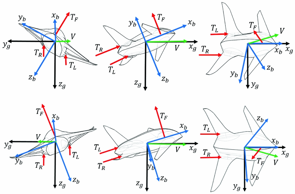
With direct-force control technology, the Microraptor has three flight states, which are hovering, cruising and transition flight. Under the hovering condition, the lift fan is activated and the vectoring nozzles are deflected to 90°. Propulsive forces and controls are predominant and flow angles range from −180° to 180°. Under forward-flight condition, power is provided by thrust vector engines and vectoring nozzles are tilted to 0°, producing thrust along the longitudinal axis. Since the lift fan is inactive, control is primarily achieved by aero surface deflections and weight is mainly countered by aerodynamic forces. Under transition flight condition, thrust vector nozzles work at intermediate tilt angles. The UAV's attitude and flight path are controlled by the coordinate of aerodynamic effectors and thrust vector engine effectors. Illustrations of three flight states are shown in Fig. 2.
Figure 2. Illustration of three flight states.
To reduce flight-test cost and facilitate the control-system research, a 2:1 shrink ratio prototype is manufactured (Fig. 3). The aircraft is entirely electrically powered, with lithium-polymer batteries for 8 minutes cruising and 4 minutes hovering. The scale model has the same control mechanism as the conceptual model. In the scale model, each wing has an aileron and a total of four aerodynamic surfaces. The lift fan is located at the front of the fuselage. A control vane connected to the shaft is equipped under the lift fan, which can swing left and right from −12° to 12°. The thrust vector engine nozzles can swing up for 15° and swing down for 90°. Combined with the lift fan and the thrust vector engines, there are a total of six control inputs the for power system, which are TF, TL, TR, δF, δL and δR. All control effectors can be changed independently, providing redundancy for control strategies.
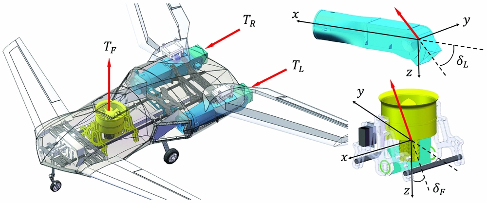
Figure 3. Microraptor 2:1 scale model.
Necessary flight tests have been conducted on the prototype (Fig. 4). To ensure the authenticity and rationality of the control model, the configuration data, aerodynamic data and engine thrust data used in this paper are all based on the estimation and measurement of the scale model. The Microraptor's overall characteristics are presented in Table 1.
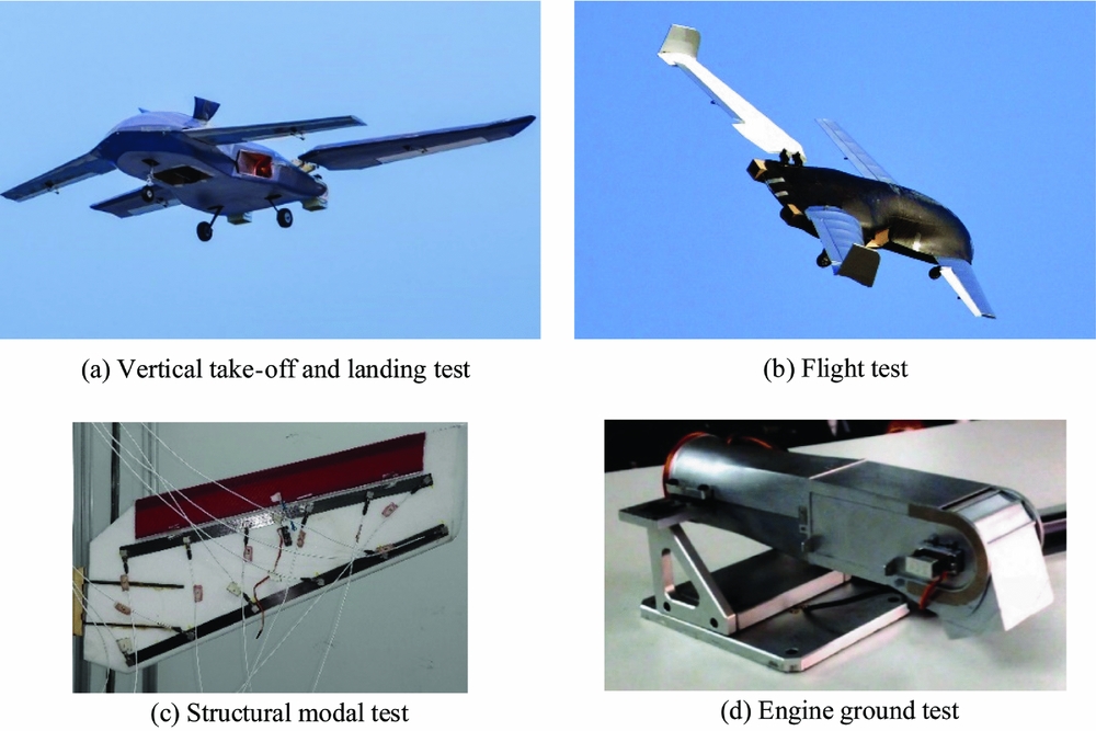
Figure 4. Tests of the Microraptor prototype.
Table 1 Prototype basic data
In the case of no wind-tunnel experiment, aerodynamic data of the UAV were obtained by aerodynamic estimation, CFD calculation and flight data identification together. The mapping relationship between effectors (control surfaces/actuators), aerodynamic forces and moments are usually non-linear. In this paper, to meet the requirement of the control allocation algorithm, polynomial approximation is used to fit the aerodynamic data curve between effector deflections and moment coefficients. This will alleviate the need for the use of large look-up tables, and hence ensure higher accuracy as well as speed up the control allocation computational process.
3.0 VEHICLE CONTROL MODEL
A dynamic-inversion-based method is developed to control the UAV. The model is established in right-handed (RH) Cartesian coordinate systems. The flight vehicle and flat earth reference frame are assumed to be rigid and inertial, respectively. The body reference frame (Oxbybzb), flat earth reference frame (Oxgygzg), and velocity reference frame (Oxvyvzv) are shown in Fig. 5.
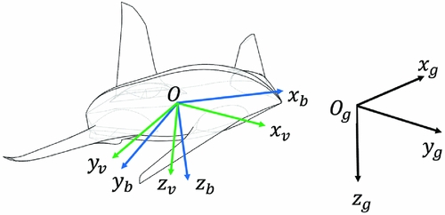
Figure 5. UAV reference frames.
First, the 6 DOF problem is transferred into a two-time-scale problem based on singular perturbation theory. According to the physical characteristics and dynamic relationship between the control inputs, from outer to inner, the control loops are the translational kinematics control loop, the translational dynamics control loop, the rotational kinematics control loop and the rotational dynamics control loop, respectively. The dynamic inversion method is used for loop control separately. The first stage of the two-stage progressive optimal control allocation method is adopted in the translational dynamics control loop (Equations (1) and (2)) to make the engine-vectored-thrust in body axes (Tx, Ty, Tz) and wind angles (α, β, μ) approach the desired value. For simplification, the effect of aerodynamic control surfaces deflection on linear acceleration is neglected in the control design, of which the effect is considered a disturbance on aerodynamic coefficients.
 $$\begin{equation}
\left[ \arraycolsep5pt\begin{array}{@{}c@{}}
{{{\dot{V}}_{{\rm{des}}}}}\\
{{{\dot{\chi }}_{{\rm{des}}}}}\\
{{{\dot{\gamma }}_{{\rm{des}}}}} \end{array} \right] =
\left[ \arraycolsep5pt\begin{array}{@{}c@{}}
{{{\dot{V}}_c}}\\
{{{\dot{\chi }}_c}}\\
{{{\dot{\gamma }}_c}} \end{array}\right] +
\left[ \arraycolsep5pt\begin{array}{@{}ccc@{}}
{{K_V}}&{}&{}\\
{}&{{K_\chi }}&{}\\
{}&{}&{{K_\gamma }}\\
\end{array} \right]\left[
\arraycolsep5pt\begin{array}{@{}c@{}} {{V_{\rm{c}}} - V}\\
{{\chi _c} - \chi }\\
{{\gamma _c} - \gamma } \end{array} \right],
\end{equation}$$
$$\begin{equation}
\left[ \arraycolsep5pt\begin{array}{@{}c@{}}
{{{\dot{V}}_{{\rm{des}}}}}\\
{{{\dot{\chi }}_{{\rm{des}}}}}\\
{{{\dot{\gamma }}_{{\rm{des}}}}} \end{array} \right] =
\left[ \arraycolsep5pt\begin{array}{@{}c@{}}
{{{\dot{V}}_c}}\\
{{{\dot{\chi }}_c}}\\
{{{\dot{\gamma }}_c}} \end{array}\right] +
\left[ \arraycolsep5pt\begin{array}{@{}ccc@{}}
{{K_V}}&{}&{}\\
{}&{{K_\chi }}&{}\\
{}&{}&{{K_\gamma }}\\
\end{array} \right]\left[
\arraycolsep5pt\begin{array}{@{}c@{}} {{V_{\rm{c}}} - V}\\
{{\chi _c} - \chi }\\
{{\gamma _c} - \gamma } \end{array} \right],
\end{equation}$$
 $$\begin{equation}
\left[ \arraycolsep5pt\begin{array}{@{}c@{}}
{{{\dot{V}}_{{\rm{des}}}}}\\
{V{{\dot{\chi }}_{{\rm{des}}}}\cos \gamma }\\
{ - V{{\dot{\gamma }}_{{\rm{des}}}}}\\
\end{array} \right] =
\frac{1}{m}\left(
{\bf L}_{\bf kb}\left( {\bm \alpha }_{\bm c},{\bm \beta }_{\bm c},{\bm \mu }_{\bm c} \right)
\left[
\arraycolsep5pt\begin{array}{@{}c@{}}
{{T_x}}\\
{{T_y}}\\
{{T_z}}\\
\end{array} \right] + {\bf L}_{\bf ka}\left( {\bm \alpha }_{\bm c},{\bm \beta }_{\bm c},{\bm \mu }_{\bm c} \right)
\left[ \arraycolsep5pt\begin{array}{@{}c@{}}
{ - D\left( {{\alpha _c}} \right)}\\
{C\left( {{\beta _c}} \right)}\\
{ - L\left( {{\alpha _c}} \right)} \\
\end{array} \right] +
m{\bf L}_{\bf kg}\left[
\arraycolsep5pt\begin{array}{@{}c@{}}
0\\
0\\
g \\
\end{array} \right] \right)
\end{equation}$$
$$\begin{equation}
\left[ \arraycolsep5pt\begin{array}{@{}c@{}}
{{{\dot{V}}_{{\rm{des}}}}}\\
{V{{\dot{\chi }}_{{\rm{des}}}}\cos \gamma }\\
{ - V{{\dot{\gamma }}_{{\rm{des}}}}}\\
\end{array} \right] =
\frac{1}{m}\left(
{\bf L}_{\bf kb}\left( {\bm \alpha }_{\bm c},{\bm \beta }_{\bm c},{\bm \mu }_{\bm c} \right)
\left[
\arraycolsep5pt\begin{array}{@{}c@{}}
{{T_x}}\\
{{T_y}}\\
{{T_z}}\\
\end{array} \right] + {\bf L}_{\bf ka}\left( {\bm \alpha }_{\bm c},{\bm \beta }_{\bm c},{\bm \mu }_{\bm c} \right)
\left[ \arraycolsep5pt\begin{array}{@{}c@{}}
{ - D\left( {{\alpha _c}} \right)}\\
{C\left( {{\beta _c}} \right)}\\
{ - L\left( {{\alpha _c}} \right)} \\
\end{array} \right] +
m{\bf L}_{\bf kg}\left[
\arraycolsep5pt\begin{array}{@{}c@{}}
0\\
0\\
g \\
\end{array} \right] \right)
\end{equation}$$
In the rotational dynamics control loop (Equations (3) and (4)), the sum of aerodynamic surface moments ls, ms, ns and thrust vector moments lT, mT, nT are calculated. As the Microraptor contains lots of effectors of power-system and aerodynamic surfaces, the rotational dynamic control loop first generates virtual commands lc, mc, nc, and the allocation of control effectors are made in a separate module.
 $$\begin{equation}
\left[ {\arraycolsep5pt\begin{array}{@{}*{1}{c}@{}} {{{\dot{p}}_{{\rm{des}}}}}\\ {{{\dot{q}}_{{\rm{des}}}}}\\ {{{\dot{r}}_{{\rm{des}}}}} \end{array}} \right] = \left[ {\arraycolsep5pt\begin{array}{@{}*{3}{c}@{}} {{K_p}}&{}&{}\\ {}&{{K_q}}&{}\\ {}&{}&{{K_r}} \end{array}} \right]\left[ {\arraycolsep5pt\begin{array}{@{}*{1}{c}@{}} {{p_c} - p}\\ {{q_c} - q}\\ {{r_c} - r} \end{array}} \right],\vspace*{-15pt}
\end{equation}$$
$$\begin{equation}
\left[ {\arraycolsep5pt\begin{array}{@{}*{1}{c}@{}} {{{\dot{p}}_{{\rm{des}}}}}\\ {{{\dot{q}}_{{\rm{des}}}}}\\ {{{\dot{r}}_{{\rm{des}}}}} \end{array}} \right] = \left[ {\arraycolsep5pt\begin{array}{@{}*{3}{c}@{}} {{K_p}}&{}&{}\\ {}&{{K_q}}&{}\\ {}&{}&{{K_r}} \end{array}} \right]\left[ {\arraycolsep5pt\begin{array}{@{}*{1}{c}@{}} {{p_c} - p}\\ {{q_c} - q}\\ {{r_c} - r} \end{array}} \right],\vspace*{-15pt}
\end{equation}$$
 $$\begin{equation}
{\bf I} \cdot \left[ {\arraycolsep5pt\begin{array}{@{}*{1}{c}@{}} {{{\dot{p}}_{{\rm{des}}}}}\\ {{{\dot{q}}_{{\rm{des}}}}}\\ {{{\dot{r}}_{{\rm{des}}}}} \end{array}} \right] + \left[ {\arraycolsep5pt\begin{array}{@{}*{1}{c}@{}} p\\ q\\ r \end{array}} \right] \times \left( {{\bf I} \cdot \left[ {\arraycolsep5pt\begin{array}{@{}*{1}{c}@{}} p\\ q\\ r \end{array}} \right]} \right) - \left[ {\arraycolsep5pt\begin{array}{@{}*{1}{c}@{}} {{l_A}}\\ {{m_A}}\\ {{n_A}} \end{array}} \right] = \left[ {\arraycolsep5pt\begin{array}{@{}*{1}{c}@{}} {{l_s}}\\ {{m_s}}\\ {{n_s}} \end{array}} \right] + \left[ {\arraycolsep5pt\begin{array}{@{}*{1}{c}@{}} {{l_T}}\\ {{m_T}}\\ {{n_T}} \end{array}} \right] = \left[ {\arraycolsep5pt\begin{array}{@{}*{1}{c}@{}} {{l_c}}\\ {{m_c}}\\ {{n_c}} \end{array}} \right]
\end{equation}$$
$$\begin{equation}
{\bf I} \cdot \left[ {\arraycolsep5pt\begin{array}{@{}*{1}{c}@{}} {{{\dot{p}}_{{\rm{des}}}}}\\ {{{\dot{q}}_{{\rm{des}}}}}\\ {{{\dot{r}}_{{\rm{des}}}}} \end{array}} \right] + \left[ {\arraycolsep5pt\begin{array}{@{}*{1}{c}@{}} p\\ q\\ r \end{array}} \right] \times \left( {{\bf I} \cdot \left[ {\arraycolsep5pt\begin{array}{@{}*{1}{c}@{}} p\\ q\\ r \end{array}} \right]} \right) - \left[ {\arraycolsep5pt\begin{array}{@{}*{1}{c}@{}} {{l_A}}\\ {{m_A}}\\ {{n_A}} \end{array}} \right] = \left[ {\arraycolsep5pt\begin{array}{@{}*{1}{c}@{}} {{l_s}}\\ {{m_s}}\\ {{n_s}} \end{array}} \right] + \left[ {\arraycolsep5pt\begin{array}{@{}*{1}{c}@{}} {{l_T}}\\ {{m_T}}\\ {{n_T}} \end{array}} \right] = \left[ {\arraycolsep5pt\begin{array}{@{}*{1}{c}@{}} {{l_c}}\\ {{m_c}}\\ {{n_c}} \end{array}} \right]
\end{equation}$$
With virtual commands transmitted to the optimal control allocation module, the second stage of the two-stage progressive optimal control allocation method is applied. In this module, the engines’ thrust, vectoring nozzles and aileron deflection angles are calculated, and the desired control force and moments are generated. A conceptual block diagram of the dynamic inversion controller is shown in Fig. 6.

Figure 6. Conceptual block diagram of the control system.
4.0 DIRECT-FORCE OPTIMAL CONTROL ALLOCATION
4.1 Optimisation problem description
Control allocation is useful for control of over-actuated systems. In this paper, the sequential quadratic programming (SQP) algorithm is adopted in two-stage progressive optimal control allocation method. The SQP algorithm has been one of the most successful general algorithms for solving non-linear constrained optimisation problems, owing to its convergence(Reference Boggs and Tolle15). The important feature of SQP is that a primal problem in the design variable space is transformed to a quadratic programming (QP) formulation, a Taylor series is used for the objective and constraint functions, and then a quadratic approximate objective function with linearised constraints is used to create a direction finding of the form shown below(Reference Ghenaiet16).
 $$\begin{equation}
J = {\rm{min}}\frac{1}{2}{{\bf d}^T}{\bf H}\left( {{x_k}} \right){\bf d} + \nabla {f}{\left( {{x_k}} \right)^T}{\bf d,}\vspace*{-15pt}
\end{equation}$$
$$\begin{equation}
J = {\rm{min}}\frac{1}{2}{{\bf d}^T}{\bf H}\left( {{x_k}} \right){\bf d} + \nabla {f}{\left( {{x_k}} \right)^T}{\bf d,}\vspace*{-15pt}
\end{equation}$$
 $$\begin{equation}
s.t.\left\{ {\arraycolsep5pt\begin{array}{@{}*{1}{c}@{}} {{\bm{g}_i}\left( {{x_k}} \right) + \nabla {\bm{g}_i}{{\left( {{x_k}} \right)}^T} = 0\ \left( {i = 1,2, \ldots ,l} \right)}\\[8pt] {{\bm{g}_i}\left( {{x_k}} \right) + \nabla {\bm{g}_i}{{\left( {{x_k}} \right)}^T} \ge 0\ \left( {i = l + 1,L + 2, \ldots ,m} \right)} \end{array}} \right.
\end{equation}$$
$$\begin{equation}
s.t.\left\{ {\arraycolsep5pt\begin{array}{@{}*{1}{c}@{}} {{\bm{g}_i}\left( {{x_k}} \right) + \nabla {\bm{g}_i}{{\left( {{x_k}} \right)}^T} = 0\ \left( {i = 1,2, \ldots ,l} \right)}\\[8pt] {{\bm{g}_i}\left( {{x_k}} \right) + \nabla {\bm{g}_i}{{\left( {{x_k}} \right)}^T} \ge 0\ \left( {i = l + 1,L + 2, \ldots ,m} \right)} \end{array}} \right.
\end{equation}$$
In Equations (5) and (6), H(xk) is a positive definite approximation of the Hessian, d is the search direction in the k th iteration, and f, g are an objective function and constraints, respectively. The problem is solved iteratively. A line search is used to find a new point for every iteration, such that a merit function will have a lower value at the new point. If optimality is not achieved, H(xk) is updated according to the modified Broyden–Fletcher–Goldfarb–Shanno (BFGS) formula(Reference Powell17). More details about this technique are available in Refs Reference Boggs and Tolle15 and Reference Powell17.
Generally, control allocation problem can be stated as a constrained least square problem. To bring the requirements corresponding to the flight task into the optimisation objectives, the objective function in the first stage of the two-stage progressive optimal control allocation method is designed as
 $$\begin{equation}
J = {\left[ {\arraycolsep5pt\begin{array}{@{}*{1}{c}@{}} {{w_{\alpha 1}}}\\ {{w_{\beta 1}}}\\ {{w_{\mu 1}}} \end{array}} \right]^T}\left[ {\arraycolsep5pt\begin{array}{@{}*{1}{c}@{}} {{{\left( {\alpha - {\alpha _0}} \right)}^2}}\\ {{{\left( {\beta - {\beta _0}} \right)}^2}}\\ {{{\left( {\mu - {\mu _0}} \right)}^2}} \end{array}} \right] + {\left[ {\arraycolsep5pt\begin{array}{@{}*{1}{c}@{}} {{w_{\alpha 2}}}\\ {{w_{\beta 2}}}\\ {{w_{\mu 2}}} \end{array}} \right]^T}\left[ {\arraycolsep5pt\begin{array}{@{}*{1}{c}@{}} {{{\left( {\alpha - {\alpha _{{\rm{balance}}}}} \right)}^2}}\\ {{\beta ^2}}\\ {{\mu ^2}} \end{array}} \right] + {\left[ {\arraycolsep5pt\begin{array}{@{}*{1}{c}@{}} {{w_{Tx}}}\\ {{w_{Ty}}}\\ {{w_{Tz}}} \end{array}} \right]^T}\left[ {\arraycolsep5pt\begin{array}{@{}*{1}{c}@{}} {T_x^2}\\ {T_y^2}\\ {T_z^2} \end{array}} \right],
\end{equation}$$
$$\begin{equation}
J = {\left[ {\arraycolsep5pt\begin{array}{@{}*{1}{c}@{}} {{w_{\alpha 1}}}\\ {{w_{\beta 1}}}\\ {{w_{\mu 1}}} \end{array}} \right]^T}\left[ {\arraycolsep5pt\begin{array}{@{}*{1}{c}@{}} {{{\left( {\alpha - {\alpha _0}} \right)}^2}}\\ {{{\left( {\beta - {\beta _0}} \right)}^2}}\\ {{{\left( {\mu - {\mu _0}} \right)}^2}} \end{array}} \right] + {\left[ {\arraycolsep5pt\begin{array}{@{}*{1}{c}@{}} {{w_{\alpha 2}}}\\ {{w_{\beta 2}}}\\ {{w_{\mu 2}}} \end{array}} \right]^T}\left[ {\arraycolsep5pt\begin{array}{@{}*{1}{c}@{}} {{{\left( {\alpha - {\alpha _{{\rm{balance}}}}} \right)}^2}}\\ {{\beta ^2}}\\ {{\mu ^2}} \end{array}} \right] + {\left[ {\arraycolsep5pt\begin{array}{@{}*{1}{c}@{}} {{w_{Tx}}}\\ {{w_{Ty}}}\\ {{w_{Tz}}} \end{array}} \right]^T}\left[ {\arraycolsep5pt\begin{array}{@{}*{1}{c}@{}} {T_x^2}\\ {T_y^2}\\ {T_z^2} \end{array}} \right],
\end{equation}$$
where the first term takes the last sampling period state α0, β0, μ0 to avoid the jump of wind angles; the second term tends to minimise the wind angles during flight; likewise, the third term tends to minimise the power system thrust during flight. In optimal iteration, if the constrains are not satisfied, it may lead to an infeasible solution. To alleviate such possibility, the constraint is relaxed. J is minimised subject to the constraints in Equation (2), and the limitations of effectors are not considered. If the control allocation results exceed the effector's range, the weight of the exceed effector will change. The outputs of the translational dynamics control loop are virtual commands, the attainability of control demands due to the position or rate saturation of the actuators will be considered in the second stage of the two-stage progressive optimal control allocation method.
4.2 Weight selection scheme
In different missions, such as vertical take-off, transition flight and cruising, effectors’ responsibility and using prize are different, and therefore it is necessary to develop a task-tailored control allocation strategy to achieve the optimum dynamic response for each task. The optimal control allocation can realise multiple objectives with different effectors’ weight, such as minimum wind angle change during the transition flight and minimum thrust consumption during the take-off phase. According to the characteristics of the different mission, a self-correction analytic hierarchy process (SC-AHP) is proposed to obtain the weights of the objective function.
The analytic hierarchy process (AHP) is a structured technique for organising and analysing complex decisions. It provides a comprehensive and rational framework for representing and quantifying its elements, relating those elements to overall goals, and evaluating alternative solutions. First, we decompose the decision problem into a hierarchy of more easily comprehensive sub-problems, each of which can be analysed independently. The effectors in objective function (Equation (7)) are divided into three different homogeneous groups S 1, S 2, S 3, where their weights are  $[{\!\!\!\arraycolsep5pt\begin{array}{*{20}{c}} {{w_{\alpha 1}}}&{{w_{\beta 1}}}&{{w_{\mu 1}}}\end{array}}\!\!\!]$,
  $[\!\!\! {\arraycolsep5pt\begin{array}{*{20}{c}} {{w_{\alpha 2}}}&{{w_{\beta 2}}}&{{w_{\mu 2}}}\end{array}}\!\!\!]$ and
  $[\!\!\!{\arraycolsep5pt\begin{array}{*{20}{c}} {{w_{Tx}}}&{{w_{Ty}}}&{{w_{Tz}}}\end{array}}\!\!\!]$. Let A 1, A 2, A 3, depict the set of priorities of groups S 1, S 2, S 3. The quantified judgements on pairs of Ai, Aj, are represented by a 3-by-3 matrix A = [aij], ij = 1, 2, 3, where aij indicates the priority of Si relative to Sj. If Si is judged to be of equal relative priority to Sj then aij = 1; If Si is judged to be less prior than Sj then aij > 1, else 0 < aij < 1. In order to maintain consistency in the judgements, the aij should be defined by the rule in Equation (8):
 $$\begin{equation}
{a_{ij}} = \frac{{{a_{ik}}}}{{{a_{jk}}}}\ \;\left( {i,j,k = 1,2,3} \right)
\end{equation}$$
$$\begin{equation}
{a_{ij}} = \frac{{{a_{ik}}}}{{{a_{jk}}}}\ \;\left( {i,j,k = 1,2,3} \right)
\end{equation}$$
In making comparisons, aij comes from the human's judgements about the elements' relative meaning and importance. In the Microraptor's control system the judgements matrixes for typical flight tasks are artificially designed offline and stored in an expert system. For example, the value of aij in Equation (9) reflects the smooth change of the wind angle, and the priority of aerodynamic control is higher than direct-force control. With the flight-state inputs, the expert system will create the relative judgements matrix based on artificially designed judgement matrixes.
 $$\begin{equation}
{\bf A} = \left[ {{a_{ij}}} \right] = \left[ {\arraycolsep5pt\begin{array}{@{}*{3}{c}@{}} {{a_{11}}}&{{a_{12}}}&{{a_{13}}}\\ {{a_{21}}}&{{a_{22}}}&{{a_{23}}}\\ {{a_{31}}}&{{a_{32}}}&{{a_{33}}} \end{array}} \right] = \left[ {\arraycolsep5pt\begin{array}{@{}*{3}{c}@{}} 1&5&{2.5}\\ {0.2}&1&{0.5}\\ {0.4}&2&1 \end{array}} \right]
\end{equation}$$
$$\begin{equation}
{\bf A} = \left[ {{a_{ij}}} \right] = \left[ {\arraycolsep5pt\begin{array}{@{}*{3}{c}@{}} {{a_{11}}}&{{a_{12}}}&{{a_{13}}}\\ {{a_{21}}}&{{a_{22}}}&{{a_{23}}}\\ {{a_{31}}}&{{a_{32}}}&{{a_{33}}} \end{array}} \right] = \left[ {\arraycolsep5pt\begin{array}{@{}*{3}{c}@{}} 1&5&{2.5}\\ {0.2}&1&{0.5}\\ {0.4}&2&1 \end{array}} \right]
\end{equation}$$
Use the judgement matrix to determine the priority of the groups S 1, S 2, S 3, which can be calculated by Equation (10). It is worth noting that the process of determining the weights is carried out under the premise that the optimisation variable in different groups are on same unit magnitude. The optimisation variables in S 1 represent the change of wind angle. The optimisation variables in S 2 are the size of the wind angle. The optimisation variables in S 3 are the direct force in body axis. Therefore, to ensure the validity of the objective function, the correction factors should be introduced to make the weights in the same order of magnitude (Equation (11)).
 $$\begin{equation}
{a_i} = \sqrt[3]{{{a_{i1}}{a_{i2}}{a_{i3}}}},\vspace*{-15pt}
\end{equation}$$
$$\begin{equation}
{a_i} = \sqrt[3]{{{a_{i1}}{a_{i2}}{a_{i3}}}},\vspace*{-15pt}
\end{equation}$$
 $$\begin{equation}
\left[ {\arraycolsep5pt\begin{array}{@{}*{1}{c}@{}} {{A_1}}\\ {{A_2}}\\ {{A_3}} \end{array}} \right] = \frac{1}{{\mathop \sum \nolimits_{i = 1}^3 {a_i}}}\left[ {\arraycolsep5pt\begin{array}{@{}*{1}{c}@{}} {{a_1} \cdot {{10}^2}}\\ {{a_2}}\\ {{a_3} \cdot {{10}^{ - 4}}} \end{array}} \right]
\end{equation}$$
$$\begin{equation}
\left[ {\arraycolsep5pt\begin{array}{@{}*{1}{c}@{}} {{A_1}}\\ {{A_2}}\\ {{A_3}} \end{array}} \right] = \frac{1}{{\mathop \sum \nolimits_{i = 1}^3 {a_i}}}\left[ {\arraycolsep5pt\begin{array}{@{}*{1}{c}@{}} {{a_1} \cdot {{10}^2}}\\ {{a_2}}\\ {{a_3} \cdot {{10}^{ - 4}}} \end{array}} \right]
\end{equation}$$
After judging the priority of different groups, the subordinate priority of effectors in each group is determined. Take the group S 1 as an example, bij indicates the priority of effector Ni relative to effector Nj in group S 1. Like the previous method, the subordinate priority of effectors in S 1 can be determined by the judgement matrix. Since the effectors in same group are on the same order of magnitude, the correction factors are not needed.
 $$\begin{equation}
{B_i} = \frac{{{b_i}}}{{\mathop \sum \nolimits_{i = 1}^3 {b_i}}} = \frac{{\sqrt[3]{{{b_{i1}}{b_{i2}}{b_{i3}}}}}}{{\mathop \sum \nolimits_{i = 1}^3 {b_i}}}
\end{equation}$$
$$\begin{equation}
{B_i} = \frac{{{b_i}}}{{\mathop \sum \nolimits_{i = 1}^3 {b_i}}} = \frac{{\sqrt[3]{{{b_{i1}}{b_{i2}}{b_{i3}}}}}}{{\mathop \sum \nolimits_{i = 1}^3 {b_i}}}
\end{equation}$$
Similarly, the priority of effectors in S 2 are represented by Ci (i = 1, 2, 3), and the priority of effectors in S 3 are represented by Di (i = 1, 2, 3). In the final step of the process, the weight of optimisation variables in the objective function can be calculated by Equation (13).
 $$\begin{equation}
\arraycolsep5pt\begin{array}{@{}*{5}{c}@{}} {\left[\!\!{\arraycolsep5pt\begin{array}{*{20}{c}} {{w_{\alpha 1}}}&{{w_{\beta 1}}}&{{w_{\mu 1}}} \end{array}}\!\! \right] = {A_1}\left[\!\!{\arraycolsep5pt\begin{array}{*{20}{c}} {{B_1}}&{{B_2}}&{{B_3}} \end{array}}\!\! \right]}\\\\[-10pt] {\left[\!\!{\arraycolsep5pt\begin{array}{*{20}{c}} {{w_{\alpha 2}}}&{{w_{\beta 2}}}&{{w_{\mu 2}}} \end{array}}\!\! \right] = {A_2}\left[\!\! {\arraycolsep5pt\begin{array}{*{20}{c}} {{C_1}}&{{C_2}}&{{C_3}} \end{array}}\!\! \right]}\\\\[-10pt] {\left[\!\!{\arraycolsep5pt\begin{array}{*{20}{c}} {{w_{Tx}}}&{{w_{Ty}}}&{{w_{Tz}}} \end{array}}\!\! \right] = {A_3}\left[\!\! {\arraycolsep5pt\begin{array}{*{20}{c}} {{D_1}}&{{D_2}}&{{D_3}} \end{array}}\!\! \right]} \end{array}
\end{equation}$$
$$\begin{equation}
\arraycolsep5pt\begin{array}{@{}*{5}{c}@{}} {\left[\!\!{\arraycolsep5pt\begin{array}{*{20}{c}} {{w_{\alpha 1}}}&{{w_{\beta 1}}}&{{w_{\mu 1}}} \end{array}}\!\! \right] = {A_1}\left[\!\!{\arraycolsep5pt\begin{array}{*{20}{c}} {{B_1}}&{{B_2}}&{{B_3}} \end{array}}\!\! \right]}\\\\[-10pt] {\left[\!\!{\arraycolsep5pt\begin{array}{*{20}{c}} {{w_{\alpha 2}}}&{{w_{\beta 2}}}&{{w_{\mu 2}}} \end{array}}\!\! \right] = {A_2}\left[\!\! {\arraycolsep5pt\begin{array}{*{20}{c}} {{C_1}}&{{C_2}}&{{C_3}} \end{array}}\!\! \right]}\\\\[-10pt] {\left[\!\!{\arraycolsep5pt\begin{array}{*{20}{c}} {{w_{Tx}}}&{{w_{Ty}}}&{{w_{Tz}}} \end{array}}\!\! \right] = {A_3}\left[\!\! {\arraycolsep5pt\begin{array}{*{20}{c}} {{D_1}}&{{D_2}}&{{D_3}} \end{array}}\!\! \right]} \end{array}
\end{equation}$$
In the solving process of optimisation function, if the optimisation variable is found to exceed the setting range, the weight of the exceed variable relative to other optimisation variables in the same group will be improved, and the importance of the group to which the exceed variable belongs relative to other groups is also improved. The judgement matrix is changed to generate a new weight for the next calculation.
5.0 EFFECTORS OPTIMAL-CONTROL ALLOCATION
5.1 Optimisation problems description
In the rotational dynamics control loop, the sum of  ${[ {\arraycolsep3pt\begin{array}{*{20}{c}} {{l_s}}&{{m_s}}&{{n_s}} \end{array}}\! ]^T}$and
  ${[ {\arraycolsep3pt\begin{array}{*{20}{c}} {{l_T}}&{{m_T}}&{{n_T}} \end{array}} ]^T}$can be calculated. Since the forces and moments generated by the engine system are coupled, it is necessary to consider the
  ${[{\arraycolsep3pt\begin{array}{*{20}{c}} {{T_x}}&{{T_y}}&{{T_z}}\end{array}}]^T}$in the control allocator that maps the total control command on individual actuators. The dynamic model of thrust vector engine system can be expressed as
 $$\begin{equation}
\left\{ {\arraycolsep5pt\begin{array}{@{}*{1}{c}@{}} {{T_x} = {T_L}\cos {\delta _L} + {T_R}\cos {\delta _R}}\\[7pt] {{T_y} = {T_F}\sin {\delta _F}}\\[7pt] {{T_z} = {T_L}\sin {\delta _L} + {T_R}\sin {\delta _R} - {T_F}\cos {\delta _F}}\\[7pt] {{l_T} = - {T_L}\sin {\delta _L}{d_{yt}} + {T_R}\sin {\delta _R}{d_{yt}}}\\[7pt] {{m_T} = \left( {{T_L}\sin {\delta _L} + {T_L}\sin {\delta _L}} \right){d_{xt}} + {T_F}\cos {\delta _F}{d_{xf}}}\\[7pt] {{n_T} = \left( {{T_L}\cos {\delta _L} - {T_R}\cos {\delta _R}} \right){d_{yt}} + {T_F}\sin {\delta _F}{d_{xf}}} \end{array}} \right.,
\end{equation}$$
$$\begin{equation}
\left\{ {\arraycolsep5pt\begin{array}{@{}*{1}{c}@{}} {{T_x} = {T_L}\cos {\delta _L} + {T_R}\cos {\delta _R}}\\[7pt] {{T_y} = {T_F}\sin {\delta _F}}\\[7pt] {{T_z} = {T_L}\sin {\delta _L} + {T_R}\sin {\delta _R} - {T_F}\cos {\delta _F}}\\[7pt] {{l_T} = - {T_L}\sin {\delta _L}{d_{yt}} + {T_R}\sin {\delta _R}{d_{yt}}}\\[7pt] {{m_T} = \left( {{T_L}\sin {\delta _L} + {T_L}\sin {\delta _L}} \right){d_{xt}} + {T_F}\cos {\delta _F}{d_{xf}}}\\[7pt] {{n_T} = \left( {{T_L}\cos {\delta _L} - {T_R}\cos {\delta _R}} \right){d_{yt}} + {T_F}\sin {\delta _F}{d_{xf}}} \end{array}} \right.,
\end{equation}$$
where TL, TR, TF δR, δL, δF are actual control effectors needed for displacement, which are determined from the desired moments and forces. In case the lift fan is off, the model can be expressed as
 $$\begin{equation}
\left\{ {\arraycolsep5pt\begin{array}{@{}*{1}{c}@{}} {{T_x} = {T_L}\cos {\delta _L} + {T_R}\cos {\delta _R}}\\[7pt] {{T_z} = {T_L}\sin {\delta _L} + {T_R}\sin {\delta _R}}\\[7pt] {{l_T} = - {T_L}\sin {\delta _L}{d_{yt}} + {T_R}\sin {\delta _R}{d_{yt}}}\\[7pt] {{m_T} = \left( {{T_L}\sin {\delta _L} + {T_R}\sin {\delta _R}} \right){d_{xt}}}\\[7pt] {{n_T} = \left( {{T_L}\cos {\delta _L} - {T_R}\cos {\delta _R}} \right){d_{yt}}} \end{array}} \right.
\end{equation}$$
$$\begin{equation}
\left\{ {\arraycolsep5pt\begin{array}{@{}*{1}{c}@{}} {{T_x} = {T_L}\cos {\delta _L} + {T_R}\cos {\delta _R}}\\[7pt] {{T_z} = {T_L}\sin {\delta _L} + {T_R}\sin {\delta _R}}\\[7pt] {{l_T} = - {T_L}\sin {\delta _L}{d_{yt}} + {T_R}\sin {\delta _R}{d_{yt}}}\\[7pt] {{m_T} = \left( {{T_L}\sin {\delta _L} + {T_R}\sin {\delta _R}} \right){d_{xt}}}\\[7pt] {{n_T} = \left( {{T_L}\cos {\delta _L} - {T_R}\cos {\delta _R}} \right){d_{yt}}} \end{array}} \right.
\end{equation}$$
To fulfil the control demand in the translational dynamics control loop, it's necessary to satisfy the target value of Tx, Ty, Tz at priority. To ensure the value of the control effectors can be solved, the constraint of control allocation is relaxed by introducing the tolerance range of  ${[\! {\arraycolsep3pt\begin{array}{*{20}{c}} {{l_T}}&{{m_T}}&{{n_T}}\end{array}}\!]^T}$. As the total amount of control moments are determined in Equation (16), and the range of aerodynamic moments can be calculated from the control surface deflection angles, therefore the available range of thrust vector moments can be calculated from the aerodynamic moments range (Equation (17)).
 $$\begin{equation}
\left[ {\arraycolsep5pt\begin{array}{@{}*{1}{c}@{}} {{l_s}}\\ {{m_s}}\\ {{n_s}} \end{array}} \right] + \left[ {\arraycolsep5pt\begin{array}{@{}*{1}{c}@{}} {{l_T}}\\ {{m_T}}\\ {{n_T}} \end{array}} \right] = \left[ {\arraycolsep5pt\begin{array}{@{}*{1}{c}@{}} {{l_c}}\\ {{m_c}}\\ {{n_c}} \end{array}} \right],
\end{equation}$$
$$\begin{equation}
\left[ {\arraycolsep5pt\begin{array}{@{}*{1}{c}@{}} {{l_s}}\\ {{m_s}}\\ {{n_s}} \end{array}} \right] + \left[ {\arraycolsep5pt\begin{array}{@{}*{1}{c}@{}} {{l_T}}\\ {{m_T}}\\ {{n_T}} \end{array}} \right] = \left[ {\arraycolsep5pt\begin{array}{@{}*{1}{c}@{}} {{l_c}}\\ {{m_c}}\\ {{n_c}} \end{array}} \right],
\end{equation}$$
 $$\begin{equation}
\left[{\arraycolsep5pt\begin{array}{@{}*{1}{c}@{}} {{l_c}}\\ {{m_c}}\\ {{n_c}} \end{array}} \right] - {\left[{\arraycolsep5pt\begin{array}{@{}*{1}{c}@{}} {{l_s}}\\ {{m_s}}\\ {{n_s}} \end{array}} \right]_{{\rm{max}}}} \le \left[ {\arraycolsep5pt\begin{array}{@{}*{1}{c}@{}} {{l_T}}\\ {{m_T}}\\ {{n_T}} \end{array}} \right] \le \left[ {\arraycolsep5pt\begin{array}{@{}*{1}{c}@{}} {{l_c}}\\ {{m_c}}\\ {{n_c}} \end{array}} \right] - {\left[ {\arraycolsep5pt\begin{array}{@{}*{1}{c}@{}} {{l_s}}\\ {{m_s}}\\ {{n_s}} \end{array}} \right]_{{\rm{min}}}}
\end{equation}$$
$$\begin{equation}
\left[{\arraycolsep5pt\begin{array}{@{}*{1}{c}@{}} {{l_c}}\\ {{m_c}}\\ {{n_c}} \end{array}} \right] - {\left[{\arraycolsep5pt\begin{array}{@{}*{1}{c}@{}} {{l_s}}\\ {{m_s}}\\ {{n_s}} \end{array}} \right]_{{\rm{max}}}} \le \left[ {\arraycolsep5pt\begin{array}{@{}*{1}{c}@{}} {{l_T}}\\ {{m_T}}\\ {{n_T}} \end{array}} \right] \le \left[ {\arraycolsep5pt\begin{array}{@{}*{1}{c}@{}} {{l_c}}\\ {{m_c}}\\ {{n_c}} \end{array}} \right] - {\left[ {\arraycolsep5pt\begin{array}{@{}*{1}{c}@{}} {{l_s}}\\ {{m_s}}\\ {{n_s}} \end{array}} \right]_{{\rm{min}}}}
\end{equation}$$
In Equation (17),  $[\!{\arraycolsep3pt\begin{array}{*{20}{c}} {{l_s}}&{{m_s}}&{{n_s}}\end{array}}\!]_{{\rm{max}}}^T$ and
  $[\!{\arraycolsep3pt\begin{array}{*{20}{c}} {{l_s}}&{{m_s}}&{{n_s}}\end{array}}\!]_{{\rm{min}}}^T$ are the maximum and minimum aerodynamic control moments, respectively. The Microraptor doesn't contain rudder, so ns = 0, nT = nc. The control allocation method is changed into the solving of non-linear optimisation problem with four equality constrains (Tx, Ty, Tz, nT) and two inequality constrains (lT, mT). The objective function of the second-stage optimal control allocation method is designed as
 $$\begin{equation}
J = {\left[ {\arraycolsep5pt\begin{array}{@{}*{1}{c}@{}} {{w_{TL}}}\\ {{w_{TR}}}\\ {{w_{TF}}} \end{array}} \right]^T}\left[ {\arraycolsep5pt\begin{array}{@{}*{1}{c}@{}} {T_L^2}\\ {T_R^2}\\ {T_F^2} \end{array}} \right] + {\left[ {\arraycolsep5pt\begin{array}{@{}*{1}{c}@{}} {{w_{\delta L}}}\\ {{w_{\delta R}}}\\ {{w_{\delta F}}} \end{array}} \right]^T}\left[ {\arraycolsep5pt\begin{array}{@{}*{1}{c}@{}} {\delta _L^2}\\ {\delta _R^2}\\ {\delta _F^2} \end{array}} \right],
\end{equation}$$
$$\begin{equation}
J = {\left[ {\arraycolsep5pt\begin{array}{@{}*{1}{c}@{}} {{w_{TL}}}\\ {{w_{TR}}}\\ {{w_{TF}}} \end{array}} \right]^T}\left[ {\arraycolsep5pt\begin{array}{@{}*{1}{c}@{}} {T_L^2}\\ {T_R^2}\\ {T_F^2} \end{array}} \right] + {\left[ {\arraycolsep5pt\begin{array}{@{}*{1}{c}@{}} {{w_{\delta L}}}\\ {{w_{\delta R}}}\\ {{w_{\delta F}}} \end{array}} \right]^T}\left[ {\arraycolsep5pt\begin{array}{@{}*{1}{c}@{}} {\delta _L^2}\\ {\delta _R^2}\\ {\delta _F^2} \end{array}} \right],
\end{equation}$$
where the weights are determined by the self-correction analytic hierarchy process (SC-AHP), which was described earlier. The weights can be adjusted according to the different flight condition and task, ensuring the control allocator can generate reasonable results.
5.2 Effectors limitation
The constraints of the effector's rate and position limits are not considered in the optimal allocation of the above two control loops. In the SQP algorithm, the more the constraints, the slower the solution, and incomplete constraints may cause the controller to produce an unreasonable solution to satisfy local constraints. Therefore, the two-stage progressive optimal control allocation method is designed to solve the optimisation problem with no constrains of TL, TR, TF, δL, δR, δF. After the solving optimisation problem, transferring the value of δL, δR, δF into [ − 0.5π, 0.5π], and adjusting the effector's value, the control inputs are guaranteed not to violate the rate or position limits. If the control inputs reach saturation, and the allocation algorithms could not achieve the desired dynamics, the weight in objective function will be adjusted in the next calculation to adapt to the capabilities of the control effectors.
 $$\begin{equation}
\left\{ {\arraycolsep5pt\begin{array}{@{}*{1}{c}@{}} {{\rm{if}}\;{T_i} \ge {T_{i{\rm{max}}}},\;{T_i} = {T_{i{\rm{max}}}}}\\[7pt] {{\rm{if}}\;{T_i} \le {T_{i{\rm{min}}}},\;{T_i} = {T_{i{\rm{min}}}}}\\[7pt] {{\rm{if}}\;{\delta _i}\left( {{t_n}} \right) \ge \min \left( {{\delta _i}\left( {{t_{n - 1}}} \right) + {{\dot{\delta }}_{i{\rm{max}}}}\Delta t,\;{\delta _i}{\rm{max}}} \right),\;{\delta _i} = {\rm{min}}\left( {{\delta _i}\left( {{t_{n - 1}}} \right) + {{\dot{\delta }}_{i{\rm{max}}}}\Delta t,\;{\delta _i}{\rm{max}}} \right)}\\[7pt] {{\rm{if}}\;{\delta _i}\left( {{t_n}} \right) \le \max \left( {{\delta _i}\left( {{t_{n - 1}}} \right) - {{\dot{\delta }}_{i{\rm{max}}}}\Delta t,\;{\delta _i}{\rm{min}}} \right),\;{\delta _i} = {\rm{max}}\left( {{\delta _i}\left( {{t_{n - 1}}} \right) - {{\dot{\delta }}_{i{\rm{max}}}}\Delta t,\;{\delta _i}{\rm{min}}} \right)} \end{array}} \right.
\end{equation}$$
$$\begin{equation}
\left\{ {\arraycolsep5pt\begin{array}{@{}*{1}{c}@{}} {{\rm{if}}\;{T_i} \ge {T_{i{\rm{max}}}},\;{T_i} = {T_{i{\rm{max}}}}}\\[7pt] {{\rm{if}}\;{T_i} \le {T_{i{\rm{min}}}},\;{T_i} = {T_{i{\rm{min}}}}}\\[7pt] {{\rm{if}}\;{\delta _i}\left( {{t_n}} \right) \ge \min \left( {{\delta _i}\left( {{t_{n - 1}}} \right) + {{\dot{\delta }}_{i{\rm{max}}}}\Delta t,\;{\delta _i}{\rm{max}}} \right),\;{\delta _i} = {\rm{min}}\left( {{\delta _i}\left( {{t_{n - 1}}} \right) + {{\dot{\delta }}_{i{\rm{max}}}}\Delta t,\;{\delta _i}{\rm{max}}} \right)}\\[7pt] {{\rm{if}}\;{\delta _i}\left( {{t_n}} \right) \le \max \left( {{\delta _i}\left( {{t_{n - 1}}} \right) - {{\dot{\delta }}_{i{\rm{max}}}}\Delta t,\;{\delta _i}{\rm{min}}} \right),\;{\delta _i} = {\rm{max}}\left( {{\delta _i}\left( {{t_{n - 1}}} \right) - {{\dot{\delta }}_{i{\rm{max}}}}\Delta t,\;{\delta _i}{\rm{min}}} \right)} \end{array}} \right.
\end{equation}$$
In Equation (19), δi(t n − 1) represents the effector's position in last state,  ${\dot{\delta }_{i{\rm{max}}}}$ represents the maximum deflection speed of the effector. The
  $[\!{\arraycolsep3pt\begin{array}{*{20}{c}} {{l_T}}&{{m_T}}&{{n_T}}\end{array}}\!]_{{\rm{real}}}^T$ can be calculated by limited optimal results, and then the corresponding aerodynamic surface moments can be calculated by Equation (20). Finally, the deflection angles of aerodynamic control surface
  ${[\!\! {\arraycolsep5pt\begin{array}{*{20}{c}} {{\delta _a}}&{{\delta _e}}&0 \end{array}}\!\! ]^T}$ can be calculated.
 $$\begin{equation}
\left[ {\arraycolsep5pt\begin{array}{@{}*{1}{c}@{}} {{l_s}}\\ {{m_s}}\\ {{n_s}} \end{array}} \right]_{{\rm{real}}}^T = {\left[ {\arraycolsep5pt\begin{array}{@{}*{1}{c}@{}} {{l_c}}\\ {{m_c}}\\ {{n_c}} \end{array}} \right]^T} - \left[ {\arraycolsep5pt\begin{array}{@{}*{1}{c}@{}} {{l_T}}\\ {{m_T}}\\ {{n_T}} \end{array}} \right]_{{\rm{real}}}^T
\end{equation}$$
$$\begin{equation}
\left[ {\arraycolsep5pt\begin{array}{@{}*{1}{c}@{}} {{l_s}}\\ {{m_s}}\\ {{n_s}} \end{array}} \right]_{{\rm{real}}}^T = {\left[ {\arraycolsep5pt\begin{array}{@{}*{1}{c}@{}} {{l_c}}\\ {{m_c}}\\ {{n_c}} \end{array}} \right]^T} - \left[ {\arraycolsep5pt\begin{array}{@{}*{1}{c}@{}} {{l_T}}\\ {{m_T}}\\ {{n_T}} \end{array}} \right]_{{\rm{real}}}^T
\end{equation}$$
A conceptual block diagram of the second-stage progressive optimal control allocation method is shown in Fig. 7.

Figure 7. Conceptual block diagram of optimal control allocation.
6.0 SIMULATION
The flight simulation consists of two examples. In each example, a high manoeuverability flight path is designed. The simulation is conducted to make the Microraptor follow the path, aiming to assess the effectiveness of the control system and verify the Microraptor's manoeuverability in transition flight.
6.1 Example of vertical take-off & transition flight
The flight path is designed in Equation (21). In the Z axis, the reference path climbs at 2 m/s from the start and lasts for 40 seconds. Then the climb rate turns to 0 m/s, and the aircraft makes altitude hold flight. In the Y axis, the reference path is unchanged. In the X axis, the velocity is changed in sinusoidal lasting for 280 seconds, and the maximum velocity is 31 m/s and minimum velocity is 1 m/s. The aircraft takes three times of transition from hovering to cruising to follow the reference path.
 $$\begin{equation}
\arraycolsep5pt\begin{array}{@{}*{1}{c}@{}} {{V_{cx}} = 15\sin \left( {t/30 - 0.5\pi } \right) + 16}\\[7pt] {{V_{cy}} = 0}\\[7pt] {{V_{cz}} = \left\{ {\arraycolsep5pt\begin{array}{@{}*{2}{c}@{}} {\arraycolsep5pt\begin{array}{*{20}{c}} { - 2}&{0 \le t \le 40} \end{array}}\\[7pt] {\arraycolsep5pt\begin{array}{*{20}{c}} 0&{\ \ \ \ \ t > 40} \end{array}} \end{array}} \right.} \end{array}
\end{equation}$$
$$\begin{equation}
\arraycolsep5pt\begin{array}{@{}*{1}{c}@{}} {{V_{cx}} = 15\sin \left( {t/30 - 0.5\pi } \right) + 16}\\[7pt] {{V_{cy}} = 0}\\[7pt] {{V_{cz}} = \left\{ {\arraycolsep5pt\begin{array}{@{}*{2}{c}@{}} {\arraycolsep5pt\begin{array}{*{20}{c}} { - 2}&{0 \le t \le 40} \end{array}}\\[7pt] {\arraycolsep5pt\begin{array}{*{20}{c}} 0&{\ \ \ \ \ t > 40} \end{array}} \end{array}} \right.} \end{array}
\end{equation}$$
Considering the uncertainty of aerodynamic coefficients and the presence of turbulence, the disturbance force is added to the model to assess the robustness of the controller. The force is represented in Equation (22), where μ is a random number between 0 and 1, and the sample time is 3 seconds.
 $$\begin{equation}
\arraycolsep5pt\begin{array}{@{}*{1}{c}@{}} {{F_{xd}} = 5\mu \sin \left( {0.2\pi t} \right)}\\[7pt] {{F_{yd}} = 5\mu \sin \left( {0.2\pi t} \right)}\\[7pt] {{F_{zd}} = 3\mu \sin \left( {0.2\pi t} \right)} \end{array}
\end{equation}$$
$$\begin{equation}
\arraycolsep5pt\begin{array}{@{}*{1}{c}@{}} {{F_{xd}} = 5\mu \sin \left( {0.2\pi t} \right)}\\[7pt] {{F_{yd}} = 5\mu \sin \left( {0.2\pi t} \right)}\\[7pt] {{F_{zd}} = 3\mu \sin \left( {0.2\pi t} \right)} \end{array}
\end{equation}$$
In this example, two weight strategies have been proposed. The first is designed to make the attitude stable and the Euler angle smaller during flight. The second is designed to use less lift-fan and thrust vectoring nozzle deflection during flight. The comparison and analysis of the two strategies have been made. The reference path is designed to test the aircraft's capability of task-oriented manoeuverability and robustness in transition flight.
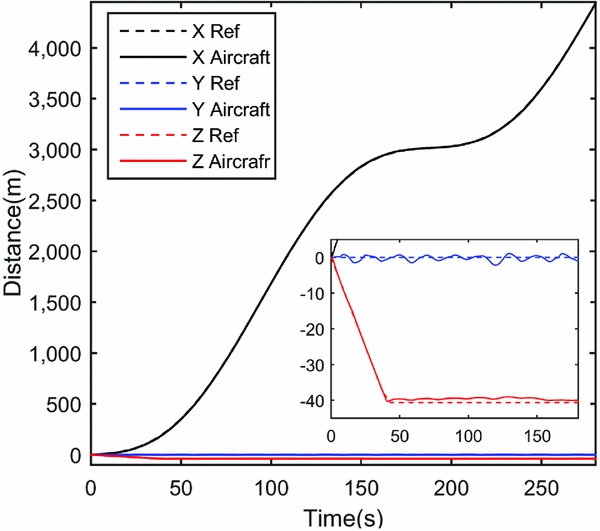
The simulation result shows that both weight strategies can follow the reference flight path well. The flight path and velocity information of the first strategy are shown in Figs 8–10, and the second strategy are similar. In Figs 11 and 12, the dotted lines represent the simulation results without force disturbance, and the solid lines, which fluctuate around the dotted lines, represent the simulation results considering the force disturbance. Under the action of the control system, the error caused by the disturbance is reduced and the overall trend of the reference flight path can be well tracked.

Figure 8. Flight path.

Figure 9. Three-axis velocity.

Figure 10. Flight path angles.

Figure 11. Wind angles.

Figure 12. Engine system states.
The wind angle and power system state of two strategies during flight are shown in Figs 11 and 12. In climbing phase, the first strategy is selected to keep the pitch angle small and stable, the angle-of-attack (α) is minus and nearly changed with flight path angle (γ). With the increasing of forward speed, α is increased first and then decreased to make aircraft hold flight altitude. The second strategy is used to increase the α rapidly at the start to reduce the use of lift fan and vectoring nozzle deflection.
From 120 seconds to 250 seconds, the UAV reduces the velocity and transfers into low-speed cruising state. For the first strategy, UAV in deceleration process increases the angle-of-attack to maintain a sufficient lift and balance the weight of aircraft. With further deceleration, based on the optimisation results, the lift fan begins to work and the vectoring nozzles sweep down. Angle-of-attack is reduced to keep the UAV attitude in normal flight state. In the acceleration process, the thrust of the lift fan decreases to zero and the vectoring nozzles turn to horizontal smoothly, and the angle-of-attack is changed to corporate the flight state. For the second strategy, the angle-of-attack increases from 0 to 87 degrees to produce sufficient lift and the engine's thrust is used to balance the weight of the aircraft.
From 60 seconds to 130 seconds, when the UAV's velocity is higher than the minimum cruising speed, the lift fan could be manually turned off. In strategy one, the lift fan is not manually turned off, which results in the lift fan's control vane vibrating, as shown in Fig. 12(c), even though the lift fan's thrust as calculated by the optimal allocation algorithm is small. In strategy two, the lift fan is manually turned off, it can be seen clearly in Fig. 12(d) that the TF and δF are equal to zero, which avoids the vibration of control van and makes the Microraptor cruise like a conventional aircraft.
Figure 13 and Table 2 and Table 3 illustrate the vehicle's flight states from 117 seconds to 260.2 seconds. As shown in Fig. 13, the difference of the manoeuver process caused by different weight selection strategy is obvious. It proves the effectiveness of two-stage progressive optimal control allocation method and weight selection scheme.

Figure 13. Illustration of vehicle's attitude in low-speed cruising.
Table 2 Flight states for the first strategy

Table 3 Flight states for the second strategy

6.2 Example of lateral Manoeuver in transition flight
Example 2 is mainly used to simulate the flight path tracking in the city's low-altitude flight environment and to test the UAV's lateral manoeuverability in the low-speed cruising phase. In the X axis direction of the ground coordinate system, the reference flight path is accelerated at the initial speed of 5 m/s, which reflects the transition process of the UAV from hovering to normal cruising. In Y axis direction, the velocity of reference flight path is made a wide range of fluctuations, which reflects the manoeuver process of UAV to avoid the urban buildings. In Z axis direction, the reference flight path is maintained at the height of 40 m. The results of simulation are shown in Fig. 14.

Figure 14. Simulation results for lateral manoeuver in transition flight.
In Fig. 14(d) the UAV's roll, pitch, yaw angles are changed simultaneously during the manoeuver process, which indicates the control system uses the change of attitude to generate aerodynamic force to facilitate manoeuvering. Figures 14(e) and (f) show the change of engine thrust and nozzles/vane deflection angles, respectively. The thrust-vector power system provides both control moments and direct-control forces for UAV manoeuvering. Therefore, the thrust vectoring and aerodynamic force control the UAV synergistically in the path tracking process.
Take the flight time at 16.03 seconds and 25.71 seconds as the samples to analyse, where the lateral manoeuvering is fierce, the change rate of the velocity in Y-axis direction is high, and the largest side slip angle occurred. Table 4 and Fig. 15 show the UAV's flight status of two moments, respectively. We can find that the UAV adjusts the nose-pointing direction consistent with the reference path by changing the roll angle and angle-of-attack. Meanwhile, aerodynamic forces and direct forces provided by power system help UAV make the same movement trend with reference path. The above analysis can be verified by Fig. 14(d). In Fig. 14(d), the change pattern of yaw angle (ψ) is similar with kinematic azimuth angle (χ), but ψ is slightly delayed, which is caused by the direct force control. Observing the side slip angle (β) of the two moments, we find that the deflection direction of the side slip angle is in opposite trend of UAV's lateral movement. The reason is that, in low-speed cruising, the thrust must compensate for the lift to maintain the flight altitude, the side slip angle is solved to help power system generate proper thrust component in ground Z axis direction. All of the control inputs and UAV's attitude are determined by the control system's optimal results.
Table 4 Flight states


Figure 15. Illustration of flight attitude and thrust vectoring (three views).
The simulation result shows satisfactory performance of the designed UAV in lateral high-manoeuvering path tracking. The control system can optimise the UAV's attitude in different flight time and make full use of aerodynamic force. It also allocates the redundant effector's efficiency and generates control moments and force accurately. Compared with conventional aircraft, the UAV discussed in this paper can follow the flight path with lower velocity and higher manoeuverability. The controller can exploit the dynamic characters of the power system in the maximum way.
7.0 CONCLUSION
This work is focused on the flight vehicle's high manoeuverability control strategy in transition flight. A two-stage progressive optimal control allocation method is developed to solve the problem of engine-vectored thrust and aerodynamic force assignments in direct-force control, as well as the control management of the effector redundancy. Simulation results show that with the direct-force control technique, UAV possesses superior manoeuverability in transition flight and is suitable for applications in complex flight environment. According to different task requirements, the weight selection scheme can generate corresponding values for objective function, which obviously changes the flight state. The numerical optimisation process can converge rapidly, and the computation time for each control cycle is rational and suitable for onboard use. Overall, with the designed control system, UAV can exploit the characteristics of VTOL engine system, allocate each effector reasonably, and exhibit satisfactory control performance with high efficiency. In the future, the control method presented in this paper will be transplanted on the Microraptor's flight controller. A flight test needs to be further conducted to validate the effectiveness of the proposed control algorithm.
ACKNOWLEDGEMENTS
This work is supported by the Aeronautical Science Foundation of China Grant 2016ZA72001. The authors would like to thank all the members of the Microraptor Works, Key Lab of Dynamics and Control of Flight Vehicle, Ministry of Education, School of Aerospace Engineering, Beijing Institute of Technology.