


NOMENCLATURE
- LAA
Large Amphibious Aircraft
- UAV
Unmanned Aerial Vehicle
- SA
Total area of the search area
- Sf
Area searched by the aircraft
- Sd
Area size of the repeated search
- Sm
Missing search area
- ax, ay, az
aircraft’s guidance command
- δx, δy, δz
Control rudder deflection angles
1.0 INTRODUCTION
Maritime search and rescue are capabilities for locating a shipwreck or a lost aircraft. Presently, air search and rescue is effective only within the offshore area; search and rescue missions for outer ocean areas require helicopters.
Helicopter searches and rescues are mainly used in long-sea missions. Because helicopters have no sea rescue capability and must wait for ships to arrive, the rescue time is lengthy and the survival probability of personnel is low. Large amphibious aircraft(Reference Li, Cai and Xie1) is a single-hull four-engine turboprop developed by China. Its flight time and range performance far exceed helicopters, and the platform has a strong carrying capacity. It has the capability to integrate maritime search and rescue, which can achieve rapid speed in the ocean search and rescue missions.
To maximise the use of flight characteristics of large amphibious aircraft and achieve fast and effective long-sea search and rescue missions, effective maritime search route planning algorithms become essential for amphibious aircraft search and rescue. The current search route planning methods can be divided into the following two categories according to actual task conditions: coverage search route planning without prior information and waypoint search route planning with prior information.
Search route planning problems include t the required searchable areas without prior conditions, so that the radar along the path can cover all search areas with the largest area. Currently, the coverage search route planning problem is widely used in the field of ground and underwater robots and unmanned aerial vehicles. Although the applications are varied, the principle of these methods is same. Enric Galceran(Reference Enric and Marc2) summarised several existing methods for covering search route planning, such as trapezoidal decomposition(Reference Oksanen and Visala3), staggered decomposition, Morse decomposition(Reference Ercan, Howie, Alfred, Prasad and Douglas4) and other methods, dividing the searched area into different complete blocks, and for the method of meshing, summarised the wave front(Reference Shivashankar, Jain, Kuter and Nau5), spanning tree(Reference Lee, Baek, Choi and Oh6) and neural network method(Reference Luo and Yang7), and gave the advantages and disadvantages of each method. Paulo(Reference Tobias, Shuaiby, Naoki and Oliver8) used a genetic algorithm to solve the obstacle avoidance path planning problem of the robot in a limited space. Yan Zheping(Reference Zheping, Jingwen and Juan9) improved the traditional particle swarm algorithm and combined predictive control with particle swarm to realise multi-AUV patrol route planning. Ai Bing(Reference Bing and Rui10) gave the auxiliary planning algorithm of the helicopter maritime search and rescue route, and proposed the traditional trapezoidal, square and sector search route.
The problem of waypoint search-route planning is to plan the search route under the existing prior conditions. The route requires passing all required waypoints and meeting all constraints. This type of problem is mainly applied to drones, missiles and other aircraft. Li Pei(Reference Li and Duan11) adopted the gravitational search algorithm to realise the optimal route planning of UAVs in complex environments. Chen Mou(Reference Mou, Jian and Changsheng12) studied a UAV three-dimensional route-planning method based on an improved ant colony algorithm for a UAV penetration problem. Ma Xiangling(Reference Ma, Chen and Lei13) improved the A* algorithm combined with the data link and introduced the inertial weight coefficient to realise the UAV evading terrain route planning. Liang Xiao(Reference Liang, Wang, Meng and Chen14) used a uniform grid method to model the real 3D environment and used the ant colony algorithm to complete the route-planning problem. Liang Xiao(Reference Liang, Wang, Li and Lv15) used the principle of flowing water to avoid rocks to realise the problem of UAV three-dimensional route planning. Wei Ruixuan(Reference Wei, Xu, Wang and Lv16) used the Laguerre graph algorithm for route pre-planning and, on this basis, simplified the scope of the secondary planning space as well as used the improved La-star algorithm to implement the secondary route planning in the simplified planning space.
The sea search path planning problem of large amphibious aircraft is essentially a multi-constrained coverage route planning problem. From the current domestic and foreign route planning algorithms, the waypoint search route planning algorithm has certain reference significance, but it does not consider the coverage area. If it is directly applied to the coverage route planning problem, it will result in the increase of computation time for the performance index. The coverage route planning method does not involve the re-search rate index, which is an important search index; for the missing search rate index, it does not consider that the turning process may cause part of the area to be missed. And the current research is mainly aimed at the field of robotics. For large amphibious aircraft, the flight constraints need to be considered during the planning process. It can be seen that the planning of long-sea search and rescue routes for large amphibious aircraft is still in the preliminary research stage. According to the actual performance parameters of the large amphibious aircraft, this paper introduces the traceback path index to improve the dynamic planning based optimal route planning algorithm applied for maritime search route planning under the constraints of the no-fly zone, in which the minimum value of the comprehensive performance index for the re-search rate, the miss-search rate and the flight range can be obtained. Compared with the traditional search schemes, the optimal route planning performance index in this paper is the smallest, and the search efficiency is the highest.
2.0 PROBLEM DESCRIPTION
The problem of optimal search route planning for large amphibious aircraft at sea requires the aircraft to complete all search tasks with the shortest flight range, minimizing the area of missing and repeated search, which is essential for a coverage route planning problem. The problem of optimal search route planning for large amphibious aircraft above the sea is described in detail as follows: large amphibious aircraft take off from the starting airport (p x, p y); complete a full coverage search in a specified area of the sea; and return to the original airport (p x, p y). The aircraft maintains level flight during the search. The level flight search altitude is h s, the level flight search speed is v s, and the radar search radius is r s. The aircraft needs to avoid all no-fly zones during the search flight process to maximise the coverage of the searched area and minimise the missed search rate.
The performance indicators of large-scale amphibious aircraft sea search route planning are divided into three items: the shortest total flight range, the largest total search area, and the smallest re-search area. The comprehensive performance index function is shown in formula (1):
 \begin{align} J = \mathop {\min }\limits_{(x(t),y(t))} \left({k_1} \cdot {l_f} + {k_2} \cdot \frac{{{S_A} - {S_f}}}{{{S_A}}} + {k_3} \cdot \frac{{{S_d}}}{{{S_A}}}\right) \end{align}
where l f is the total flight range, including the flight distance of the aircraft from the airport to the search area and back to the airport; S A is the total area of the search area; S f is the area searched by the aircraft; S d is the area size of the repeated search, and k 1, k 2, and k 3 are the weight ratios. According to actual search requirements and expert experience, the settings are as shown in formula (2):
 \begin{align} k_{1}=\frac{2r_{s}}{S_{A}}, \quad k_{2}=5, \quad k_{3}=1\end{align}
At the same time, the search route planning of large amphibious aircraft needs to meet the following constraints:
(a) The minimum turning radius r min of large amphibious aircraft, or the maximum usable overload n max;
(b) Large amphibious aircraft are not allowed to enter the no-fly zone (air defense zone, storm zone, etc.) during the search.
Large amphibious aircraft sea optimal search route planning problem requires planning its flight path (x(t), y(t)) to make the performance index formula (1) the smallest and meet all constraints. The maritime optimal search route planning problem for large amphibious aircraft is a multi-constraint coupled nonlinear optimisation problem, in which two or more repeated search areas are defined. As radar is continuously scanning in the search process, it is difficult to formulate the area of re-search. To better solve the problem of maritime search route planning, this paper transforms the problem to a certain extent.
2.1 The model of the search sea area
In view of the particularity of various possible sea search and rescue missions, the wreck search area is large, the planned search area is usually a rectangle, and the rectangle parameter is the rectangle vertex (s xi, s yi), i = 1, 2, 3, 4, The sides of the rectangle are a and b. According to the search radar radius of the large amphibious aircraft and the actual mission requirements, the original search sea area is divided into a grid network, and the side length of each grid is twice the radar search radius, that is, 2r s. When the aircraft flies from the centre of a certain grid point to the centre of its connected grid point, the radar will scan all the areas between the two grids, and this part will neither miss nor re-search, as shown in Fig. 1, so the grid network can transform the original search route planning problem into a discrete planning problem, and the planned path should pass through all network grid points without repetition. The network grid point is the centre point of each grid, which is the red point in Fig. 1.

Figure 1. Search zone while aircraft fly pass grids.
The attribute parameters of each grid point in the grid network are shown in Table 1.
Table 1 The attribute parameters of grid

Among them, grid connected domains generally have three situations according to their locations: corner points, edge points, and interior points. The corner points, edge points, and interior points are, respectively, located at the four corners, four sides and interior of the search area. The connected domains are shown in Fig. 2, and the arrow indicates the connected domain direction of the current grid.

Figure 2. Mesh connected domain.
2.2 No-fly zone model
In the search sea area, there may be various no-fly zones, such as severe weather conditions, island armed areas, etc. The no-fly zone will affect the connected domain of the grid. As shown in Figs. 3 and 4, in the case of two no-fly zones, square and circular, the second and fourth grids in Fig. 3 are no longer connected, Fig. 4 is no longer connected between the first grid and the third grid. In addition, the existence of a no-fly zone will also affect the index of the re-search rate. Therefore, the performance index of flying between grid points with a no-fly zone is different from the situation without a no-fly zone. The calculation of the performance index can be referred to section 2.3 later in this article.
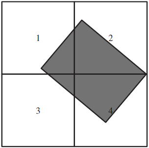
Figure 3. Square no-flying zone.

Figure 4. Circular no-fly zone.
The no-fly zone considered in this paper is mainly divided into two types: square and circular. Suppose the centre point of the square no-fly zone is (x c, y c), and the side lengths are a, b (a ≥ b), and the rotation angle of the square no-fly zone is  $\theta(-\pi/2\leq\theta\pi/2)$. When the coordinates (x, y) satisfy formula (3), the point is considered to be outside the square no-fly zone.
 \begin{align}
\left[
\begin{array}{c}
X\\[2pt]
Y\end{array}
\right] & = T\left( \theta \right)\left[
\begin{array}{c}{x - {x_c}}\\[2pt]
{y - {y_c}}\end{array}
\right]\nonumber\\[6pt]
T\left( \theta \right) & = \left[
\begin{array}{c@{\quad}c}
\cos \theta & - \sin \theta\\[4pt]
\sin \theta & \cos \theta
\end{array}
\right]\\[4pt]
& \left| {X_p} \right| \gt \frac{a}{2}, \left| {{Y_p}} \right| \gt \frac{b}{2}\nonumber
\end{align}
\begin{align}
\left[
\begin{array}{c}
X\\[2pt]
Y\end{array}
\right] & = T\left( \theta \right)\left[
\begin{array}{c}{x - {x_c}}\\[2pt]
{y - {y_c}}\end{array}
\right]\nonumber\\[6pt]
T\left( \theta \right) & = \left[
\begin{array}{c@{\quad}c}
\cos \theta & - \sin \theta\\[4pt]
\sin \theta & \cos \theta
\end{array}
\right]\\[4pt]
& \left| {X_p} \right| \gt \frac{a}{2}, \left| {{Y_p}} \right| \gt \frac{b}{2}\nonumber
\end{align}
Assuming that the centre point of the circular no-fly zone is (x s, y s) and the radius is r, when the coordinates (x p, y p) satisfy formula (4), the point is considered to be outside the circular no-fly zone.
 \begin{align}\sqrt {{{(x - {x_s})}^2} + {{(y - {y_s})}^2}} \gt r\\[-10pt] \nonumber\end{align}
2.3 Calculation of missing search rate and re-search rate
The missing search rate and the re-search rate are important indicators for the large amphibious aircraft sea route search. To ensure the efficiency of the sea search route, it is necessary to minimise the missing search rate and the re-search rate. Under the grid network model, the calculation methods of missing search rate and re-search rate are divided into the following two cases.
2.3.1 There is no no-fly zone
When there is no no-fly zone between the grid points, the large amphibious aircraft flying between grid points can be divided into straight flight and turning flight. As shown in Figs. 5 and 6, during the turning flight of the aircraft, there will be an area that cannot be searched. Considering the importance of the missing search rate and the re-search rate, the turning point of the turning flight trajectory needs to be optimised.

Figure 5. Search zone of aircraft with straight flight line.

Figure 6. Search zone of aircraft with turning flight.
Generally speaking, we believe that under the grid network model the waypoint of the aircraft is equivalent to the centre point of the grid. This article considers the reduction of the missing search in certain areas during the turn, and the search waypoints for the aircraft in the grid are optimised. For maritime search and rescue, the ratio of missing search rate and re-search rate is generally 1:5. By optimising the distance l from the centre of the grid in Fig. 7, the following turning costs are minimised:
 \begin{equation} J = \mathop {\min }\limits_{x,y} \left(5 \cdot {S_m} + {S_d}\right) \end{equation}
Among them, S m is the missing search area and S d is the re-search area.

Figure 7. Missing search zone and re-search zone of aircraft with turning flight in no no-flying zone.
When l = 0.2634r s, the performance index of Equation (5) is the smallest.
2.3.2 There is a no-fly zone
When the aircraft passes through the grid point containing the no-fly zone, it needs to fly around the no-fly zone. Take the third grid in Fig. 4 as an example, when the aircraft enters the grid from the west, since the north grid is completely occupied by the threat zone, the current grid’s connected domains only have east and south directions. As shown in Fig. 8, the red dotted line is flying south, and the green dashed line is flying east. The trajectory of the aircraft needs to fly to the next search grid while avoiding the no-fly zone.

Figure 8. Re-search zone of aircraft in no-flying zone.
The performance index function for flying between grids with no-fly zones is designed as follows.
When the flight direction is east-west or north-south, similar to the green dashed line in the Fig. 8, the re-search area is the shaded area of the grid line in the figure, and the area of this zone is related to the longest distance d 1 of its trajectory from the central axis. The calculation method is shown in Equation (6); when the flight direction needs to be turned, similar to the red dashed line in the figure, its re-search area is the diagonally shaded area. The area of this zone is related to the longest distance d 2 of its trajectory on the diagonal. The calculation method of the re-search area for this situation is shown in Equation (7):
 \begin{equation}\hspace*{-90pt}{S_{re\_stg}} = \sqrt {2{r_s}{d_1} - d_1^2} \cdot ({r_s} - {d_1})\hspace*{80pt}\end{equation}
 \begin{align}
{S_{re\_turn}} & = \left\{
\begin{array}{l@{\quad}c}
0, & {d_2} \le \left(\sqrt 2 - 1\right){r_s}\\[8pt]
\left(\frac{\pi }{4} - \theta \right)r_s^2 - \left(\cos \theta \cdot {r_s} - \frac{{dh}}{{\sqrt 2 }}\right) \cdot \frac{{dh}}{{\sqrt 2 }}, & {d_2} \left(\sqrt{2} - 1\right){r_s}
\end{array} \right.\\[5pt]
dh & = {r_s} - {d_2}\qquad \theta = {\rm{arc}}\sin \left( {\frac{{dh}}{{\sqrt 2 {r_s}}}} \right)\nonumber
\end{align}
\begin{align}
{S_{re\_turn}} & = \left\{
\begin{array}{l@{\quad}c}
0, & {d_2} \le \left(\sqrt 2 - 1\right){r_s}\\[8pt]
\left(\frac{\pi }{4} - \theta \right)r_s^2 - \left(\cos \theta \cdot {r_s} - \frac{{dh}}{{\sqrt 2 }}\right) \cdot \frac{{dh}}{{\sqrt 2 }}, & {d_2} \left(\sqrt{2} - 1\right){r_s}
\end{array} \right.\\[5pt]
dh & = {r_s} - {d_2}\qquad \theta = {\rm{arc}}\sin \left( {\frac{{dh}}{{\sqrt 2 {r_s}}}} \right)\nonumber
\end{align}
where S re_stg is the re-search area in the straight flight direction; S re_turn is the re-search area in the turning flight direction; d 1 is the farthest distance from the central axis of the flight trajectory to avoid the no-fly zone in the straight flight direction; d 2 is the distance from the centre point on the diagonal of the flight trajectory avoiding the no-fly zone in the turning flight direction; and d h and  $\theta$ are intermediate variables and have no actual physical meaning.
3.0 SEARCH ROUTE PLANNING ALGORITHM
In view of the particularity of this problem, through the construction and transformation of the network model in the previous section, this paper transforms the large amphibious aircraft search path planning problem into a discrete multi-stage optimisation problem. The effect of re-search rate and miss-search rate can be solved by the order and direction of the passed grids. Aiming at the discrete multi-stage optimisation problem, this paper introduces a reverse dynamic programming algorithm to solve it, and improves and optimises it. The traceback index is introduced in the performance index to solve the problem of grid point selection under the same index condition. The specific search route planning algorithm is discussed in the following sections.
3.1 Search route planning algorithm based on improved dynamic programming
In the improved dynamic programming algorithm in this paper, the network model is divided into three layers, namely network (Net), step (Step), and grid (Point), and the parameter definitions are shown in Table 2.
Table 2 Parameter table of route planning algorithm

Based on the grid network construction in Table 2, the calculation steps of the search route planning algorithm used in this project are as follows:
Step 1. Read in map information, search for environmental information data such as threat areas.
Step 2. Construct a search grid network, establish a grid model and connected domains according to the aircraft search characteristics and threat zone information.
Step 3. Read in the initial and terminal airport positions (x 0, y 0).
Step 4. Select the search grid closest to the initial airport as the starting grid, record its grid coordinates as
 $(i_{x\mathit{0}}, i_{y\mathit{0}})$ speed as $(i_{vx}, i_{vy})$, and current number of steps Step = 1.
Step 5. Calculate the connected domain
$\Omega\{(i_{xN}, i_{yN})\}$ of all positions $\Omega\{(i_{xC}, i_{yC})\}$ of the current step.Step 6. Calculate the performance indicators of all connected domain grids
$(i_{xN}, i_{yN})$ of Step+1, $(i_{xN}, i_{yN})$ is the connected domain grid of grids $(i_{xC}, i_{yC})$, and the performance indicators will vary according to different situations:
(a) When there is no no-fly zone in the grid (i xN, i yN), the performance index of the grid (i xN, i yN) is calculated as follows.
(8)
\begin{align}
J({x_N},{y_N}) & = J({x_C},{y_C}) + \left\{ \begin{array}{c@{\quad}l} 1, & \left| {\Delta iv} \right| = 0\\[3pt]
- 0.4146, & \left| {\Delta iv} \right| = \sqrt 2 \\[3pt]
- 4, & \left| {\Delta iv} \right| = 2 \end{array} \right.\\[4pt]
{\overrightarrow {iv}_{\!N}} & = (i{x_N},i{y_N}) - (i{x_C},i{y_C})\nonumber\\[4pt]
\Delta \overrightarrow {iv} & = {\overrightarrow {iv}_{\!N}} - {\overrightarrow {iv}_{\!C}}\nonumber\end{align}
where (i xC, i yC) is the currently calculated grid point; J(xC, yC) is the performance index of the point (i xC, i yC); (i xN, i yN) is the point in the connected domain of (i xC, i yC);
${\overrightarrow {iv} _N}$ is the grid point velocity vector of point (ixN, iyN); there are only four cases of grid point velocity vector: (1,0), (0,1), (−1,0), (0,−1); $\overrightarrow {iv}$ is the vector difference of ${\overrightarrow {iv} _N}$and${\overrightarrow {iv} _C}$; and J(x N, y N) is the performance index of point (i xN, i yN).
(b) When there is a no-fly zone in the grid (i xN, i yN), the performance index of the grid (i xN, i yN) is calculated as follows.
(9)
\begin{align}J({x_{Next}},{y_{Next}}) = \left\{
\begin{array}{l@{\quad}l}{S_{re\_stg}}, & \left| {\Delta iv} \right| = 0\\[3pt]
{S_{re\_turn}}, & \left| {\Delta iv} \right| = \sqrt 2 \\[3pt]
- 4, & \left| {\Delta iv} \right| = 2\end{array} \right.\end{align}
Step 7. Determine whether the connected domain grid of Step+1 already exists. (1) If the connected domain grid (i xN, i yN) belongs to the new grid (that is, there is no grid with the same coordinates as the existing grid in the next step), then add the grid (i xN, i yN) to the reached grid list in the next step. (2) If the connected domain grid (i xN, i yN) already exists in the grid list in the next step, remove one of them according to the grid filtering principle. See Section 2.2 for the grid filtering principle.
Step 8. Record the P re_Point from the current grid to its connected domain grid.
Step 9. If i ter_Step does not reach the upper limit, then i ter_Step = i ter_Step + 1, go to Step 4; otherwise, go to Step 9.
Step 10. In the previous step, select the grid point with the best performance index, go back to the source trajectory, and obtain the optimal search trajectory, which is the optimal trajectory in the imaginary grid network.
Step 11. Correct the search trajectory according to the irregular shape of the edge grid and the current information.


The traditional dynamic programming algorithm to solve the route planning problem will calculate the performance index of each step from the target point forward, select the solution with the best performance index at the initial point, and then reverse the optimal path of each step to obtain the optimal planned route. However, for this search route problem, the end point of the route is unknown. Therefore, traditional dynamic programming is difficult to calculate for this problem model. For this shortcoming, the route planning algorithm of this paper has adopted the following improvements compared with the traditional dynamic planning algorithm:
(1) Use the reverse dynamic programming algorithm to solve the optimal route; that is, calculate the performance index of each step from the initial grid backwards, select the solution with the best performance index from all possible end grids, and push forward to get the most optimal planning route.
(2) In each step of the grid point calculation, it is judged whether it is the same as the previously searched grid point, so as to calculate the re-search rate index.
3.2 The principle of grid screening
In the previous reverse dynamic programming algorithm, it may appear that there are two search paths with the same performance index, but different superior sources in the same grid in a certain step. As shown in Fig. 9, the planning process starts from the initial grid point S, when planning to Step 5, there are two source paths for grid point T, namely red path and black path. These two paths have only one turn and no re-search area, so the performance indicators when reaching grid T are the same. But from the perspective of the future search path, the red path will inevitably lead to the generation of re-search areas in the future to search for the lower area. In view of the fact that traditional dynamic programming cannot handle such problems, this paper designs the grid screening principle and adds it to the comparison of performance indicators at each step of dynamic programming. The grid screening principle is designed as follows.

Figure 9. Schematic diagram of grid deletion and selection of route planning algorithm.
If the grid (i xN, i yN) already exists in the Step+1 layer, suppose the existing grid (i xN, i yN) is (i xN*, i yN*), and its source point is (i x*, i y*). Comparing the performance index PerIndex of (i xN, i yN) and (i xN*, i yN*), there are three situations:
(a) If the performance index PerIndex of (i xN, i yN) is less than the performance index PerIndex of (i xN*, i yN*), replace (i xN*, i yN*) with (i xN, i yN).
(b) If the performance index PerIndex of (i xN, i yN) is greater than (i xN*, i yN*), then (i xN, i yN) will not be recorded in layer Step+1.
(c) If the performance index PerIndex of (i xN, i yN) is equal to (i xN*, i yN*), calculate the traceback index of the grids (i x, i y) and (i x*, i y*) to judge whether there is a gap in the source path. The traceback index is defined as
(10)
\begin{align}J_{traceback} (x,y) & = J_{traceback} \left(x_{pre}, y_{pre}\right) + \mathbb{Z}\left\{\left(x_{pre}, y_{pre}\right) + \left(\left(v_{x_{pre}}, v_{y_{pre}}\right)^{-1}\right)^{T}\right\}\\[3pt]
\left(v_{x_{pre}}, v_{y_{pre}}\right) & = (x,y)-\left(x_{pre}, y_{pre}\right)\nonumber
\end{align}

where J traceback(x, y) is the traceback index of the grid (i x, i y), J traceback(x pre, y pre)is the traceback index of the previous gird of (i x, i y). (v xpre, v ypre) is the velocity vector on the gird (i x, i y), the function  $\mathbb{Z}$ is to judge if the both sides grids of the velocity direction on grid (x pre, y pre), if one side grid has been searched, then
  $\mathbb{Z}$(·) = 1; if two sides grids all have been searched, then
  $\mathbb{Z}$(·) = 2; if none of the two sides has been searched, then
  $\mathbb{Z}$(·) = 0. The specific algorithm is as follows.
Step 1. Assign value calculation point Cp to (ix, iy), Cp* to (ix *, iy *), and each traceback index pb = pb * = 0.
Step 2. Determine whether there are grids that have been searched on both sides of the velocity direction (i vx, i vy) of Cp. If so, pb = pb + 1; the same method is applied to calculate the traceback index pb * of Cp*.
Step 3. Determine whether Cp is the initial entry point (ix0, iy0), that is, the previous point of Cp information does not exist: if yes, go to Step 4; if not, assign Cp to the previous point (i x, i y) (i x, i y). Pre-point, assign Cp* to the point (i x*, i y*) before the point (i x*, i y*).
Step 4. If pb > pb *, then (ixN,iyN) is considered to be better than (ixN *,iyN *), replace (ixN *,iyN *) with (i xN, i yN); if pb < pb *, ignore (i xN, i yN); if pb = pb *, record (i xN, i yN) and (i xN*, i yN*) at the same time. The difference between these two points is that their source paths are different.
3.3 Algorithm analysis of search route planning
Aiming at the route planning problem of the large amphibious aircraft to be solved, this paper takes the dynamic planning algorithm as the prototype, and adds certain improvements to it, as described in Sections 3.1 and 3.2.
Compared with the traditional dynamic programming algorithm, the improved dynamic programming avoids the defect that it is easy to fall into the local optimum. Taking a barrier-free search area with a search range of 400km × 400km as an example, the search routes using traditional dynamic programming and improved dynamic programming are respectively the black solid line and red dashed line in Fig. 10. The comprehensive performance index of the traditional dynamic programming result is 1.8206, and the comprehensive performance index of the improved dynamic programming result is 1.7836. The result of the improved dynamic programming is obviously better than that of the traditional dynamic programming. The reason is that traditional dynamic programming will eliminate routes with poor current performance indicators but good future performance indicators in the calculation process (see Section 3.2 for details). It can be seen that improved dynamic planning is superior to traditional dynamic planning for the coverage search route planning problem.

Figure 10. Trajectory comparison between traditional dynamic programming and improved dynamic programming.
4.0 NUMERICAL SIMULATION OF SEA SEARCH ROUTE PLANNING FOR LARGE AMPHIBIOUS AIRCRAFT
The simulation conditions in this paper are as follows: The location coordinates of the large amphibious aircraft airport are (200, 20km), and the search area is (300, 300km)–(700, 300km)–(700, 700km)–(300, 700km). There are two threat zones in the search area. The centre point of the circular no-fly zone is (350, 550km) and the radius is 60km. The square no-fly zone has lengths of 100 and 70km, and the inclination angle is 30°. Figure 11 shows the optimal planned route of a large amphibious aircraft under this scenario. Figure 12 shows the search route of grid search method for large amphibious aircraft. Figure 13 shows the search route of the square search method for large amphibious aircraft. Table 3 shows the result parameter table of each search method.

Figure 11. Optimal planned search route on sea.

Figure 12. Trapezoid search route on sea.

Figure 13. Square search route on sea.
Table 3 Parameters table of different route planning methods

It can be seen from the previous route planning results that the improved dynamic planning algorithm can avoid the no-fly zone and search all the search sea areas. Judging from the planned route parameters in Table 3, compared with the traditional trapezoidal and square search paths, the optimal planned route has the best comprehensive performance indicators, but its missing search rate and re-search rate are not dominant compared with other search paths. The main reasons are:
(1) The optimal planning route pursues the best overall performance index, which takes into account the voyage index. Optimal planning of the route is equivalent to reducing the total flight range at the expense of missing search rate and re-search rate.
(2) The calculation of missed search rate and re-search rate is the search voyage from when the aircraft enters the search sea area to its search of the optimal grid point. The return path from the sea area is not counted as a repeated search. If the aircraft considers the distance flew over the search area when returning home will result in a significant increase in the re-search rate of trapezoidal search and square search.
On the other hand, compared with the traditional trapezoidal and square search paths, the optimal planned route reduces the total flight range by 74 and 226.4km. From the perspective of energy consumption, the flight path required by the aircraft to repeatedly search for a grid point is 80km, and the resulting re-search rate is 4%. Therefore, the extra range of the traditional trapezoidal and square search paths is equivalent to an increase of 3.7% and 11.32% in the re-search rate, but considering the strict definition of the re-search rate, this conversion is not done in Table 3, but the voyage is optimised as part of the comprehensive performance index, which is also the setting source of the weight coefficient k 1 in formula (2). This also shows that the traditional search method is correct, but the fixed form of its search route makes it impossible to consider the factors of total flight route and time.
For the optimal route planned in this article, this article carried out route tracking control and proved its feasibility. The flight speed of the large amphibious aircraft is 450km/h for the forward and return journey, the average search speed is 350km/h, and the search altitude is 400. The backstepping method and nonlinear dynamic inversion method are used to control the route tracking of the six-degree-of-freedom model of the large amphibious aircraft. First, the aircraft’s guidance command [a x, a y, a z] is obtained by backstepping, and then the desired flight state is solved according to the guidance command [ ${\dot v_d},{\dot \theta _d},{\dot \varphi _d}$] as the target of the inner loop control, and then the dynamic inverse method is used to calculate the control rudder deflection angle
  $[\delta_{x}, \delta_{y}, \delta_{z}]$. Since the research innovation of this paper is mainly on the route planning algorithm, and there is no improvement in the guidance and control method, due to space considerations, this article will not discuss it in detail. The specific method can be found in the literature(Reference Liu, Gao, Fu and Xi17). Figures 14, 15 and 16 show the tracking trajectory data. It can be seen that the optimal planned route can track the flight, which proves its feasibility.

Figure 14. Tracking trajectory of optimal route.

Figure 15. Tracking guidance command acceleration.

Figure 16. Control rudder deflection angle.
5.0 CONCLUSIONS
Aiming at the general flight characteristics of large amphibious aircraft and the actual requirements of the long-sea search and rescue problem, this article uses the method of grid division to remodel the pre-designated search area and transform the original problem into a discrete route planning problem. And on the basis of the original dynamic planning, the retrospective path index was introduced to improve it. The algorithm has successfully solved the optimal route planning problem with a limited search area of no-fly zone. From the results of flight numerical simulations, the optimal route search results obtained by the optimal route planning algorithm are significantly better than the traditional trapezoidal and square search schemes in terms of performance indicators. The optimal search algorithm in this article takes into account the return voyage that cannot be considered by the traditional search scheme. From the energy point of view, the return voyage and the aircraft flight range during the re-search are equivalent.
The numerical algorithm for optimal search route planning designed in this article can be reliably used for large-scale amphibious aircraft under multiple no-fly zones and other constraints to carry out long-sea search and rescue route planning tasks. The optimal planned route obtained by the solution completes the round-trip and all search tasks with the optimal index. Therefore, the proposed algorithm can be beneficial for high-efficiency maritime search and rescue applications.
ACKNOWLEDGEMENT
This article is awarded by the China Postdoctoral Science Foundation (No. 2020M681750).
SUPPLEMENTARY MATERIAL
To view supplementary material for this article, visit https://doi.org/10.1017/aer.2020.146.


