


NOMENCLATURE
- a, b, c
parameters of the triangular membership functions
 $a_{1}^{i} \, $
parameters of the linear function f(x
${}_{1}$)- A
fuzzy set in the antecedent
- $A_{1}^{i} $
associated individual antecedent fuzzy sets of input variable
- $b_{0}^{i} \, $
scalar offsets
- B
friction coefficient of the load bearing
- dY ${}_{\rm opt}$
desired vertical displacements of the optimised aerofoil at the actuation points
- dY ${}_{\rm real}$
real vertical displacements at the actuation points
- e
back electromotive force (EMF)
- f
frequency
- f(x ${}_{1}$)
polynomial function
- G ${}_{e}$(s)
transfer function of the electrical part of the motor
- G ${}_{i}$(s)
transfer function of the current controller
- G ${}_{m}$(s)
transfer function of the mechanical part of the motor
- G ${}_{p}$(s)
transfer function of the position-based encoder controller
- J
inertial load of the output motor shaft
- k ${}_{e}$
angular speed constant
- k ${}_{t}$
torque constant
- K ${}_{dp}$
derivative gain in position controller
- K ${}_{it}$
integral gain in torque controller
- K ${}_{pp}$
proportional gains in position controller
- K ${}_{pt}$
proportional gains in torque controller
- L
motor inductance
- M
Mach number
- R
motor resistance
- T ${}_{e}$
motor torque
- T ${}_{L}$
load torque
- u
voltage command
- w
angular speed of the motor output shaft
- x
independent variable on the universe of discourse
- x ${}_{1}$
individual input variable
- y
crisp function in the consequent
- $y^{ i} $
First-order polynomial function in the consequent
- $\alpha $
angle-of-attack
- $\delta $
aileron deflection angle
- $\omega $
pulsation
- $\tau_{e}$
electrical time constant of the motor
- $\tau_{m}$
mechanical time constant of the motor
- $\theta $
motor shaft angular position
- FFT
Fast Fourier transform
- LVDT
Linear Variable Differential Transformer
- mf
membership function
- SMA
Shape Memory Alloy
- STD
Standard Deviation


1.0 INTRODUCTION
Although widely used in the aviation industry since its beginning, morphing wing technology successfully generates research subjects of present and future interests, engaging entities that cover the entire spectrum of the field: industry, universities and research laboratories. All these subjects are closely related to the new trends in the aviation industry, both in terms of the ‘green’ component in the new technologies and in terms of the decreases in operating costs for the next generation of aircraft. Both directions of optimisation found in the morphing wing technology have a common point related to the reduction of fuel consumption. This reduction also impacts the operating costs and the emissions. In aviation aerodynamics, one of the mechanisms that allow fuel burn reduction is based on the improvement of the aircraft’s aerodynamic performance by morphing the wings.
Two main ways were tested and used in time by the aerospace industry to morph the aircraft wings: (1) changing the wing shapes based on the classical aircraft controls (slats, flats, etc.), a situation that characterises the aircraft with fixed wings; (2) changing the wing shapes through the actuation of a flexible skin equipping the wing. The second type of morphing was put aside for a long time because of the technological limitations. A large part of the limitations have been generated by the actuation system requirements: (1) small size, to fit inside the wing; (2) high power, to be able to morph the wing in various flow conditions; (3) high speed, to produce in right time the desired effects; (4) light, to limit the aircraft weight; (5) low energy consumption, to be powered in flight; (6) self-locking, to provide a certain level of security during flight. Although a few decades ago the observed impact was rather small, the researchers are still concerned about the morphing wing technology. The interest becomes more important and more ambitious as the technologies in the field of materials, actuation systems, powering and real-time signal processing are more and more performant(Reference Barbarino, Bilgen, Ajaj, Friswell and Inman1–Reference Sofla, Meguid, Tan and Yeo4).
In the context of the Smart Intelligent Aircraft Structures (SARISTU) project realised at the Italian Aerospace Research Center, the aim was to reduce fuel consumption on a regional aircraft using an adaptive trailing edge (ATE) device; thus, different actuation mechanisms was proposed. It had been proved that it was possible to have a suitable actuator system concept able to realize for an ATE changing the camber of the wing and obtaining important fuel savings(Reference Diodati and Concilio5); ATE architecture allowed the device to obtain the desired morphed configuration, but also played the role of a load reduction mechanism by transferring only a fraction of the aerodynamic load to the actuator. In the same project, an adaptive control system dedicated to the actuator used for wing trailing edge was implemented(Reference Dimino, Concilio, Schueller and Gratias6). The position of the actuators was controlled by using a classical proportional–integral–derivative (PID) controller with constant coefficients, tuned with a methodology based on a combination of the Ziegler-Nichols method with trial-and-error. Through numerical simulation results, it was observed that such a control law was also suitable for the morphing wing application(Reference Dimino, Concilio, Schueller and Gratias6).
Another research project, developed at Konkuk University, South Korea, concerned the design, manufacturing and wind-tunnel testing of a small expandable morphing wing. It was driven by using a miniature DC motor, its rotation being switched in a linear motion by using a screw. In the same time, two lightweight piezo-composite actuators were mounted under the inner wing section and used to modify the wing’s camber in its expanded state. The experimental tests in the wind tunnel highlighted an important gain in the lift when the piezo-composite actuators were activated(Reference Heryawan, Park, Goo, Yoon and Byun7).
Wing spar variation is one of the techniques used to change the profile of a wing. By applying this technique, a segmented telescopic morphing wing for an unmanned aerial vehicle (UAV) was designed at the University of Maryland, USA(Reference Blondeau, Richeson and Pines8). In order to minimise the weight of the UAV, pressurised telescopic spars were used. Such kinds of actuators were able to achieve various wingspan configurations withstanding the aerodynamic load(Reference Blondeau, Richeson and Pines8).
In a collaborative research project in the United States, it was proposed and studied that another approach to alter the wingspan is by using a scissors-like mechanism. Firstly, the mechanism for a single cell, made of four linkages, a single actuator and the flexible skin, was simulated. Further, results for multiple cell cases were generated. Numerical analysis allowed them to find the suitable locations for the actuators(Reference Joo, Sanders, Johnson and Frecker9).
Changing the wingspan and chord at the same time was made possible according to the research work realised in collaboration at Universidade Técnica de Lisboa and Universidade da Beira Interior, in Portugal, and at the University of Victoria in Canada(Reference Magalhães da Costa Aleixo10, Reference Gamboa, Aleixo, Vale, Lau and Suleman11). Numerical results predicted a significant drag reduction between 14% and 30% for different flight stages. To realise the desired displacements, the use of some servo actuators was suggested. The aim was to ascertain the feasibility and functionality of the morphing mechanism and investigate the solutions of some problems encountered during the manufacturing process.
Wing morphing by changing the chord length has been studied also by the research group at Cornerstone, USA(Reference Perkins, Reed and Havens12). Shape Memory Polymer (SMP), which is a lightweight flexible foam, was used as actuators. Because of its small recovery stress, the wing, once extended, was not able to regain its original position during the cooling phase.
A complex internal actuation mechanism was designed at the German Aerospace Center (DLR) to modify the original camber line of an aerofoil(Reference Monner, Hanselka and Breitbach13). The mechanism principle was to break the rib structure, like a finger (articulation). The ribs consisted of segmented plates connected to each other by revolute joints. Both sides of the trailing edge were covered by the flexible skin and were able to move with respect to each other so that important deformation of the trailing edge was achieved.
Another collaborative research team, with researchers from Swansea University, UK, and the Center for Intelligent Material Systems and Structures, Virginia Tech, USA, tested a macro fibre composite actuator to produce a surface deformation(Reference Bilgen, Friswell, Kochersberger and Inman14). The aim was to obtain maximum improvements concerning the lift coefficient and lift-to-drag ratio varying the aerofoil camber line.
In these circumstances, in the Research Laboratory in Active Controls, Avionics and Aeroservoelasticity (LARCASE) of the Ecole de Technologie Supérieure in Montréal, Canada, our research team developed two major morphing wing collaborative research projects financed by the Consortium for Research and Innovation in Aerospace in Quebec (CRIAQ). Also, by using the testing facilities provided by our own Price-Païdoussis wind tunnel at LARCASE, we experienced many morphing wing models, actuated by using different mechanisms and actuators types and equipped with various pressure sensors to monitor the airflows characteristics.
In the first morphing wing project developed at the LARCASE (CRIAQ 7.1), Shape Memory Alloys (SMA) were used as actuators to change the profile of a manufactured wing, with a flexible skin on the upper surface. The aim was to deform the upper surface of the wing with these actuators to move the laminar-to-turbulent transition point of the airflow close to the wing trailing edge. The transition point position was monitored by using the data from a set of pressure sensors fixed on the flexible skin. The final aim of this research project was to produce a drag reduction by changing the wing shape in correlation with the flow condition(Reference Grigorie, Popov, Botez, Mamou and Mébarki15). The characteristics of the used actuators, strongly nonlinear, generated various studies targeting the obtaining of a well-controlled system. As a consequence, various control strategies have been applied, and several control systems were developed, integrated with the morphing model and experimentally tested in the National Research Council wind tunnel in Ottawa, Canada. One of the developed control variants combined an On–Off controller and a Proportional-Integral controller and was tuned by using some linear models of the actuators, obtained with MATLAB’s System Identification Toolbox for the heating and cooling phases(Reference Grigorie, Popov, Botez, Mamou and Mébarki15–Reference Grigorie, Popov, Botez, Mamou and Mébarki18). Another control system combined a fuzzy logic PID controller with a classical on-off one and was tuned by using a non-linear model of the actuators based on the Lickhatchev theoretical approach(Reference Grigorie, Popov, Botez, Mamou and Mébarki19, Reference Grigorie, Popov, Botez, Mamou and Mébarki20). Others used intelligent controllers and were based on fuzzy logic techniques(Reference Grigorie, Popov, Botez, Mamou and Mébarki20–Reference Grigorie, Botez and Popov25) tuned by using the same non-linear model of the actuators or by using some non-linear models of the actuators realised with adaptive neuro-fuzzy identification methodologies(Reference Grigorie and Botez26, Reference Grigorie and Botez27). Finally, a two-stage fuzzy logic control system was considered with self-tuning(Reference Grigorie, Popov, Botez, Mamou and Mébarki28).
All developed controllers were used for the actuator control positions without any information from the pressure sensors in the control law. In this configuration of the morphing wing, called generically ‘open loop’, the controllers used a database that included a set of aerofoils obtained through numeric optimisation in various flow cases starting from the reference wing aerofoil. The flow cases were chosen by combining several Mach numbers and angles of attack. The reference values for the controllers were the necessary actuators displacements stored in the database, obtained as differences between the optimised aerofoils and reference aerofoil at the level of the actuation lines(Reference Popov, Grigorie, Botez, Mamou and Mébarki29, Reference Grigorie, Popov and Botez30). In its final configuration, called “closed loop”, the morphing wing model was controlled by using a method based on the estimated position of the transition point by using the pressure information provided by the sensors fixed on the wing upper surface. In this configuration, the first control method of the actuation lines was used as inner loop. The methodology implemented an optimiser code designed to find the best actuation configuration for the two actuation lines in order to maximise the position of the transition bringing it closer to the trailing edge(Reference Grigorie, Popov and Botez30–Reference Popov, Grigorie, Botez, Mamou and Mebarki32).
Another actuator and actuation mechanism were designed and tested in the LARCASE Price-Païdoussis wind tunnel for another morphing wing project(Reference Tchatchueng Kammegne, Grigorie, Botez and Koreanschi33). For this project, a resized wing of the ATR42 aircraft was used with a flexible skin covering the upper surface. Two motors used as actuators were coupled to the actuation mechanism. PID controllers were developed to control the actuators positions, and the obtained experimental results showed a good correlation between the predicted and measured pressure coefficient data. The calibration methodology of the used wind tunnel was proposed by Mosbah(Reference Ben Mosbah, Flores Salinas, Botez and Dao34).
To bring the morphing technology closer to be integrated on aircrafts, another morphing wing project (MDO505) financed by CRIAQ was undertaken at LARCASE laboratory. It was developed by a strong consortium of Canadian and Italian partners, which included industrial entities (Thales Avionics, Bombardier Aerospace, Alenia Aeronautica), research institutes (National Research Council Canada (NRC) and Italian Aerospace Research Centre (CIRA)), and academics (École de Technologie Supérieure and École Polytechnique, Montréal, Canada, and Frederico II Naples University, Italy). For this project, the experimental model was developed by using a scaled part of a real aircraft wing, having the chord length of 1.5 meters. A flexible skin made of composite fibre materials (Fig. 1(Reference Tchatchueng Kammegne, Botez, Mamou, Mebarki, Koreanschi, Sugar Gabor and Grigorie35–Reference Michaud37)) was mounted on the upper surface of the wing. Spars, ribs, stringers and an aileron are integral parts of the wing model. Contrary to the ATR-42 project, there was no actuation mechanism used between the actuators and the flexible skin; the four miniature electromechanical actuators that were used were placed directly at the actuation points on two actuation lines located chord wise at 32% and 48% (Fig. 2(Reference Tchatchueng Kammegne, Botez, Mamou, Mebarki, Koreanschi, Sugar Gabor and Grigorie35, Reference Michaud37)).
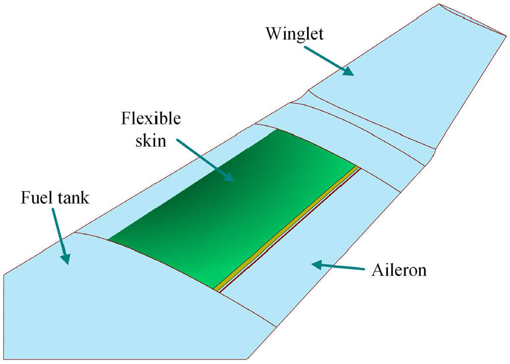
Figure 1. Positioning of the flexible skin on the aircraft wing(Reference Tchatchueng Kammegne, Botez, Mamou, Mebarki, Koreanschi, Sugar Gabor and Grigorie35–Reference Michaud37).

Figure 2. Structural description of the morphing wing model(Reference Tchatchueng Kammegne, Botez, Mamou, Mebarki, Koreanschi, Sugar Gabor and Grigorie35, Reference Michaud37).
The used actuators were identical and controlled by using a control logic developed in LARCASE laboratory. The first test of the developed control system was realised in LARCASE laboratory on a bench test with no airflow. To validate the aerodynamic results given and predicted by the aerodynamic team working in the project, the integrated experimental model was tested in the NRC wind tunnel in Ottawa, Canada. The aerodynamic optimisation aimed to extend the laminar flow or delay the appearance of flow laminar-to-turbulence transition targeting drag reduction. The wind tunnel considered for the experimental validation is a subsonic wind tunnel used for both academic and industrial purposes.
The present paper discusses the modelling, the design and the control of the four electromechanical actuators used in the morphing mechanism of the flexible skin. In addition, the results of the control system experimental validation are shown. A brief description of the hardware used for the experimental validation is presented as well. The particularity of the developed position controller is that it combines the data obtained from an encoder and from a Linear Variable Differential Transformer (LVDT) with the aim to synchronise the sensors. The loop using the LVDT signal as feedback was designed to realise a compensation of the mechanical plays occurring inside the developed actuators.
2.0 MORPHING WING CONTROL SYSTEM DESIGN
2.1 Project motivation
Due to its multidisciplinary character, the project gathered technical experts from different technical fields, such as mechanical and structural engineering, aerodynamics and computational fluid dynamics, electrical and electronic engineering, engineering instrumentation, software engineering, automation and control engineering, from academic, research and industrial entities. According with the trend in the field, it aimed to enhance the environmental impact of the aeronautical industry among other industry areas such as the transport industry, and fuel or petroleum facilities. The drag is one of the parameters which can be influenced to achieve that goal, as its reduction contributes to an economy in fuel consumption. Here, the drag reduction has been realised through the delaying of the transition region by moving it near the wing trailing edge, thus, extending the laminar flow on the upper surface of the wing for the operating range of flow condition. Therefore, the aerodynamic team of the project developed an optimisation algorithm to find the aerofoil optimum shapes by modifying the local thickness to improve the flow on the upper surface. The optimisation was based on a genetic algorithm coupled with the Xfoil software; an algorithm developed by the aerodynamic team(Reference Koreanschi, Sugar and Botez38). The objective function was constructed based on the desired goal to influence the flow on the wing’s upper surface with the purpose to minimise the drag and to delay the laminar-to-turbulent flow transition region for a more stable boundary layer. The optimisation procedure was applied for several flow conditions obtained by combining different Mach numbers (M), angles of attack ( $\alpha $) and aileron deflection angles (
 $\delta $). In this way, the parameters that established the control conditions for the actuators used to morph the flexible skin were the speed, the Reynolds number, the angle-of-attack and the aileron deflection angle(Reference Tchatchueng Kammegne, Botez, Mamou, Mebarki, Koreanschi, Sugar Gabor and Grigorie35, Reference Tchatchueng Kammegne, Botez and Grigorie36).
The optimised flexible skin mounted on the wing was deformed by the mean of four miniature electrical actuators, which can work independently, while the up-and-down deflection of the aileron attached on the wing was realised by an electrical actuator linked to the aileron by using a lever arm. The aerodynamic optimisation of the aerofoil shape provided the displacement values for a pair of actuators, while the displacements for the second pair of actuators were calculated as a linear dependence. Therefore, the genetic optimisation of the wing aerofoil provided the vertical displacements of the four morphing actuators in each optimised flow case (dY  ${}_{\textrm{1opt}}$, dY
  ${}_{\textrm{2opt}}$, dY
  ${}_{\textrm{3opt}}$, dY
  ${}_{\textrm{4opt}}$), generating in this way a database with the needed actuators displacements for different flight conditions. These stored displacements were further used as desired values (reference displacements) for the control system of the morphing wing(Reference Tchatchueng Kammegne, Botez, Mamou, Mebarki, Koreanschi, Sugar Gabor and Grigorie35, Reference Tchatchueng Kammegne, Botez and Grigorie36).
2.2 Experimental setup of the morphing wing model
Having in mind that all four morphing wing actuators are identical, the system designed to control one of them was used in the same configuration for all four. For a given flow condition, the control system commanded the actuators until their linear displacements equalled the reference displacements, which means that the actual vertical positions of the flexible skin at the level of the four actuation points became the same with the desired actuation displacements provided by the aerodynamic optimisation algorithm. The feedback signals from the actuators, in terms of linear displacements, were provided by the LVDTs attached to each of them, and simultaneously, by the encoders integrated inside the motors equipping the actuators, in terms of the rotor angular position. As a practice, to evaluate the aerodynamic gain brought through morphing, the data provided by some Kulite pressure sensors fixed on the morphing skin were used. A Real-Time (RT) Target technology from National Instruments helped to develop a system that interfaced the remote computer with the controlled experimental model(Reference Tchatchueng Kammegne, Botez and Grigorie36, Reference Tchatchueng Kammegne, Grigorie and Botez39).
The hardware component of the morphing wing experimental model included (Fig. 3): (1) a PXIe chassis, used to install the modules and the PXIe controller; (2) a real-time controller (PXIe-8135), with a high-bandwidth PXI Express embedded controller with up to 8 GB/s system and 4 GB/s slot bandwidth, and a 2.3 GHz quad-core Intel Core i7-3610QE processor; (3) four NI PXIe-4330 simultaneous input modules providing integrated data acquisition and signal conditioning for bridge-based sensors; (4) a SCXI chassis, used with a SCXI module connecting the LVDT sensors; (5) a CANopen box extension, with 14 ports wired in parallel to connect multiple devices to NI CAN interfaces; (6) four Power amplifiers, connected to the electrical motors equipping the actuators through controllable outputs; (7) two Programmable power supplies Aim-TTi CPX400DP.

Figure 3. Hardware component for the experimental model.
The microcontroller attached to the amplifier included a control loop with adjustable coefficients. All power amplifier parameters could be accessed through the object dictionary, bringing more flexibility for the user. Figure 4 shows the connection diagram of the drive. The architecture of this drive allows the user to test experimentally any linear controller for the motor by programming the coefficients of the integrated control loop. Moreover, the data sheet of the drive provides various formulas to realise a conversion of the control gains resulted from the design procedures into gains specific to the hardware.

Figure 4. A schema of the drive connection diagram.
2.3 Mathematical modelling of the controlled morphing actuators
To design the morphing wing actuators control system, a prior modelling of the actuators was performed. Each of the four actuators used to morph the flexible skin included in its architecture a brushless direct current (BLDC) motor produced by Maxon Motor Company, a trapezoidal screw, a gearbox system, a nut and a gearing system. The four actuators were designed and manufactured in our laboratory at ETS in Montreal and used identical motors and gearbox.
For an easiest modelling, the BLDC motor could be approximated with enough precision by a linear direct motor. The driver of the motor realises a conversion of the voltage command u(t) into a motor torque. The level of this controlled torque is established depending by the necessary torque to move the load by overcoming of any friction. Therefore, the next dynamic equation can be written as:
 \begin{equation}J({\rm d}w/{\rm d}t)+Bw=T_{e} -T_{L} ;\label{eqn1}\end{equation}
w is the motor angular speed [rad/s], J is the total inertial of the system [Kg $\cdot\textit{m}{}^{2}$], B is the friction coefficient [N
 $\cdot$m/(rad/s)], T
  ${}_{e}$ is the motor torque [N
 $\cdot$m] and T
  ${}_{L}$ is the load torque [N
 $\cdot$m]. The equation relating to the angular speed of the motor with the angular position of its output shaft is:
 \begin{equation}w={\rm d}\theta /{\rm d}t.\label{eqn2}\end{equation}
On the other hand, the torque constant k  ${}_{t}$ ([N
 $\cdot$m/A]) reflects the direct proportionality dependence between the mechanics of the motor, characterised by the desired shaft torque, and the electrics of the motor, characterised by the motor current i:
 \begin{equation}T_{e} =k_{t} i.\label{eqn3}\end{equation}
Therefore, from Equations (1) to (3), it can be demonstrated that:
 \begin{equation}J\, \ddot{\theta }+B\, \dot{\theta }=k_{t} i-T_{L}.\label{eqn4}\end{equation}
In addition, the equation modelling the electrical part of the motor is expressed as follows:
 \begin{equation}u=L({\rm d}i/{\rm d}t)+Ri+e;\label{eqn5}\end{equation}
u is the motor voltage [V], R the motor resistance [ $\Omega $], L the motor inductance [H] and e the back electromotive force (EMF) [V]. From the previous equations and considering the linear dependence between the back EMF and the motor angular speed,
  $e\,{=}\,k_{e}\cdot\textit{w}$, it results:
 \begin{equation}W({\rm s})/U({\rm s})=k_{t} /(LJ\cdot {\rm s}^{2} +RJ\cdot {\rm s}+k_{e} k_{t} );\label{eqn6}\end{equation}
k  ${}_{e}$ is the angular speed constant [revolution/min/V]. In the design of the control system for the morphing wing actuators, a MATLAB/Simulink modelling was performed. In this concern, as a part of this general MATLAB/Simulink scheme, the motor model resulted as in Fig. 5. The first transfer function in the left part of Fig. 5 characterises the electrical part of the motor, while the second transfer function characterises its mechanics.

Figure 5. The motor MATLAB/Simulink simplified model.
2.4 Design of the actuation control system
In order to morph the wing, each of the four actuators should be controllable powered. In this way, by connecting the embedded motors to the proper driver, the power is provided by using a controlled voltage. Due to the fact that the actuation system includes four similar motors and four similar gearboxes, the control system was valid for all four actuators. The architecture of the designed control system in the exposed variant here was based on three loops, one for the torque control and the other two for the position control based on position feedback signals provided by different sensors: (1) the output of an encoder in the first loop; (2) the output of an LVDT in the second loop. Having in mind the facilities provided by the motor’s drivers, both the torque controller and the encoder-based controller were implemented inside it. On the other hand, the LVDT-based control loop beneficiating by the real-time system facilities allowing its independent programming and experimental testing. A schematic representation of the morphing wing control system based on this strategy is shown in Fig. 6.

Figure 6. Control loops.
As it was already specified, the miniature actuators used to morph the wing were designed and manufactured in LARCASE according to the specificity of our application. Having in mind that the morphing wing model was based on the dimensions of a scaled part of a wing for a real aircraft and was designed and experimentally realised to satisfy the constraints imposed by the aeronautical industry applications, some mechanical plays were considered inside the actuators to avoid their blockage under different wing bending situations. Actually, the structural team of the project realised a 1g structural static test to evaluate the integration of the actuators inside the wing structure and its structural integrity (Fig. 7). Therefore, the reason to add in the control architecture of the loop based on the LVDT signals was to compensate these mechanical plays inside the actuators when are controlled theirs positions, and to don’t alter in this way the aerodynamic performance of the wing when is morphed in various flow conditions.

Figure 7. The wing on the bench test during 1g structural static test.
In the next subsections of the paper are presented the design procedures for the control loops associated to the torque and to the actuators position.
2.4.1 Torque controller design
The design of the torque-associated controller is strictly related to the electrical behaviour of the motor. The transfer function related to this part is characterised by the next expression:
 \begin{equation}G_{e} ({\rm s})=\frac{1}{L{\rm s}+R} =\frac{1/R}{(L/R){\rm \; s}+1},\label{eqn7}\end{equation}
which, with the notation,
 \begin{equation}\tau _{e} =L/R,\label{eqn8}\end{equation}
can be rewritten as
 \begin{equation}G_{e} ({\rm s})=\frac{1/R}{\tau _{e} {\rm \; s}+1} =\frac{1/R}{1+\frac{{\rm s}}{{\rm 1/}\tau _{e} } } ;\label{eqn9}\end{equation}
 $\tau $
 ${}_{e}$ is the motor electrical time constant.
On the other hand, according to Equation (3), the target to control the torque (mechanical variable) can be accomplished by using a controlled electrical variable i.e. the electrical current. A Proportional Integral (PI) controller was used for the current, which conducted to the MATLAB/Simulink model in Fig. 8 for the system with controlled torque. Choosing the transfer function of the current controller below
 \begin{equation}G_{i} ({\rm s})=K_{pt} +\frac{K_{it} }{{\rm s}} =\frac{K_{it} }{{\rm s}} \left[{\rm 1}+\frac{{\rm s}}{K_{it} /K_{pt} } \right]\!,\label{eqn10}\end{equation}
the transfer function for the open loop of the system with controlled torque resulted as follows:
 \begin{equation}G_{io} ({\rm s})=G_{i} ({\rm s}){\rm \; }G_{e} ({\rm s})=\frac{K_{it} }{{\rm s}} \left[1+\frac{{\rm s}}{K_{it} /K_{pt} } \right]\frac{1/R}{1+\frac{{\rm s}}{{\rm 1/}\tau _{{\rm e}} } } {\rm ;}\label{eqn11}\end{equation}
where K  ${}_{pt}$ and K
  ${}_{it}$ are the proportional and the integral gains in torque controller, respectively.

Figure 8. System with torque control.
Literature provides many techniques to tune this kind of controller. For our system, the pole-zero cancellation method has been applied(Reference Abe, Zaitsu, Obata, Shoyama, Ninomiya and Yurkevich40). As a consequence, the zero of the current controller was chosen to cancel the pole of the electrical part of the motor transfer function, such that
 \begin{equation}K_{it} /K_{pt} ={\rm 1/\tau }_{e} .\label{eqn12}\end{equation}
Therefore,
 \begin{equation}K_{pt} ={\rm \tau }_{e} \cdot K_{it} =\frac{L}{R} \cdot K_{it},\label{eqn13}\end{equation}
and the transfer function in Equation (11) becomes
 \begin{equation}G_{io} ({\rm s})=(K_{it} /{\rm s)}\cdot (1/R),\label{eqn14}\end{equation}
which, in the frequency domain, leads to
 \begin{equation}\left|G_{io} ( j\omega )\right|=\sqrt{K_{it}^{2} /[R^{2} ( j\omega )^{2} ]} =K_{it} /(R\omega ).\label{eqn15}\end{equation}
 $\omega $ is the pulsation,
  $\omega =2\pi \textit{f}$ (f is the frequency). Rewriting Equation (15) yields
 \begin{equation}\left|G_{io} ( j\omega )\right|_{dB} =20\log _{10} (K_{it} )-20\log _{10} (\omega R),\label{eqn16}\end{equation}
which, at the crossover frequency f  ${}_{s}$, is null. Therefore,
 \begin{equation}20\log _{10} (K_{it} )-20\log _{10} (\omega _{s} \, R)=0,\,\label{eqn17}\end{equation}
and
 \begin{equation}K_{it} =\omega _{s} R;\label{eqn18}\end{equation}
with  $\omega _{s} =2\pi f_{s}.$ It results,
 \begin{equation}\begin{array}{l} {K_{it} =2\pi 1000\, s^{-1} \cdot 3.43\, \Omega =21551.33\, \Omega s^{-1},} \\{K_{pt} =\frac{1.87e-3\, H}{3.43\, \Omega } \cdot 21551.33\, \Omega s^{-1} =11.74\, Hs^{-1}.} \end{array}\label{eqn19}\end{equation}
As it was previously mentioned, the data sheet of the drive provides various formulas to realise a conversion of the control gains resulted from the design procedures into gains specific to the hardware. Therefore,
 \begin{equation}\begin{array}{l} {K_{P...SI} =3.91e-3\, K_{P...EPOS2},\, } \\ {K_{I...SI} =3.910\, \frac{\Omega }{s} K_{I...EPOS2},} \end{array}\label{eqn20}\end{equation}
and the coefficients to be implemented for the current controller parameters result with the values
 \begin{equation}\begin{array}{l} {K_{P...EPOS2} =\frac{11.74}{3.91e-3} =3002.6,} \\ {K_{I...EPOS2} =\frac{21551.33}{3.910} =5512.} \end{array}\label{eqn21}\end{equation}
2.4.1.1 Design of the position control system
Encoder-based position control loop Having in mind that the innermost loop had to be faster than the outer loop (see Fig. 6), then the control loop for the current has been simplified and conducted to the equivalent MATLAB/Simulink model from Fig. 9. According to the actuators mathematical model previously established, the mechanical part is characterised by the next transfer function:
 \begin{equation}G_{m} ({\rm s})=\frac{1}{J{\rm s}+B} \cdot \frac{1}{{\rm s}} =\frac{1/B}{(J/B)\cdot {\rm s}+{\rm 1}} \cdot \frac{1}{{\rm s}}.\label{eqn22}\end{equation}
Considering the mechanical time constant of the motor with the expression  $\tau _{m}=J/B$, Equation (22) becomes
 \begin{equation}G_{m} ({\rm s})=\frac{1/B}{\tau _{m} \cdot {\rm s}+1} \cdot \frac{1}{{\rm s}} =\frac{1/B}{1+\frac{{\rm s}}{{\rm 1/}\tau _{m} } } \cdot \frac{1}{{\rm s}}.\label{eqn23}\end{equation}
As can be observed from Fig. 9, a proportional-derivative (PD) controller has been chosen for the encoder-based position controller; its transfer function can be written under the form
 \begin{equation}G_{p} ({\rm s})=K_{pp} +K_{dp} \cdot {\rm s}=K_{pp} \cdot \left({\rm 1}+\frac{{\rm s}}{K_{pp} /K_{dp} } \right)\! .\label{eqn24}\end{equation}
Therefore, the transfer function for the open loop of the system in Fig. 9 is obtained as
 \begin{equation}G_{po} ({\rm s})=G_{p} (s)\cdot G_{m} (t)\cdot k_{t} =k_{t} K_{pp} \cdot \left({\rm 1}+\frac{{\rm s}}{K_{pp} /K_{dp} } \right)\cdot \frac{1/B}{1+\frac{{\rm s}}{{\rm 1/}\tau _{m} } } \cdot \frac{1}{{\rm s}} ;\label{eqn25}\end{equation}
where K  ${}_{pp}$ and K
  ${}_{dp}$ are the proportional and the derivative gains in position controller, respectively.

Figure 9. Control of the position based on the encoder signal.
Using the pole-zero cancellation method(Reference Abe, Zaitsu, Obata, Shoyama, Ninomiya and Yurkevich40), Equation (25) yields
 \begin{equation}K_{pp} =\frac{{\rm \tau }_{m} }{K_{dp} } =\frac{J}{BK_{dp} },\label{eqn26}\end{equation}
and the transfer function G  ${}_{po}$(s) becomes
 \begin{equation}G_{po} ({\rm s})=k_{t} \cdot \frac{K_{pp} }{{\rm s}} \cdot \frac{1}{B},\label{eqn27}\end{equation}
which, in frequency domain, leads to
 \begin{equation}\left|G_{po} ( j\omega )\right|=\sqrt{K_{pp}^{2} k_{t}^{2} /[B^{2} ( j\omega )^{2} ]} =K_{pp} k_{t} /(B\omega ).\label{eqn28}\end{equation}
 $\omega $ is the pulsation,
  $\omega =2\pi \textit{f} \,(\textit{f}$ - the frequency). Similar with the previous designed controller, at the crossover frequency
  $f_{p}$, we have
 \begin{equation}\left|G_{po} ( j\omega )\right|_{dB} =0,\label{eqn29}\end{equation}
i.e.
 \begin{equation}20\log _{10} (K_{ip} k_{t} )-20\log _{10} (\omega _{p} \, B)=0;\label{eqn30}\end{equation}
with  $\omega _{p} =2\pi f_{p}.$ Therefore,
 \begin{equation}\begin{array}{l} {K_{pp} =\dfrac{\omega _{p} B}{k_{t} } =\dfrac{628\, {\rm rad/s}\cdot 3.8e-6\, {\rm Nm/(rad/s)}}{24.1e-3\, {\rm Nm/A}} =0.099\, {\rm A,}} \\\\[-5pt] {K_{dp} =\dfrac{J}{B} \cdot K_{ip} =\dfrac{0.099\, {\rm A}\cdot 35.3e-7{\rm Kg}\cdot {\rm m}^{{\rm 2}} }{3.8e-6\, {\rm Nm/(rad/s)}} =0.0919\, {\rm As}.} \end{array}\label{eqn31}\end{equation}
For a repeated step signal as a reference position, the numerical simulation results for the designed position controller based on the encoder signal as feedback are shown in Fig. 10.

Figure 10. Numerical simulation for the position control system which uses the encoder signal as feedback.
2.4.1.2 LVDT-based position control loop
A particular element of the proposed control system for the actuators position would be the use of two parallel loops based on the feedback signals provided by the two different sensors (an encoder and an LVDT). The loop using the LVDT signal as feedback was designed to realise a compensation of the mechanical plays inside the developed actuators. Therefore, by cancelling these plays, the feedback signals are the same with the real displacements of the flexible skin in the four actuation points. To synchronise the control loops, in the control system, near the position set point and the position provided by the LVDT, was added, as a third input, the position provided by the encoder. The MATLAB/Simulink model implementing the control structure is shown in Fig. 11.

Figure 11. Actuators position control based on the LVDT signals as feedback.
The position control-based LVDT signals were implemented using fuzzy logic techniques, which usually offers tools to experts to interpret the human knowledge into real-world applications, which enriches the design of the systems based on conventional methods with engineering expertise. In many applications, it is difficult to obtain a reliable and rigorous mathematical model of systems; thus, the fuzzy logic technique could be used to overcome this kind of situation. Fuzzy logic is also recommended when a linear controller shows some limitations; fuzzy controllers belong to the category of non-linear controllers and are based on rules. Mainly, a basic fuzzy logic controller has the structure shown in Fig. 12, including a fuzzification interface, a fuzzy inference engine, a knowledge base (rules implementation) and a defuzzification interface(Reference Grigorie and Botez41–Reference Zadeh45).

Figure 12. Fuzzy logic controller architecture.
The first step is the fuzzification. At this stage, the fuzzifier converts, scales and transforms the crisped input into linguistic variables using the appropriated membership functions. At the second step, the control logic used by the designed controller is required under the form of rules set. The linguistic values for the output linguistic variables are obtained after a knowledge base is called by the interference engine. The last step is the defuzzification, which converts the fuzzy data into a crisp number based on the output membership functions(Reference Grigorie and Botez41–Reference Zadeh45).
For our application, a fuzzy proportional (FP) controller with one input and one output was developed. The controller input was considered the actuation error, calculated taking into account the LVDT signal as feedback, while its output was set to be the control signal. For the controller input eleven membership functions (mf) ( $A_{1}^{1} \div A_{1}^{11} $) were chosen and uniformly distributed in the [−10, 10] interval, considered as universe of discourse. Also, based on the same interval as universe of discourse, eleven membership functions were established for the controller output. For both input and output, the used linguistic terms were: Zero (Z), Positive Very Small (PVS), Positive Small (PS), Positive Medium (PM), Positive Large (PL), Positive Very Large (PVL), Negative Very Small (NVS), Negative Small (NS), Negative Medium (NM), Negative Large (NL) and Negative Very Large (NL). The membership functions of the input were chosen with a triangular shape characterised by Equation 32(Reference Grigorie, Popov, Botez, Mamou and Mébarki22):
 \begin{equation}f_{\Delta } (x;a,b,c)=\left\{\begin{array}{l}{0,\, \, \, \, \, \, \, \, \, \, \, {\rm if}\, \, \, x{\le} a,} \\[3pt]{\frac{x-a}{b-a},\, \, \, \ \ {\rm if}\, \, \, a{\lt}x{\lt}b,} \\[3pt]{\frac{c-x}{c-b},\, \, \, \ \ {\rm if}\, \, \, b{\le} x{\lt}c,} \\[3pt]{0,\, \, \, \, \, \, \, \, \, \, \, {\rm if}\, \, \, c\le x,} \end{array}\right. =\max \!\left[\min \!\left(\frac{x-a}{b-a},\frac{c-x}{c-b} \right)\!,\, \, 0\right]\!,\label{eqn32}\end{equation}
where x is the independent variable on the universe, a and c position the triangle base and b gives its peak(Reference Grigorie, Popov, Botez, Mamou and Mébarki22). Table 1 exposes the values of these parameters for each of the eleven membership functions of the input, while Fig. 13 depicts the allures of these membership functions.
Table 1 Values for the parameters for each of the eleven membership functions of the input


Figure 13. Membership functions of the input.
In the rules definition, a Sugeno fuzzy model has been used(Reference Mahfouf, Linkens and Kandiah44). For our controller, with a single input and a single output, such a model can be written as follows:
 \begin{equation}`{\rm if}\quad (x_{1} \ \ {\rm is}\ \ A)\ \ {\rm then}\quad y=f(x_{1})\text{'}\label{eqn33}\end{equation}
where A is fuzzy set in the antecedent, and  $\textit{y}=\textit{f}(\textit{x}_{1}$) is a crisp function in the consequent by polynomial type. When the polynomial function f is by a first order, then we have a first-order Sugeno fuzzy model, and when f is a constant, then we have a zero-order Sugeno fuzzy model. Applied for our controller, with a single input and a single output, a first-order Sugeno fuzzy model with N rules can be expressed as(Reference Grigorie and Botez41, Reference Mahfouf, Linkens and Kandiah44):
 \begin{equation}\begin{array}{c} {{\rm Rule}\, \, {\rm 1:}\, \, \, \, {\rm If}\, \, x_{1} \, \, {\rm is}\, \, A_{1}^{1},\, \, \, \, {\rm then}\, \, y^{1} (x_{1} )=b_{0}^{1} +a_{1}^{1} x_{1},} \\ {\cdots } \\ {{\rm Rule}\, \, i{\rm :}\, \, \, \, {\rm If}\, \, x_{1} \, \, {\rm is}\, \, A_{1}^{i},\, \, \, \, {\rm then}\, \, y^{ i} (x_{1} )=b_{0}^{i} +a_{1}^{i} x_{1},} \\ {\cdots } \\ {{\rm Rule}\, \, N{\rm :}\, \, \, \, {\rm If}\, \, x_{1} \, \, {\rm is}\, \, A_{1}^{N},\, \, \, \, {\rm then}\, \, y^{N} (x_{1} )=b_{0}^{N} +a_{1}^{N} x_{1},} \end{array}\label{eqn34}\end{equation}
where x  ${}_{1}$ is the input variable,
  ${y^{ i} \, (i=\overline{1,N})}$ is the crisp function in the consequent by the form of a first-order polynomial and
  ${A_{1}^{i} \, (i=\overline{1,N})}$ are the membership functions of input variable. The coefficients
  ${a_{1}^{i} \, (i=\overline{1,N})}$ are parameters of the linear function, and
  ${b_{0}^{i} \, \, (i=\overline{1,N})}$ denote scalar offsets.
For any input x, if the singleton fuzzifier, the product operation fuzzy implication for fuzzy inference and the centre average defuzzifier are applied (Sugeno type), then the crisp control action results under the form of a weighted average (Fig. 14 a)(Reference Grigorie and Botez26)
 \begin{equation}y=\left(\sum _{i=1}^{N}w^{ i} ({\it x})y^{ i} \right)/\left(\sum _{i=1}^{N}w^{ i} ({\it x}) \right)\!,\, \, \, \, w^{ i} ({\it x})=A_{1}^{i} (x_{1} ).\label{eqn35}\end{equation}

Figure 14. Output of the fuzzy model and the obtained inference rules.
For the output membership functions, constant values were chosen ( $\textrm{NVL}=-10, \textrm{NL}\,{=}\,{-}\,8,\ \textrm{NM}=-6,\ \textrm{NS}=-4,\ \textrm{NVS}=-2,\ \textrm{Z}=0,\ \textrm{PVS}=2,\ \textrm{PS}=4,\ \textrm{PM}=6,\ \textrm{PL}=8$,
  $\textrm{PVL}=10$); the parameters
  ${a_{1}^{i} \, (i=\overline{1,N})}$ of the linear functions from Equation (34) were considered with null values. Based on the established membership functions, a set containing eleven rules was built (
 $N=11$) (Fig. 14 b).
In a first validation test of the controller, some numerical simulations were performed. The responses of the position controller, which used the LVDT signal as feedback for various repeated step signals as reference positions, are presented in Fig. 15.

Figure 15. Numerical simulation of the position control system based on the LVDT feedback.
The numerical results revealed that the rise time of the controlled system is about 1.6 seconds, and the steady-state errors are null for all responses. On the other hand, the allures of the graphical characteristics can be easily observed that there is no overshoot whatever the rotation sense of the motor. The absence of the steady-state error created the premises to fulfil the requirements of the aerodynamic team, which asked for an absolute maximum value of this error lower than 0.1 mm at the level of the four actuation points on the experimental model.
3.0 EXPERIMENTAL TESTING AND EVALUATION OF THE CONTROL SYSTEM
The experimental testing of the developed control system was performed in two independent steps: (1) bench testing in the LARCASE laboratory with wind off; (2) wind-tunnel testing at NRC. The control was used in the same form for all four morphing actuators placed inside the wing.
3.1 Bench test results
The experimental bench test with different components is displayed in Fig. 16 (the lower face of the wing is removed). Two steps in the implementation of the full control system were performed here: (1) The innermost controller and the encoder feedback-based position controller were directly programmed in the power drive by using the object dictionary; (2) The LVDT feedback-based position controller required a Simulink compilation to obtain the equivalent C code, which was further loaded on the real-time system by using an ethernet cable.

Figure 16. Morphing wing-tip experimental model during bench testing.
The signal conditioner of the LVDT was used to generate a drive signal for the LVDT, to process its output and to send it to the control system. The position of the motor provided by the encoder fixed at the level of its stator was accessed by the RT Target through a CANopen bus and further sent to the controller, which controlled the position based on the LVDT signal as feedback.
In the first phase of the bench testing, all of the four miniaturised actuators were individually controlled by using various signals independent over time from one actuator to another. At one step, similarly with the numerical simulations, successive steps signals of various amplitudes were applied at the input of the actuators as desired displacements signals. Figure 17 shows the experimental results obtained during this test for one of the actuators, under the flexible skin load but with no wind blowing; the graphical characteristics also include the numerical simulation results for the same inputs. Both from the graphical characteristics and from the acquired numerical values, it was observed that the position obtained from the experimental measurements follows closely the curve of the position resulted from the numerical simulation, with a small deviation in the transient phase, which is not a drawback for the developed system.

Figure 17. Bench test experimental validation of the designed controller.
In the second phase of the bench testing, the control results were evaluated for all optimised flow cases by using the database of the numerically obtained vertical displacements (dY  ${}_{\textrm{1opt}}$, dY
  ${}_{\textrm{2opt}}$, dY
  ${}_{\textrm{3opt}}$, dY
  ${}_{\textrm{4opt}}$) of the four morphing actuators. Therefore, for each optimised flow case, the inputs of the system controlling the four actuators were the optimised values of the vertical displacements in the four actuation points, dY
  ${}_{\textrm{1opt}}$, dY
  ${}_{\textrm{2opt}}$, dY
  ${}_{\textrm{3opt}}$, dY
  ${}_{\textrm{4opt}}$, characterising the optimised aerofoil obtained for that case. For all optimised aerofoil cases, the numerical values of the real vertical displacements in the four actuation points, dY
  ${}_{\textrm{1real}}$, dY
  ${}_{\textrm{2real}}$, dY
  ${}_{\textrm{3real}}$, dY
  ${}_{\textrm{4real}}$, revealed that the developed and experimentally implemented control system for the morphing wing actuators worked well in the tested conditions, where the morphing wing-tip experimental model was not aerodynamically loaded. Therefore, as the effect aerodynamic loads on the flexible skin deformation was expected to be negligible, the experimental model was cleared for testing in the wind tunnel.
3.2 Results obtained during wind-tunnel testing of the morphing wing-tip model
To test the morphing wing-tip experimental model in the presence of aerodynamic loads, the NRC 2 m $\,{\times}\,3$ m atmospheric closed-circuit subsonic wind tunnel was used. About 97 flight cases were tested based on the combinations between 19 values for the angles of attack, varied from
  $-3$ degree to
  $+3$ degree, three values for the Mach numbers (0.15, 0.2 and 0.25) and 13 values for the aileron deflection angles, between
  $-6$ degrees and
  $+6$ degrees. Figure 18 exposes the installation of the morphing wing experimental model in the NRC wind tunnel during the tests: the left picture is a view from the leading-edge side, while the right picture is a view from the trailing-edge side. The experimental model was mounted in a vertical position, the different incidence angles being obtained by rotating the model around a vertical axis.

Figure 18. The installation of the morphing wing experimental model in the NRC wind tunnel.
For each tested flight case, three runs have been performed in the wind tunnel: (1) the first run as a tare run of the wind tunnel; (2) the second run to evaluate the reference (un-morphed) aerofoil; (3) the third run to evaluate the morphed aerofoil under the form of optimised aerofoil corresponding to the tested flight case. The developed control system has been used during the third run corresponding to each tested flight case, and it controlled the morphing actuators inside the wing in order to achieve the optimised vertical displacements (i.e. the optimised aerofoil) corresponding to that flight case. The optimised vertical displacements (dY  ${}_{\textrm{1opt}}$, dY
  ${}_{\textrm{2opt}}$, dY
  ${}_{\textrm{3opt}}$, dY
  ${}_{\textrm{4opt}}$) for each tested flight case were used as desired displacements and taken from the database generated by the aerodynamic team of the project.
Two methodologies have been used to evaluate the aerodynamic gain of the morphing wing technology on the experimental model. These were successively applied for the un-morphed and for the morphed configurations of the experimental model and after that a comparative analysis has been performed. The first one supposed the estimation of the laminar-to-turbulent transition point position in a very small area of the wing, based on pressure data acquired from 32 Kulite pressure sensors arranged on two closes chord lines (40% of the wing span and 41.7% of the wing span), while the second one allowed us to capture the laminar-to-turbulent transition area over the entire upper surface of the wing by using the infrared (IR) thermography technique for the flow visualisation.
For each wind-tunnel run, important data for the monitoring of the morphing wing experimental model were acquired and stored: the pressure data provided by the 32 Kulite pressure sensors at a rate of 20Kz, the flexible skin displacements in the four actuation points, the actuators speeds and the electrical currents that crossed them. In each tested flight case, the data were acquired for the tare run, for the reference (un-morphed) aerofoil run and for the morphed aerofoil run. Because, during the evaluation of the aerodynamic gain, the fixed target was to compare the results obtained for the un-morphed and for the morphed configurations, but also, because of big quantity of data needed to be stored, no data were acquired during the transition between the un-morphed and the morphed configurations. On the other hand, starting from the pressure sensors signals, a real-time visualisation of the transition point position, based on the Fast Fourier Transform (FFT) comparative analysis between the detection channels, has been performed; the pressure coefficients obtained from the experimental data were used to validate the optimised wing aerofoil for each tested flow case. The real-time data processing and visualisation related to the transition point position, in the second and third runs of the each wind-tunnel tested flight case, validated the optimised wing shapes obtained by the aerodynamic team by using the numerical optimisation procedure based on the genetic algorithm. Subsequently, a recorded pressure data post processing step was performed to obtain the FFT spectral decomposition, the standard deviation (stocktickerSTD) values for each pressure channel and the position of the laminar-to-turbulent transition.
The actuation results for the flow case 43 (Mach = 0.15,  $\alpha =2^\circ$,
  $\delta =0^\circ$) presented in Fig. 19 show a very good behaviour of the designed control system for all four actuators in the presence of the aerodynamic load and wind-tunnel vibrations. Similar results were obtained for all tested cases, and very small values were noticed of the overshoot or its absence, rise times under 3 seconds and a very low level of the steady-state errors located well below the 0.1 mm, a value allowed by the aerodynamic team.

Figure 19. The actuation results for the flow case 43 (Mach = 0.15,  $\alpha =2^{\circ}$,
  $\delta =0^{\circ}$).
Figure 20 illustrates the STD of the pressure data recorded during the testing of the flow case 43 (Mach = 0.15,  $\alpha =2^\circ$,
  $\delta =0^\circ$), evaluating the transition position for reference and morphed aerofoils. The Kulite sensors were positioned on the flexible skin between 28% and 68% of the chord. A higher standard deviation picked up by a Kulite among the others suggests that the sensed pressure signal was induced by turbulence, which started somewhere between that Kulite sensor and the previous one. Similar effects can be observed at the level of the FFT evaluated for all pressure sensors. A detached FFT curve indicates that a turbulent flow over the respective pressure sensor occurred. The resolution for the evaluation of the position for laminar-to-turbulent transition is directly determined by the density of the pressure sensors evaluating the flow characteristics. Figures 21 and 22 depict the FFT evaluation results, respectively, for un-morphed aerofoil and morphed aerofoil for flow condition case 43 (Mach = 0.15,
  $\alpha =2^\circ$,
  $\delta =0^\circ$). For a better visualisation of the transition location, the 32 Kulite sensors FFTs were represented in 4 independent windows in groups of 8 consecutive sensors starting from the leading edge. Figures 21 and 22 provide also a centralised representation of the FFTs for all 32 sensors for an easiest observation of the FFTs curves detachment.

Figure 20. Standard deviations of the pressure data recorded in the flow case 43 (Mach = 0.15,  $\alpha =2^{\circ}$,
  $\delta =0^{\circ}$).

Figure 21. FFT results for the un-morphed aerofoil in the flow case 43 (Mach = 0.15,  $\alpha =2^{\circ}$,
  $\delta =0^{\circ}$).

Figure 22. FFT results for the morphed aerofoil in the flow case 43 (Mach = 0.15,  $\alpha =2^{\circ}$,
  $\delta =0^{\circ}$).
The results presented in Fig. 23 show that the transition for the un-morphed aerofoil started on pressure sensor #10 positioned at 42.45% of the chord and has a maximum value on pressure sensor #13 positioned at 45.16% of the chord. The morphed aerofoil improved the flow over the wing, the transition point being detected on pressure sensor #16 positioned at 50.79% of the chord.

Figure 23. IR caption of the transition region for the flow case 43 (Mach = 0.15,  $\alpha =2^{\circ}$,
  $\delta =0^{\circ}$).
From the FFT point of view, the graphical curves in Fig. 21 for the un-morphed aerofoil also suggest that the transition started on pressure sensor #10, and the maximum influenced FFT curve is associated to the sensor on channel #13, confirming in this way the STD results. From the fifth picture of the figure, it can be easily observed that the first detached FFT curve is associated with pressure sensor #9.
From Fig. 22, corresponding to FFT curves for the morphed aerofoil in the flow case 43, can be observed that the turbulence is maximum on sensor #16, while the FFT curves detachment start around the sensors on channels #14 and #15. The conclusion sustains the allure obtained for the STD curve in the second picture of Fig. 20.
To capture the laminar-to-turbulent transition area over the entire upper surface of the wing, flow visualisation using the IR thermography technique has been realised. To improve the quality of the IR captions, high emissivity black paint has been used to coat the wing parts viewed with the infrared camera: the flexible skin on the upper surface, the leading edge and the aileron. To avoid the contamination of pressure sensors, but also the negative influence on the pressure readings from the 32 Kulite sensors, the area on the upper wing surface where the two sensor lines were mounted was not coated with the paint. The measurement of the monitored surface temperature has been performed with a Jenoptik VarioCAM camera, operating at a frame rate of 30 Hz at  $640 \times 480$ IR pixel resolution and equipped with
  $60^{\circ}$ lens to visualise the transition region over the whole upper surface of the morphing wing model(Reference Mebarki, Mamou and Genest46–Reference Koreanschi, Sugar Gabor, Acotto, Brianchon, Portier, Botez, Mamou and Mebarki49).
Figure 23 presents the results of the IR visualisation of the wing model’s upper surface transition for the flow case 43 (Mach = 0.15,  $\alpha =2^{\circ}$,
  $\delta =0^{\circ}$) for un-morphed aerofoil (left figure) and for morphed aerofoil (right figure), respectively. The black line from Fig. 23 represents the average transition line on the upper surface being estimated in the following steps. At each span-wise station, an automatic detection was performed of the temperature gradients due to the transition. The temperature gradient method allowed the detection of the transition onset (upstream dotted white line in the figures) as well as the established turbulent boundary layer (downstream dotted lines). The mean transition location front is the span-wise average of the upstream and downstream fronts. From the figure, it is observed that the transition location is a function of the chord-wise position. The two dashed white lines represent the estimated extent of the transition region, determined as a function of the chord-wise temperature gradient existing between laminar and turbulent regimes. The dot on the mean transition location line at 0.4 from the wing span (y/c
 $\,=\,$0.4) represents the estimate of the transition point position starting from the Kulite pressure data and evaluated in the span-wise section obtained as a mean of the two Kulite sensors lines; this mean span-wise section was positioned at 0.612 m from the root section i.e. at 40% of the model span.
It can be observed that the IR visualisations validate the STD and FFT estimated positions of the transition points on the Kulite pressure sensors area, for reference (un-morphed) aerofoil, but also for the morphed aerofoil corresponding to the exposed flow case. For the un-morphed aerofoil, the mean value for the transition position for the whole wing was estimated to be at approximately 47%( $\pm$3%) of the chord (47.29%(
 $\pm$3%)), while for the morphed aerofoil the value was approximately 50%(
 $\pm$3%) of the chord (50.42%(
 $\pm$3%)). Therefore, according to the IR measurements, the extension of the laminar region for this flow case was of about 3.13%(
 $\pm$3%) of chord.
Starting from the Kulite pressure sensors data, the transition point position evaluation for the un-morphed aerofoil conducted at the value 43.62% of the chord when the STD method was used, and at the value 37.54% of the chord when the FFT method was used i.e. a mean value of 40.58% of the chord. On the other hand, for the morphed aerofoil, the obtained results were 50.79% of the chord for the STD method and 42.45% of the chord for the FFT method i.e. a mean value of 46.62% of the chord. As a consequence, the evaluated gains related to the extension of the laminar region for this flow case were 7.17% of the chord for the STD method, 4.91% of the chord for the FFT method and 6.04% of the chord for the mean values mixing the two methods.
4.0 CONCLUSIONS
The paper presented the modelling, the design and the control of the miniaturised electromechanical actuators used to morph the flexible skin in a new multidisciplinary morphing wing research project. The results obtained during the control system evaluation in bench tests and wind-tunnel tests were analysed and discussed. A scaled part of a wing for a real aircraft was used as a reference to design and manufacture the experimental model. Also, a flexible skin made of composite fibre materials was mounted on the upper surface of the wing. Spars, ribs, stringers and an aileron were integral parts of the wing model. The actuation system included four similar miniature electromechanical actuators placed directly at the actuation points on two actuation lines, which were designed in-house and manufactured according to the specificity of the developed application. The feedback signals from the actuators in terms of linear displacements are provided by the LVDTs attached to each of them, and simultaneously, by the encoders integrated in the motors driving the actuators, in terms of the rotor angular position. The use of the LVDT-based control loop as the second control loop in position is aimed at the compensation of the mechanical plays inside the actuators, from the position control point of view, and at the avoidance of the morphing wing aerodynamic performance alteration in various flow conditions. The evaluation of the project gain from the aerodynamic point of view has been made by using the data provided by a number of Kulite pressure sensors monitoring the airflow on the wing upper surface. On the other hand, a RT Target technology from National Instruments has been used to develop an interface system between the remote computer and the controlled morphing wing model.
After the mathematical modelling of the actuators, the associated control system architecture was established, and the design of the included control loops was performed. The pole-zero cancellation method has been used to tune the torque controller and the position controller based on the encoder data, while the position control based on the LVDT data implementation used the fuzzy logic technology. In a first validation test of the control system, some numerical simulations were performed. The experimental validation of the developed control system was performed in two independent steps: (1) bench testing in the LARCASE laboratory at ETS with no airflow; (2) wind-tunnel testing at NRC. The control was used in the same form for all four morphing actuators placed inside the wing.
Experimental model bench testing was performed in two steps: (1) individual control of the four actuators by using various signals independent over time from one actuator to another; (2) simultaneous control of the four actuators for all optimised flow cases, using as inputs the vertical displacements in the four actuation points (dY ${}_{\textrm{1opt}}$, dY
 ${}_{\textrm{2opt}}$, dY
 ${}_{\textrm{3opt}}$, dY
 ${}_{\textrm{4opt}}$) characterising the optimised aerofoils. For all tested optimised aerofoil cases, the numerical values of the real vertical displacements in the four actuation points (dY
 ${}_{\textrm{1real}}$, dY
 ${}_{\textrm{2real}}$, dY
 ${}_{\textrm{3real}}$, dY
 ${}_{\textrm{4real}}$) revealed that the developed and experimentally implemented control system worked well in the tested conditions, where the wing model was not aerodynamically loaded.
During the wind-tunnel testing in the NRC 2 m $\,{\times}\,$3 m atmospheric closed-circuit subsonic wind tunnel, 97 flight cases were evaluated and the main signals such as the pressure data provided by the 32 Kulite pressure sensors, the flexible skin displacements in the four actuation points, the actuators speeds and the electrical currents that crossed them were acquired and stored. On the other hand, starting from the pressure sensors signals, a real-time visualisation of the transition point position, based on the FFT comparative analysis between the detection channels, has been performed; the pressure coefficients obtained from the experimental data were used to validate the optimised wing aerofoil for each tested flow case. Subsequently, a recorded pressure data post-processing step was performed to obtain the FFT spectral decomposition, the STD values for each pressure channel and the position of the laminar-to-turbulent transition. The tests of the un-morphed and morphed aerofoils demonstrated the validity of the morphing wing concept in terms of the transition location improvement due to morphing, and therefore, the functionality of the wing experimental model and of the designed control system.
To capture and to confirm in real time the laminar-to-turbulent transition area over the entire upper surface of the wing, flow visualisation by using the IR thermography technique has been realised. The IR results served as a tangible reference in validating the STD- and FFT-estimated positions of the transition points.
5.0 DIRECTIONS OF FUTURE WORK
The work presented in this paper was developed numerically and was further validated through experiments. In this work, in case of actuator failure, the linear position sensor could be damaged. It could be interesting therefore to redesign the integration of the actuator with a linear position sensor in the screw axis as a safety measure for the possible damage of this sensor. Because of the irregular deformation of the skin due to the actuators’ punctual positions, it will be chosen to place an array of actuators instead. In a previous project realised by our team, smart material actuators were placed on the morphing wing skin. The control architecture, integrated within the voltage amplifier, would allow linear control for the torque and position based on the encoder as a feedback signal. The voltage amplifier would be designed in the current (torque) mode, and a different control algorithm would be developed for the position control based on the encoder. This newly designed controller could be deployed in the real-time system. The morphing wing equipped with the aileron developed in this project for an already existing regional aircraft would need to be integrated and developed on the aircraft. Wind-tunnel and flight test should be performed to analyse the benefits of installing this concept on the regional aircraft. There will be the need to obtain up to 10% in fuel consumption reduction.
ACKNOWLEDGEMENTS
The authors would like to thank the Thales Avionics team (Mr Philippe Molaret, Mr Bernard Bloiuin and Mr Xavier Louis) and the Bombardier Aerospace team (Mr Patrick Germain and Mr Fassi Kafyeke) for their help and financial support. We would also like to thank the Consortium for Research and Innovation in Aerospace in Quebec (CRIAQ) and the National Sciences and Engineering Research Council (NSERC) for their funding of the CRIAQ MDO 505 project. Thanks are also due to Master Student Yvan Tondji for providing support in the post-processing of the data.


