NOMENCLATURE
- p, q, r
-
roll, pitch and yaw angular rates
- m, g
-
mass of the aircraft, gravity acceleration
- V
-
velocity
- MV , Mq
-
aerodynamic pitch moment derivatives with respect to V and q
- TV , DV , LV
-
thrust, aerodynamic drag-and-lift derivatives with respect to V
- Ix , Iy , Iz , Izx
-
inertia moments and inertia product
- *, Δ
-
equilibrium point and its deviation
Greek Symbol
- α, β
-
angle-of-attack and sideslip angle
- ϕ, θ, ψ
-
roll or bank, pitch and yaw angles
- δ T , δ e , δ a , δ r
-
throttle, elevator, aileron and rudder deflections
- L δ e , D δ e
-
aerodynamic lift-and-drag derivatives with respect to δ e
-
L
α, D
α,
 $L_{\dot{\alpha }}$
-
aerodynamic lift-and-drag derivatives with respect to
$\alpha , \dot{\alpha }$
- L β, Lp , Lr
-
aerodynamic roll moment derivatives with respect to β, p, r
- N β, Np , Nr
-
aerodynamic yaw moment derivatives with respect to β, p, r
- N δ a , N δ r
-
aerodynamic yaw moment derivatives with respect to δ a , δ r
-
M
α,
$M_{\dot{\alpha }}$
, M
δ
e
-
aerodynamic pitch moment derivatives with respect to α,
$\dot{\alpha }$
and δ
e
- T, T δ T
-
engine thrust and its derivative with respect to δ T
- Y β, Yp , Yr , Y δ a , Y δ r
-
side force derivatives with respect to β, p, r, δ a , δ r


1.0 INTRODUCTION
The Unmanned Aerial Vehicles (UAVs) receive more and more attention in the field of civil and military due to their light weight, small size, high mobility, strong adaptability and so on. In 1917, Britain successfully developed the world’s first UAV(Reference Qin and Wang1). UAVs have been used in war since the 1960s in the Vietnam War(Reference Zou, He and He2). In the Gulf War in 1991, many countries employed a variety of UAVs to conduct reconnaissance, assess the battle damage and search and rescue people. For the national economy, UAVs are used for geodesy, meteorological observation, artificial rainfall and so on. The technology of UAVs has been relatively mature. In spite of this, a single UAV may be influenced by large flight resistance and is difficult to complete the complex tasks. For the purpose of reducing the flight resistance and making as full as possible the use of each UAV, scientific researchers imitate some abilities of biology and put forward the concept of formation flight of UAVs, which enables UAVs to complete the formation flight, military mapping, co-operative combat missions and so on(Reference Pu, Zhen and Xia3,Reference Bennet, McInnes, Suzuki and Uchiyama4) . Such a UAVs formation is capable of accomplishing tasks which a single UAV either fulfills with difficulty, such as accurate determination of the location for an object, or fails to accomplish altogether, such as mapping of inaccessible caves or dense rain forest, assessment of real-time environmental processes, or wildlife monitoring. Furthermore, compared with a single UAV, UAVs formation is not only able to complete more tasks, but also able to reduce the time of executing various activities and to increase the quality of collected data. For these applications, several key technical problems should be addressed, such as co-operative path planning(Reference Madhavan, Antonios, Rafal and Brian5,Reference Zhen, Gao, Zheng and Jiang6) , co-operative mission planning(Reference Gao, Zhen and Gong7), formation relative navigation(Reference Zhen, Hao, Gao and Jiang8), formation control(Reference Wei9) and collision avoidance(Reference Lorenz and Walter10). Under such research background, it is of great importance to research formation flight control and its engineering applications.
After a collection of UAVs enter the designated area, they begin to form formation. In the UAVs formation, the key problems are formation keeping and control. Generally, the formation structure in the process of formation flight remains the same, which depends on the formation flight control strategy. The formation flight control strategy is divided into two aspects. One is the information interaction between a collection of UAVs, the other is the formation control algorithm. At present, specific formation strategies mainly include: leader-follower formation strategy, behaviour-based formation strategy, virtual structure formation strategy and artificial potential field formation strategy. Correspondingly, many control algorithms based on UAVs formation flight control problem have been derived, such as: H∞ control(Reference Renan and Karl11); proportion integration differentiation control(Reference Zuo and Hu12); feedback linearisation(Reference Mohammad and Mohammad13); linear quadratic control(Reference Giulietti, Innocenti, Napolitano and Pollini14,Reference Rinaldi, Chiesa and Quagliotti15) ; fuzzy control(Reference Abbas and Wu16) and adaptive control (Reference Semsar17). However, among the methods above, most adopt the corresponding control methods based on the known dynamic models, while the adaptive control used in Ref. 17 does not consider the leader dynamic uncertainty.
In order to make a group of UAVs keep a certain formation structure, there should exist information interactions among them. In the information interactions control strategies, generally speaking, there are centralised control strategy, distributed control strategy and decentralised control strategy. For the centralised control strategy, each UAV needs to interact its own position, velocity, attitude and moving targets with all UAVs in the formation(Reference Zhu18). Namely, each UAV should know the whole information of the formation. The centralised control strategy is of the best control effect but it depends on mass information interactions, which rely on complex control algorithms and may lead to conflict. For the distributed control strategy, each UAV needs to interact its own position, velocity, attitude and moving targets with the adjacent UAVs(Reference Joongbo, Chaeik and Youdan19). Although the control effect is relatively poor, it depends on less information interactions and decreases the computing load. Therefore, the distributed control strategy relies on a relatively simple control system. For the decentralised control strategy, each UAV only needs to keep itself and the fixed points with the relative relations in the formation and does not communicate with others(Reference Lechevin20). As there is almost no information interactions among UAVs, it greatly decreases the computing load and depends on the simplest structure. However, the control effect is the worst. In conclusion, the control effect of the distributed control strategy is worse than the centralised control strategy, but its control structure is simple and reliable. Additionally, the distributed control strategy depends on less information interactions and is more likely to avoid information conflict, while the decentralised control strategy may lead to the collision among UAVs. Therefore, this paper adopts the distributed control strategy to solve the problem of information interactions and collision at the same time.
For many cases in the UAVs formation, the model parameters of both the leader and followers are unknown; it is difficult to control the formation flight by a fixed controller. Hence, it is necessary to design adaptive control laws to update parameters of the model in time. Adaptive control is a control methodology capable of effectively accommodating large system parametric and structural uncertainties under the matching conditions(Reference Sang21). In the case of unknown model parameters, adaptive control will make the system still achieve the desired properties(Reference Tao22). A majority of existing research is focused on the leader-follower formation strategy assuming that the parameters of followers are uncertain, while not much effort has been made in the literature towards considering the leader and the follower dynamic uncertainties at the same time.
Therefore, in this paper, we focus on the distributed leader-follower UAVs formation flight control problem, based on a multivariable Model Reference Adaptive Control (MRAC) strategy. Different from the results in the literature, the main contributions of this paper are as follows.
-
1) For the purpose of accomplishing the distributed leader-follower UAVs formation flight control, a state feedback state tracking multivariable MRAC strategy is presented. Being different from the fixed control in Ref. 12, this control algorithm is based on the unknown parameters. The stability and tracking performance of the formation flight system can be achieved applying the multivariable MRAC algorithm.
-
2) For the distributed leader-follower UAVs formation flight control problem with parametric uncertainties, a novel multivariable MRAC scheme is proposed. In the real UAVs formation flight environment, it is difficult to get accurate UAVs dynamic parameters. Both the parametric uncertainties of the leader and the followers are considered. This problem has not been addressed in the literature. The stability and tracking performance of the formation flight system is analysed in detail, to guarantee the wing UAVs will track the lead UAV asymptotically.
The remainder of this paper is organised as follows. In Section 2, we consider the parametric uncertainties for both the leader and the followers, and then establish dynamic models of UAVs in formation flight. The algebraic graph theory which denotes the information interactions among UAVs will be discussed in this section as well. In Section 3, we develop a new adaptive control scheme for the distributed leader-follower formation flight control problem with uncertain parameters for both the leader and the followers. In Section 4, we present the simulation results of UAVs formation flight to illustrate the effectiveness of the proposed multivariable MRAC method. Finally, in Section 5 we discuss some conclusions in this paper and the potential future work.
2.0 FLIGHT CONTROL PROBLEM OF UAVs FORMATION
In this section, based on the dynamic model of UAVs, the distributed leader-following system models with the parameter uncertainties are established, a multivariable MRAC scheme for multiple UAVs formation is designed, and the control objective is described, in order to help illustrate the problem formulation.
2.1 UAVs dynamic model
A linearised UAVs model can be obtained based on small pertubation principle(Reference Zhen, Wang and Kang23)
 $$\begin{equation}
E\dot{X}=AX+BU,
\end{equation}$$
$$\begin{equation}
E\dot{X}=AX+BU,
\end{equation}$$
where E, A and B are Jacobian matrices, X = [V β α θ p q r] T .
If E is non-singular, then Equation (1) can be written in the form of standard linear state equation
 $$\begin{equation}
\dot{X}=\widetilde{A}X+\widetilde{B}U
\end{equation}$$
$$\begin{equation}
\dot{X}=\widetilde{A}X+\widetilde{B}U
\end{equation}$$
Generally, the linear model of Equation (2) is decoupled into a longitudinal model and a lateral model.
 $$\begin{equation}
\dot{X}_{lon}=A_{lon}X_{lon}+B_{lon}U_{lon}
\end{equation}$$
$$\begin{equation}
\dot{X}_{lon}=A_{lon}X_{lon}+B_{lon}U_{lon}
\end{equation}$$
 $$\begin{equation}
\dot{X}_{lat}=A_{lat}X_{lat}+B_{lat}U_{lat},
\end{equation}$$
$$\begin{equation}
\dot{X}_{lat}=A_{lat}X_{lat}+B_{lat}U_{lat},
\end{equation}$$
where Xlon = [ΔV, Δα, Δq, Δθ] T , Ulon = [Δδ e , Δδ T ] T , Xlat = [Δβ, Δp, Δr] T , Ulat = [Δδ a , Δδ r ] T , and
 $$\begin{eqnarray*}
A_{lon}\!\!=\!\!{ \left[ \begin{array}{c@{\hspace*{4pt}}c@{\hspace*{4pt}}c@{\hspace*{4pt}}c}\frac{T_V\cos \alpha ^*-D_V}{m} \!\!&\!\! -\frac{T^*\sin \alpha ^*+D_{\alpha }-mg\cos {{\mu }^*}}{m} \!\!&\!\! 0 \!\!&\!\! -g\cos {{\mu }^*}\\[3pt]
-\frac{T_V\sin \alpha ^*+L_V}{L_{\dot{\alpha }}+mV^*} \!\!&\!\! -\frac{T^*\cos \alpha ^*+L_{\alpha }-mg\sin {{\mu }^*}}{L_{\dot{\alpha }}+mV^*} \!\!&\!\! -\frac{L_q-mV^*}{L_{\dot{\alpha }}+mV^*} \!\!&\!\! -\frac{mg\sin {{\mu }^*}}{L_{\dot{\alpha }}+mV^*} \\[4pt]
\frac{M_V}{I_y}\!-\!M_{\dot{\alpha }}\frac{T_V\sin \alpha ^*+L_V}{I_y(L_{\dot{\alpha }}+mV^*)} \!&\! \frac{M_\alpha }{I_y}\!-\!M_{\dot{\alpha }} \frac{T^*\cos \alpha ^*+L_{\alpha }-mg\cos {{\mu }^*}}{I_y(L_{\dot{\alpha }}+mV^*)} \!&\! \frac{M_q}{I_y}\!-\!M_{\dot{\alpha }}\frac{L_q-mV^*}{I_y(L_{\dot{\alpha }}+mV^*)} \!&\! -\frac{M_{\dot{\alpha }}mg\sin {{\mu }^*}}{I_y(L_{\dot{\alpha }}+mV^*)}\\[2pt]
0 \!\!&\!\! 0 \!\!&\!\! 1 \!\!&\!\! 0
\end{array} \right]}
\end{eqnarray*}$$
$$\begin{eqnarray*}
A_{lon}\!\!=\!\!{ \left[ \begin{array}{c@{\hspace*{4pt}}c@{\hspace*{4pt}}c@{\hspace*{4pt}}c}\frac{T_V\cos \alpha ^*-D_V}{m} \!\!&\!\! -\frac{T^*\sin \alpha ^*+D_{\alpha }-mg\cos {{\mu }^*}}{m} \!\!&\!\! 0 \!\!&\!\! -g\cos {{\mu }^*}\\[3pt]
-\frac{T_V\sin \alpha ^*+L_V}{L_{\dot{\alpha }}+mV^*} \!\!&\!\! -\frac{T^*\cos \alpha ^*+L_{\alpha }-mg\sin {{\mu }^*}}{L_{\dot{\alpha }}+mV^*} \!\!&\!\! -\frac{L_q-mV^*}{L_{\dot{\alpha }}+mV^*} \!\!&\!\! -\frac{mg\sin {{\mu }^*}}{L_{\dot{\alpha }}+mV^*} \\[4pt]
\frac{M_V}{I_y}\!-\!M_{\dot{\alpha }}\frac{T_V\sin \alpha ^*+L_V}{I_y(L_{\dot{\alpha }}+mV^*)} \!&\! \frac{M_\alpha }{I_y}\!-\!M_{\dot{\alpha }} \frac{T^*\cos \alpha ^*+L_{\alpha }-mg\cos {{\mu }^*}}{I_y(L_{\dot{\alpha }}+mV^*)} \!&\! \frac{M_q}{I_y}\!-\!M_{\dot{\alpha }}\frac{L_q-mV^*}{I_y(L_{\dot{\alpha }}+mV^*)} \!&\! -\frac{M_{\dot{\alpha }}mg\sin {{\mu }^*}}{I_y(L_{\dot{\alpha }}+mV^*)}\\[2pt]
0 \!\!&\!\! 0 \!\!&\!\! 1 \!\!&\!\! 0
\end{array} \right]}
\end{eqnarray*}$$
 $$\begin{eqnarray*}
B_{lon}= \left[ \begin{array}{c@{\hspace*{4pt}}c}-\frac{D_{\delta _e}}{m} & \frac{T_{\delta _T}\cos \alpha ^*}{m} \\[4pt]
-\frac{L_{\delta _e}}{L_{\dot{\alpha }}+mV^*} & -\frac{T_{\delta _T}\sin \alpha ^*}{L_{\dot{\alpha }}+mV^*}\\[4pt]
\frac{M_{\delta _e}}{I_y}-\frac{M_{\dot{\alpha }}L_{\delta _e}}{I_y(L_{\dot{\alpha }}+mV^*)} & -\frac{M_{\dot{\alpha }}T_{\delta _T}\sin \alpha ^*}{I_y(L_{\dot{\alpha }}+mV^*)}\\[2pt]
0 & 0 \end{array} \right]
\end{eqnarray*}$$
$$\begin{eqnarray*}
B_{lon}= \left[ \begin{array}{c@{\hspace*{4pt}}c}-\frac{D_{\delta _e}}{m} & \frac{T_{\delta _T}\cos \alpha ^*}{m} \\[4pt]
-\frac{L_{\delta _e}}{L_{\dot{\alpha }}+mV^*} & -\frac{T_{\delta _T}\sin \alpha ^*}{L_{\dot{\alpha }}+mV^*}\\[4pt]
\frac{M_{\delta _e}}{I_y}-\frac{M_{\dot{\alpha }}L_{\delta _e}}{I_y(L_{\dot{\alpha }}+mV^*)} & -\frac{M_{\dot{\alpha }}T_{\delta _T}\sin \alpha ^*}{I_y(L_{\dot{\alpha }}+mV^*)}\\[2pt]
0 & 0 \end{array} \right]
\end{eqnarray*}$$
 $$\begin{eqnarray*}
A_{lat}= \left[ \begin{array}{c@{\quad}c@{\quad}c}\frac{Y_\beta }{mV^*} & \sin \alpha ^*+\frac{Y_p}{mV^*} & \frac{Y_r}{mV^*}-\cos \alpha ^*\\[5pt]
\frac{I_zL_\beta +I_{zx}N_\beta }{I_xI_z-I_{zx}^2} & \frac{I_zL_p+I_{zx}N_p}{I_xI_z-I_{zx}^2} & \frac{I_zL_r+I_{zx}N_r}{I_xI_z-I_{zx}^2} \\[5pt]
\frac{I_{zx}L_\beta +I_xN_\beta }{I_xI_z-I_{zx}^2} & \frac{I_{zx}L_p+I_xN_p}{I_xI_z-I_{zx}^2} & \frac{I_{zx}L_r+I_xN_r}{I_xI_z-I_{zx}^2}
\end{array} \right]
\end{eqnarray*}$$
$$\begin{eqnarray*}
A_{lat}= \left[ \begin{array}{c@{\quad}c@{\quad}c}\frac{Y_\beta }{mV^*} & \sin \alpha ^*+\frac{Y_p}{mV^*} & \frac{Y_r}{mV^*}-\cos \alpha ^*\\[5pt]
\frac{I_zL_\beta +I_{zx}N_\beta }{I_xI_z-I_{zx}^2} & \frac{I_zL_p+I_{zx}N_p}{I_xI_z-I_{zx}^2} & \frac{I_zL_r+I_{zx}N_r}{I_xI_z-I_{zx}^2} \\[5pt]
\frac{I_{zx}L_\beta +I_xN_\beta }{I_xI_z-I_{zx}^2} & \frac{I_{zx}L_p+I_xN_p}{I_xI_z-I_{zx}^2} & \frac{I_{zx}L_r+I_xN_r}{I_xI_z-I_{zx}^2}
\end{array} \right]
\end{eqnarray*}$$
 $$\begin{eqnarray*}
B_{lat}= \left[ \begin{array}{c@{\hspace*{4pt}}c}\frac{Y_{\delta _a}}{mV^*} & \frac{Y_{\delta _r}}{mV^*} \\[5pt]
\frac{I_zL_{\delta _a}+I_{zx}N_{\delta _a}}{I_xI_z-I_{zx}^2} & \frac{I_zL_{\delta _r}+I_{zx}N_{\delta _r}}{I_xI_z-I_{zx}^2}\\[5pt]
\frac{I_{zx}L_{\delta _a}+I_xN_{\delta _a}}{I_xI_z-I_{zx}^2} & \frac{I_{zx}L_{\delta _r}+I_xN_{\delta _r}}{I_xI_z-I_{zx}^2}
\end{array} \right]
\end{eqnarray*}$$
$$\begin{eqnarray*}
B_{lat}= \left[ \begin{array}{c@{\hspace*{4pt}}c}\frac{Y_{\delta _a}}{mV^*} & \frac{Y_{\delta _r}}{mV^*} \\[5pt]
\frac{I_zL_{\delta _a}+I_{zx}N_{\delta _a}}{I_xI_z-I_{zx}^2} & \frac{I_zL_{\delta _r}+I_{zx}N_{\delta _r}}{I_xI_z-I_{zx}^2}\\[5pt]
\frac{I_{zx}L_{\delta _a}+I_xN_{\delta _a}}{I_xI_z-I_{zx}^2} & \frac{I_{zx}L_{\delta _r}+I_xN_{\delta _r}}{I_xI_z-I_{zx}^2}
\end{array} \right]
\end{eqnarray*}$$
with Alon and Blon , Alat and Blat being unknown model parameters.
In general, we design the longitudinal and lateral controllers separately, based on the same control method. Therefore, in order to design the control law conveniently, we establish a generalised dynamic model of the UAVs to design the control law. The unified longitudinal and lateral state-space model can be expressed as
 $$\begin{equation}
\dot{x}=Ax+Bu
\end{equation}$$
$$\begin{equation}
\dot{x}=Ax+Bu
\end{equation}$$
Here, for designing the longitudinal controller, x denotes Xlon , A denotes Alon , B denotes Blon and u denotes Ulon , and Alon and Blon have unknown model parameters. For designing the lateral controller, x denotes Xlat , A denotes Alat , B denotes Blat and u denotes Ulat , and Alat and Blat have unknown model parameters.
2.2 Formation flight control problem of distributed leader-following system with uncertain parameters
The formation flight problem of UAVs can be described as the leader-follower formation problem, where the lead UAV is the leader and the wing UAVs are the followers. The dynamic model of UAVs is in the form of the leader-following system including one leader and N followers.
Dynamic Model of Leader-Following System. The dynamic of the N followers and one leader can be represented as
 $$\begin{equation}
\dot{x}_i(t)=A_ix_i(t)+B_iu_i(t),\quad i=1,\dots ,N
\end{equation}$$
$$\begin{equation}
\dot{x}_i(t)=A_ix_i(t)+B_iu_i(t),\quad i=1,\dots ,N
\end{equation}$$
 $$\begin{equation}
\dot{x}_0(t)=A_{0}x_0(t)+B_{0}u_0(t),
\end{equation}$$
$$\begin{equation}
\dot{x}_0(t)=A_{0}x_0(t)+B_{0}u_0(t),
\end{equation}$$
where all Ai and Bi are the unknown parameter matrices of the followers. A 0 is an unknown constant and stable matrix, and B 0 is an unknown constant matrix. xi (t) ∈ Rn is the state of the ith follower, ui (t) ∈ R pi is the control input, x 0(t) ∈ Rn is the state of the leader, and u 0(t) ∈ Rm is the bounded input.
Remark 1. Different from the existing MRAC method with parametric uncertainties only for the followers, the proposed multivariable MRAC method can be applied to the system with uncertain parameters (A 0, B 0) for the leader at the same time.
Remark 2. In the distributed leader-following UAVs formation flight control system, x 0(t) denotes the states of the lead UAV, and u 0(t) represents the control input of the lead UAV. Therefore, they are bounded and available for measurement.
Control objective. The control objective is to design a distributed adaptive control scheme for each follower to make all followers track the leader on states asymptotically, i.e. lim t → ∞(xi (t) − x 0(t)) = 0, i = 1, . . ., N.
Given the distributed leader-follower UAVs formation flight control problem with uncertain parameters, an advanced control method is indispensable. MRAC is a popular control methodology capable of dealing with the uncertain systems to ensure desired control performance, accommodating the system parametric, structural, and environmental uncertainties, component failures, and external disturbances(Reference Guo, Tao and Liu24). Therefore, in this paper, a multivariable MRAC method is presented to solve the distributed leader-follower UAVs formation flight control problem.
2.3 MRAC framework
An MRAC scheme is designed for the distributed UAVs formation flight control problem, whose schematic diagram is shown in Fig. 1. The control system is mainly composed of the flight control system and the controlled object. The proposed MRAC scheme has an adaptation capacity to deal with parameter uncertainties for both the leader and the followers.

Figure 1. An MRAC scheme for multiple UAVs formation.

Figure 2. Formation I: Interactions among one leader and two followers.

Figure 3. Formation II: Interactions among one leader and two followers.

Figure 4. Formation III: Interactions among one leader and two followers.

Figure 5. Formation IV: Interactions among one leader and two followers.
2.4 Algebraic graph theory
For the problem of distributed multiple UAVs formation, the interactions among N + 1 UAVs are similar to a graph with directions. While in mathematics the algebraic graph theory is based on the graphs, which describes the topological relations among individuals. Therefore, the knowledge of algebraic graph theory is introduced to the design of UAVs formation flight control to denote the communication topology relations among UAVs.
A directed graph can be represented as G = (V, E), where V is a set of vertices and E⊆V × V is a set of directed edges. A vertex denotes a UAV and the directed edge (vj , vi ) denotes that the follower vi can obtain the information from the follower vj including both the state and input information, but not vice versa. Under such circumstances, vj is one of the neighbors of vi . Define a neighborhood set Ni = {vj ∈ V: (vj , vi ) ∈ E} for i = 1, . . ., N. v 0 denotes the leader in the leader-following system. A directed path is composed of a sequence of ordered edges of the form (v i1, v i2), (v i2, v i3), . . . in a directed graph.
In order to make the UAVs formation realised, we give two assumptions on the interaction graphs.
Assumption 1. For each UAV vi , there exists at least one directed path (v 0, v 1), (v 1, v 2), . . ., (v i − 1, vi ) which starts from the leader and ends at the follower vi .
Assumption 2. Directed path G has no loop and no multiple arcs (arcs with same starting and ending nodes).
Assumption 1 and 2 are necessary for the leader-following system to achieve the control objectives effectively. The leader-following system we established is simple but can deal well with the distributed UAVs formation flight control problem.
3.0 ADAPTIVE FORMATION FLIGHT CONTROL DESIGN
In order to meet the control objectives, we will solve the distributed leader-follower UAVs formation flight control problem using the MRAC theory.
3.1 Adaptive control design for formation flight control problem of distributed leader-following system with uncertain parameters
For the multivariable linearised system Equation (6) with unknown system matrices (Ai , Bi ), the control objective is to design bounded state feedback control laws ui (t) to make all the followers’ state xi (t) bounded and track the leader’s state x 0(t) asymptotically, i.e. lim t → ∞(xi (t) − x 0(t)) = 0.
To meet the control objective, we make some assumptions first.
Assumption 3. There exist two parameter matrices K*1i ∈ R n × pi and K*4i ∈ R pi × pi for each follower, which satisfy:
 $$\begin{equation}
A_e=A_i+B_iK_{1i}^{*T},\quad B_e=B_iK_{4i}^*,
\end{equation}$$
$$\begin{equation}
A_e=A_i+B_iK_{1i}^{*T},\quad B_e=B_iK_{4i}^*,
\end{equation}$$
where Ae ∈ R n × n is a stable and known matrix and Be ∈ R n × p is a known matrix;
Assumption 4. There exist two parameter matrices K*2i0 ∈ R pi × m and K*3i0 ∈ R n × pi such that
 $$\begin{equation}
A_0=A_i+B_iK_{3i0}^{*T},\quad B_0=B_iK_{2i0}^*
\end{equation}$$
$$\begin{equation}
A_0=A_i+B_iK_{3i0}^{*T},\quad B_0=B_iK_{2i0}^*
\end{equation}$$
if the leader is one of the neighbors of the follower vi (i.e. (v 0, vi ) ∈ E). Otherwise, if (v 0, vi )∉E,
 $$\begin{equation}
A_j=A_i+B_iK_{3ij}^{*T},\quad B_j=B_iK_{2ij}^*
\end{equation}$$
$$\begin{equation}
A_j=A_i+B_iK_{3ij}^{*T},\quad B_j=B_iK_{2ij}^*
\end{equation}$$
should be satisfied for some K*2ij ∈ R pi × pj and K*3ij ∈ R n × pi for each pair of (vj , vi ) ∈ E(j ≠ 0).
Assumption 5. There is a known matrix Si ∈ R pi × pi for each follower such that K*4i Si is symmetric and positive definite: Ms = K*4i Si = (K*4i Si ) T > 0.
Assumption 3 and Assumption 4 are the following plant-model state matching conditions. Assumption 4 means that the N followers are classified into two groups. Each follower in the first group can get the information from the leader directly, thus for each (v 0, vi ), there exist two matrices K*2i0 and K*3i0 satisfying Equation (9). While in the second group, followers have no direct accesses to the leader, then for each (vj , vi ) (j ≠ 0), there exist two matrices K*2ij and K*3ij satisfying Equation (10). In a word, for each directed edges (vj , vi ), there exist a set of corresponding K*2ij and K*3ij (0 ⩽ j ⩽ N) whether vj is the leader or not. Assumption 5 is needed to design the control law.
If the parameters of Ai , Bi , A 0 , B 0 were known, then the above control objective can be met by using the nominal controller
 $$\begin{equation}
u_i^*(t)=\frac{1}{n_i}\sum _{v_j\in N_i}(K_{1i}^{*T}(x_i(t)-x_j(t))+K_{2ij}^*u_j(t)+K_{3ij}^{*T}x_j(t)) ),
\end{equation}$$
$$\begin{equation}
u_i^*(t)=\frac{1}{n_i}\sum _{v_j\in N_i}(K_{1i}^{*T}(x_i(t)-x_j(t))+K_{2ij}^*u_j(t)+K_{3ij}^{*T}x_j(t)) ),
\end{equation}$$
where ni is the total number in the neighborhood set Ni .
Substituting Equation (11) into Equation (6), the ith subsystem (6) becomes
 $$\begin{eqnarray}
\dot{x}_i(t)&=&A_ix_i(t)+\frac{1}{n_i}B_i\sum _{v_j\in N_i}(K_{1i}^{*T}(x_i(t)-x_j(t))+K_{2ij}^*u_j(t)+K_{3ij}^{*T}x_j(t)) \nonumber\\
&=&\frac{1}{n_i}B_i\sum _{v_j\in N_i}(A_e(x_i(t)-x_j(t))+A_jx_j(t)+B_ju_j(t))
\end{eqnarray}$$
$$\begin{eqnarray}
\dot{x}_i(t)&=&A_ix_i(t)+\frac{1}{n_i}B_i\sum _{v_j\in N_i}(K_{1i}^{*T}(x_i(t)-x_j(t))+K_{2ij}^*u_j(t)+K_{3ij}^{*T}x_j(t)) \nonumber\\
&=&\frac{1}{n_i}B_i\sum _{v_j\in N_i}(A_e(x_i(t)-x_j(t))+A_jx_j(t)+B_ju_j(t))
\end{eqnarray}$$
A local tracking error for each UAV is defined as
 $$\begin{equation}
e_i(t)=x_i(t)-\frac{1}{n_i}\sum _{v_j\in N_i}x_j(t),
\end{equation}$$
$$\begin{equation}
e_i(t)=x_i(t)-\frac{1}{n_i}\sum _{v_j\in N_i}x_j(t),
\end{equation}$$
which shows the disagreement between the follower i and the average of its neighbors on states. And a global tracking error for each UAV is xi (t) − x 0(t).
Lemma 1. Ref. 25 If lim t → ∞ ei (t) = 0 holds, then lim t → ∞(xi (t) − x 0(t)) = 0 holds for all i = 1, . . ., N.
Lemma 1 has been demonstrated with detail in Ref. 25; the proof is omitted here. Instead, we give a simple example to describe the relationship between the local tracking error and the global tracking error.
Assuming that there exist three UAVs including one leader and two followers, for this directed graph, there are four possible formation configurations in total.
Formation I: In this case, if the local tracking errors are e 1(t) = x 1(t) − x 0(t) → 0 and e 2(t) = x 2(t) − x 1(t) → 0 as t → ∞, then the global tracking errors x 1(t) − x 0(t) → 0 and x 2(t) − x 0(t) → 0 as t → ∞ are achieved. Particularly, this kind of formation structure is called the basic structure, namely a directed path which starts from the leader and ends at the last follower.
Formation II: In this case, the local tracking errors are e 1(t) = x 1(t) − x 0(t) → 0 and e 2(t) = x 2(t) − x 0(t) → 0 as t → ∞, then the global tracking errors x 1(t) − x 0(t) → 0 and x 2(t) − x 0(t) → 0 as t → ∞ are achieved, obviously.
Formation III: In this case, the local tracking errors are
 $e_1(t)=x_1(t)-\frac{1}{2}x_0(t)-\frac{1}{2}x_2(t)\rightarrow 0$
and e
2(t) = x
2(t) − x
0(t) → 0 as t → ∞, then the global tracking errors x
1(t) − x
0(t) → 0 and x
2(t) − x
0(t) → 0 as t → ∞ are achieved.
$e_1(t)=x_1(t)-\frac{1}{2}x_0(t)-\frac{1}{2}x_2(t)\rightarrow 0$
and e
2(t) = x
2(t) − x
0(t) → 0 as t → ∞, then the global tracking errors x
1(t) − x
0(t) → 0 and x
2(t) − x
0(t) → 0 as t → ∞ are achieved.
Formation IV: This case is similar to Formation III; the global tracking errors x 1(t) − x 0(t) → 0 and x 2(t) − x 0(t) → 0 as t → ∞ are achieved as well.
In the distributed leader-follower UAVs formation flight control problem, the parameters of Ai , Bi , A 0, B 0 are unknown. An adaptive controller is given as
 $$\begin{equation}
u_i(t)=\frac{1}{n_i}\sum _{v_j\in N_i}(K_{1i}(t)^{T}(x_i(t)-x_j(t))+K_{2ij}(t)u_j(t)+K_{3ij}(t)^{T}x_j(t)),
\end{equation}$$
$$\begin{equation}
u_i(t)=\frac{1}{n_i}\sum _{v_j\in N_i}(K_{1i}(t)^{T}(x_i(t)-x_j(t))+K_{2ij}(t)u_j(t)+K_{3ij}(t)^{T}x_j(t)),
\end{equation}$$
where K 1ij (t) , K 2ij (t) and K 3ij (t) are the estimates of K*1i , K*2ij and K*3ij , respectively. (Since for each vj ∈ Ni , the estimates of K*1i are different, thus K 1ij (t) is used to denote the estimates of K*1i ). The design task is to choose adaptive laws to update these estimates so that the control objective is still achievable even if all the parameters are unknown.
To be specific, the adaptive laws to update the control parameters are proposed as(Reference Song25)
 $$\begin{eqnarray}
\dot{K}_{1ij}^T(t) &=& -\frac{1}{n_i}S_i^TB_e^TPe_i(t)(x_i(t)-x_j(t))^T,
\end{eqnarray}$$
$$\begin{eqnarray}
\dot{K}_{1ij}^T(t) &=& -\frac{1}{n_i}S_i^TB_e^TPe_i(t)(x_i(t)-x_j(t))^T,
\end{eqnarray}$$
 $$\begin{eqnarray}
\dot{K}_{2ij}(t) &=& -\frac{1}{n_i}S_i^TB_e^TPe_i(t)u_j^T(t),
\end{eqnarray}$$
$$\begin{eqnarray}
\dot{K}_{2ij}(t) &=& -\frac{1}{n_i}S_i^TB_e^TPe_i(t)u_j^T(t),
\end{eqnarray}$$
 $$\begin{eqnarray}
\dot{K}_{3ij}^T(t) &=& -\frac{1}{n_i}S_i^TB_e^TPe_i(t)x_j^T(t),(v_j\in N_i, i=1,2,\dots ,N),
\end{eqnarray}$$
$$\begin{eqnarray}
\dot{K}_{3ij}^T(t) &=& -\frac{1}{n_i}S_i^TB_e^TPe_i(t)x_j^T(t),(v_j\in N_i, i=1,2,\dots ,N),
\end{eqnarray}$$
where P = PT > 0 satisfies Ae T P + PAe = −Q < 0 for any chosen Q ∈ R n × n being constant and Q = QT > 0. Si ∈ R pi × pi satisfies Assumption 5.
Theorem 1. The adaptive controller, Equation (14), with the adaptive laws, Equation (15)–(17), applied to the plant, Equation (6), guarantees that all closed-loop signals are bounded and all the global tracking errors xi (t) − x 0(t) go to zero as t goes to infinity.
Proof. First of all, substituting Equation (14) into Equation (6), we obtain
 $$\begin{eqnarray}
\dot{x}_i(t)&=&A_ix_i(t)+\frac{1}{n_i}B_i\sum _{v_j\in N_i}(K_{1i}^{T}(x_i(t)-x_j(t))+K_{2ij}u_j(t)+K_{3ij}^{T}x_j(t)) \nonumber\\
&=&\frac{1}{n_i}B_i\sum _{v_j\in N_i}(A_e(x_i(t)-x_j(t))+A_jx_j(t)+B_ju_j(t)) \nonumber\\
&&+\,\frac{1}{n_i}B_e\sum _{v_j\in N_i}(K_{4i}^{*-1}\widetilde{K}_{1ij}^T(t)(x_i(t)-x_j(t))\nonumber\\
&&+\,K_{4i}^{*-1}\widetilde{K}_{2ij}(t)u_j(t)+K_{4i}^{*-1}\widetilde{K}_{3ij}^T(t)x_j(t)),
\end{eqnarray}$$
$$\begin{eqnarray}
\dot{x}_i(t)&=&A_ix_i(t)+\frac{1}{n_i}B_i\sum _{v_j\in N_i}(K_{1i}^{T}(x_i(t)-x_j(t))+K_{2ij}u_j(t)+K_{3ij}^{T}x_j(t)) \nonumber\\
&=&\frac{1}{n_i}B_i\sum _{v_j\in N_i}(A_e(x_i(t)-x_j(t))+A_jx_j(t)+B_ju_j(t)) \nonumber\\
&&+\,\frac{1}{n_i}B_e\sum _{v_j\in N_i}(K_{4i}^{*-1}\widetilde{K}_{1ij}^T(t)(x_i(t)-x_j(t))\nonumber\\
&&+\,K_{4i}^{*-1}\widetilde{K}_{2ij}(t)u_j(t)+K_{4i}^{*-1}\widetilde{K}_{3ij}^T(t)x_j(t)),
\end{eqnarray}$$
and then we derive the adaptive control based on the tracking error equations
 $$\begin{eqnarray}
\dot{e}_i(t)&=&A_e(x_i(t)-\frac{1}{n_i}\sum _{v_j\in N_i}x_j(t))\nonumber\\
&&+\,\frac{1}{n_i}B_eK_{4i}^{*-1}\sum _{v_j\in N_i}(\widetilde{K}_{1ij}^T(t)(x_i(t)-x_j(t))+\widetilde{K}_{2ij}(t)u_j(t)+\widetilde{K}_{3ij}^T(t)x_j(t))\nonumber\\
&=&A_ee_i(t)+\frac{1}{n_i}B_eK_{4i}^{*-1}\sum _{v_j\in N_i}(\widetilde{K}_{1ij}^T(t)(x_i(t)-x_j(t))\nonumber\\
&&+\,\widetilde{K}_{2ij}(t)u_j(t)+\widetilde{K}_{3ij}^T(t)x_j(t)),
\end{eqnarray}$$
$$\begin{eqnarray}
\dot{e}_i(t)&=&A_e(x_i(t)-\frac{1}{n_i}\sum _{v_j\in N_i}x_j(t))\nonumber\\
&&+\,\frac{1}{n_i}B_eK_{4i}^{*-1}\sum _{v_j\in N_i}(\widetilde{K}_{1ij}^T(t)(x_i(t)-x_j(t))+\widetilde{K}_{2ij}(t)u_j(t)+\widetilde{K}_{3ij}^T(t)x_j(t))\nonumber\\
&=&A_ee_i(t)+\frac{1}{n_i}B_eK_{4i}^{*-1}\sum _{v_j\in N_i}(\widetilde{K}_{1ij}^T(t)(x_i(t)-x_j(t))\nonumber\\
&&+\,\widetilde{K}_{2ij}(t)u_j(t)+\widetilde{K}_{3ij}^T(t)x_j(t)),
\end{eqnarray}$$
where
 $\widetilde{K}_{1ij}(t)=K_{1ij}(t)-K_{1i}^*$
,
$\widetilde{K}_{1ij}(t)=K_{1ij}(t)-K_{1i}^*$
,
 $\widetilde{K}_{2ij}(t)=K_{2ij}(t)-K_{2ij}^*$
,
$\widetilde{K}_{2ij}(t)=K_{2ij}(t)-K_{2ij}^*$
,
 $\widetilde{K}_{3ij}(t)=K_{3ij}(t)-K_{3ij}^*$
are parameter errors.
$\widetilde{K}_{3ij}(t)=K_{3ij}(t)-K_{3ij}^*$
are parameter errors.
We choose a positive definite function to analyse the closed-loop system stability as
 $$\begin{equation}
V=\sum _{i=1}^{N}V_i
\end{equation}$$
$$\begin{equation}
V=\sum _{i=1}^{N}V_i
\end{equation}$$
with Vi = V 1i + V 2i , where
 $$\begin{equation}
V_{1i}=e_i^TPe_i
\end{equation}$$
$$\begin{equation}
V_{1i}=e_i^TPe_i
\end{equation}$$
and
 $$\begin{equation}
V_{2i}=\sum _{v_j\in N_i}tr[\widetilde{K}_{1i}M_s^{-1}\widetilde{K}_{1i}^T]+\sum _{v_j\in N_i}tr[\widetilde{K}_{2ij}^TM_s^{-1}\widetilde{K}_{2ij}]+\sum _{v_j\in N_i}tr[\widetilde{K}_{3ij}M_s^{-1}\widetilde{K}_{3ij}^T]
\end{equation}$$
$$\begin{equation}
V_{2i}=\sum _{v_j\in N_i}tr[\widetilde{K}_{1i}M_s^{-1}\widetilde{K}_{1i}^T]+\sum _{v_j\in N_i}tr[\widetilde{K}_{2ij}^TM_s^{-1}\widetilde{K}_{2ij}]+\sum _{v_j\in N_i}tr[\widetilde{K}_{3ij}M_s^{-1}\widetilde{K}_{3ij}^T]
\end{equation}$$
with tr[M] denoting the trace of a square matrix M.
Substituting Equation (19) in Equation (21), we have
 $$\begin{eqnarray}
\dot{V}_{1i}&=&2e_i^T(t)P\dot{e}_i(t)\nonumber\\
&=&e_i^T(t)(PA_e+A_eP)e_i(t)+\frac{2}{n_i}e_i^T(t)PB_eK_{4i}^{*-1}\sum _{v_j\in N_i}\widetilde{K}_{1i}^T(t)(x_i(t)-x_j(t))\nonumber\\[-2pt]
&&+\,\frac{2}{n_i}e_i^T(t)PB_eK_{4i}^{*-1}\sum _{v_j\in N_i}\widetilde{K}_{2ij}(t)u_j(t) +\frac{2}{n_i}e_i^T(t)PB_eK_{4i}^{*-1}\sum _{v_j\in N_i}\widetilde{K}_{3ij}^T(t)x_j(t) \nonumber\\
\end{eqnarray}$$
$$\begin{eqnarray}
\dot{V}_{1i}&=&2e_i^T(t)P\dot{e}_i(t)\nonumber\\
&=&e_i^T(t)(PA_e+A_eP)e_i(t)+\frac{2}{n_i}e_i^T(t)PB_eK_{4i}^{*-1}\sum _{v_j\in N_i}\widetilde{K}_{1i}^T(t)(x_i(t)-x_j(t))\nonumber\\[-2pt]
&&+\,\frac{2}{n_i}e_i^T(t)PB_eK_{4i}^{*-1}\sum _{v_j\in N_i}\widetilde{K}_{2ij}(t)u_j(t) +\frac{2}{n_i}e_i^T(t)PB_eK_{4i}^{*-1}\sum _{v_j\in N_i}\widetilde{K}_{3ij}^T(t)x_j(t) \nonumber\\
\end{eqnarray}$$
Then, compute the time derivative of V 2i
 $$\begin{eqnarray}
\dot{V}_{2i} &=&2\sum _{v_j\in N_i}tr[\widetilde{K}_{1i}(t)M_s^{-1}\dot{\widetilde{K}}_{1i}^T(t)]+2\sum _{v_j\in N_i}tr[\widetilde{K}_{2ij}^T(t)M_s^{-1}\dot{\widetilde{K}}_{2ij}(t)] \nonumber\\
&&+\,2\sum _{v_j\in N_i}tr[\widetilde{K}_{3ij}(t)M_s^{-1}\dot{\widetilde{K}}_{3ij}^T(t)]
\end{eqnarray}$$
$$\begin{eqnarray}
\dot{V}_{2i} &=&2\sum _{v_j\in N_i}tr[\widetilde{K}_{1i}(t)M_s^{-1}\dot{\widetilde{K}}_{1i}^T(t)]+2\sum _{v_j\in N_i}tr[\widetilde{K}_{2ij}^T(t)M_s^{-1}\dot{\widetilde{K}}_{2ij}(t)] \nonumber\\
&&+\,2\sum _{v_j\in N_i}tr[\widetilde{K}_{3ij}(t)M_s^{-1}\dot{\widetilde{K}}_{3ij}^T(t)]
\end{eqnarray}$$
Using the definition Ms = k*4i Si = (k*4i Si ) T > 0 and the properties that tr[M 1 M 2] = tr[M 2 M 1], tr[M 3] = tr[MT 3], we obtain
 $$\begin{eqnarray}
&& e_i^T(t)PB_ek_{4i}^{*-1}\sum _{v_j\in N_i}\widetilde{K}_{1i}^T(t)(x_i(t)-x_j(t)) \nonumber\\
&&\quad =\sum _{v_j\in N_i}tr[e_i^T(t)PB_ek_{4i}^{*-1}\widetilde{K}_{1i}^T(t)(x_i(t)-x_j(t))] \nonumber\\
&&\quad =\sum _{v_j\in N_i}tr[\widetilde{K}_{1i}M_s^{-1}S_i^TB_e^TPe_i(t)(x_i(t)-x_j(t))^T]
\end{eqnarray}$$
$$\begin{eqnarray}
&& e_i^T(t)PB_ek_{4i}^{*-1}\sum _{v_j\in N_i}\widetilde{K}_{1i}^T(t)(x_i(t)-x_j(t)) \nonumber\\
&&\quad =\sum _{v_j\in N_i}tr[e_i^T(t)PB_ek_{4i}^{*-1}\widetilde{K}_{1i}^T(t)(x_i(t)-x_j(t))] \nonumber\\
&&\quad =\sum _{v_j\in N_i}tr[\widetilde{K}_{1i}M_s^{-1}S_i^TB_e^TPe_i(t)(x_i(t)-x_j(t))^T]
\end{eqnarray}$$
 $$\begin{eqnarray}
&& e_i^T(t)PB_ek_{4i}^{*-1}\sum _{v_j\in N_i}\widetilde{K}_{2ij}(t)u_j(t) \nonumber\\
&& \quad =\sum _{v_j\in N_i}tr[e_i^T(t)PB_ek_{4i}^{*-1}\widetilde{K}_{2ij}(t)u_j(t)] \nonumber\\
&& \quad =\sum _{v_j\in N_i}tr[\widetilde{K}_{2ij}^TM_s^{-1}S_i^TB_e^TPe_i(t)u_j^T(t)]
\end{eqnarray}$$
$$\begin{eqnarray}
&& e_i^T(t)PB_ek_{4i}^{*-1}\sum _{v_j\in N_i}\widetilde{K}_{2ij}(t)u_j(t) \nonumber\\
&& \quad =\sum _{v_j\in N_i}tr[e_i^T(t)PB_ek_{4i}^{*-1}\widetilde{K}_{2ij}(t)u_j(t)] \nonumber\\
&& \quad =\sum _{v_j\in N_i}tr[\widetilde{K}_{2ij}^TM_s^{-1}S_i^TB_e^TPe_i(t)u_j^T(t)]
\end{eqnarray}$$
 $$\begin{eqnarray}
&&e_i^T(t)PB_ek_{4i}^{*-1}\sum _{v_j\in N_i}\widetilde{K}_{3ij}^T(t)x_j(t) \nonumber\\
&&\quad =\sum _{v_j\in N_i}tr[e_i^T(t)PB_ek_{4i}^{*-1}\widetilde{K}_{3ij}^T(t)x_j(t)]\nonumber\\
&&\quad =\sum _{v_j\in N_i}tr[\widetilde{K}_{3ij}M_s^{-1}S_i^TB_e^TPe_i(t)x_j^T(t)]
\end{eqnarray}$$
$$\begin{eqnarray}
&&e_i^T(t)PB_ek_{4i}^{*-1}\sum _{v_j\in N_i}\widetilde{K}_{3ij}^T(t)x_j(t) \nonumber\\
&&\quad =\sum _{v_j\in N_i}tr[e_i^T(t)PB_ek_{4i}^{*-1}\widetilde{K}_{3ij}^T(t)x_j(t)]\nonumber\\
&&\quad =\sum _{v_j\in N_i}tr[\widetilde{K}_{3ij}M_s^{-1}S_i^TB_e^TPe_i(t)x_j^T(t)]
\end{eqnarray}$$
By Equation (15)–(17), and Equation (25)–(27), we have
 $$\begin{equation}
\dot{V}_i=\dot{V}_{1i}+\dot{V}_{2i}=-e_i^T(t)Qe_i(t)\le 0
\end{equation}$$
$$\begin{equation}
\dot{V}_i=\dot{V}_{1i}+\dot{V}_{2i}=-e_i^T(t)Qe_i(t)\le 0
\end{equation}$$
In conclusion, the derivative of V is
 $$\begin{equation}
\dot{V}=\sum _{i=1}^{N}\dot{V}_i=-\sum _{i=1}^{N}e_i^T(t)Qe_i(t)\le -q_m\Vert e_i(t)\Vert _2^2\le 0,
\end{equation}$$
$$\begin{equation}
\dot{V}=\sum _{i=1}^{N}\dot{V}_i=-\sum _{i=1}^{N}e_i^T(t)Qe_i(t)\le -q_m\Vert e_i(t)\Vert _2^2\le 0,
\end{equation}$$
where qm > 0 is the minimum eigenvalue of Q. From the results demonstrated above, the desired properties of the proposed adaptive laws are obvious:
-
(1) V > 0 and
$\dot{V}\le 0$
implies that the equilibrium state (ei
= 0,
$\widetilde{K}_{1i}=0$
,
$\widetilde{K}_{2ij}=0$
,
$\widetilde{K}_{3ij}=0$
) of the closed-loop system consisting of Equations (15)–(17), (19) is uniformly stable and the system state (ei
(t),
$\widetilde{K}_{1i}(t)$
,
$\widetilde{K}_{2ij}(t)$
,
$\widetilde{K}_{3ij}(t)$
) is uniformly bounded, which gives the boundedness of xi
(t), K
1i
(t), K
2ij
(t) and K
3ij
(t), and so is
$\dot{e}_i(t)$
for i = 1, . . ., N because of Equation (19); -
(2) Equation (29) implies ei (t) ∈ L 2 for i = 1, . . ., N. With
$e_i(t)\in L^2\bigcap L^{\infty }$
and
$\dot{e}_i(t)\in L^{\infty }$
, applying Barbalat Lemma(Reference Lechevin20), we conclude that lim
t → ∞
ei
(t) = 0 for i = 1, . . ., N. Then lim
t → ∞(xi
(t) − x
0(t)) = 0 holds for i = 1, . . ., N based on Lemma 1.□


From the results demonstrated above, we have given a compact and complete proof of Theorem 1. These results imply: (i) The wing UAVs in the leader-following system with uncertain parameters can track the lead UAV asymptotically when using the multivariable MRAC method; (ii) With parametric uncertainties for both the leader and the followers, the distributed leader-follower UAVs formation flight control problem can still achieve the control objective.
4.0 SIMULATION STUDY
In this section, simulations are performed to demonstrate the system stability and tracking performance with the proposed multivariable MRAC scheme applied to the UAVs distributed leader-following formation flight control system. The effectiveness of the proposed adaptive control is verified by comparing with the fixed control and the existing adaptive control.
4.1 Control problem and method
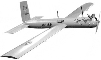
Controlled plant. A linear model of a real UAV called Silver Fox is developed, including the longitudinal and lateral dynamics, based on the aircraft parameters and the aerodynamic data. The Silver Fox is shown in Fig. 6. The fuselage of it is 1.8 meters long and the aircraft weighs 8.6 kilograms. The Silver Fox can carry small cameras and a Global Positioning System (GPS) receiver. It was originally developed by Advanced Ceramics Research (ACR).

Figure 6. The ‘Silver Fox’ UAV.
The linear model of the UAVs which consists of the longitudinal and lateral equations are respectively given by(Reference Choon26):
 $$\begin{eqnarray}
\left[\! \begin{array}{l@{\hspace*{4pt}}l}\Delta \dot{V} \\
\Delta \dot{\alpha } \\
\Delta \dot{q}\\
\Delta \dot{\theta }
\end{array} \right]&=& \left[ \begin{array}{c@{\hspace*{4pt}}c@{\hspace*{4pt}}c@{\hspace*{4pt}}c}-0.0785 & 6.0293 & -1.6485 & -9.7783 \\
-0.0489 & -3.9919 & -0.7386 & 0.0326\\
-0.0003 & -96.9781 & -260.2504 & 0\\
0 & 0 & 1 & 0 \end{array} \right] \left[ \begin{array}{l@{\hspace*{4pt}}l}\Delta V \\
\Delta \alpha \\
\Delta q\\
\Delta \theta \end{array} \right]\nonumber\\
&&+\, \left[ \begin{array}{c@{\hspace*{4pt}}c}-2.1657 & 1.4976 \\
-0.575 & -0.0052\\
-95.5596 & 0\\
0 & 0 \end{array} \right] \! \left[ \begin{array}{l@{\hspace*{4pt}}l}\Delta \delta _e \\
\Delta \delta _T \end{array} \right]
\end{eqnarray}$$
$$\begin{eqnarray}
\left[\! \begin{array}{l@{\hspace*{4pt}}l}\Delta \dot{V} \\
\Delta \dot{\alpha } \\
\Delta \dot{q}\\
\Delta \dot{\theta }
\end{array} \right]&=& \left[ \begin{array}{c@{\hspace*{4pt}}c@{\hspace*{4pt}}c@{\hspace*{4pt}}c}-0.0785 & 6.0293 & -1.6485 & -9.7783 \\
-0.0489 & -3.9919 & -0.7386 & 0.0326\\
-0.0003 & -96.9781 & -260.2504 & 0\\
0 & 0 & 1 & 0 \end{array} \right] \left[ \begin{array}{l@{\hspace*{4pt}}l}\Delta V \\
\Delta \alpha \\
\Delta q\\
\Delta \theta \end{array} \right]\nonumber\\
&&+\, \left[ \begin{array}{c@{\hspace*{4pt}}c}-2.1657 & 1.4976 \\
-0.575 & -0.0052\\
-95.5596 & 0\\
0 & 0 \end{array} \right] \! \left[ \begin{array}{l@{\hspace*{4pt}}l}\Delta \delta _e \\
\Delta \delta _T \end{array} \right]
\end{eqnarray}$$
 $$\begin{equation}
{\left[ \begin{array}{l@{\hspace*{4pt}}l}\Delta \dot{\beta } \\
\Delta \dot{p} \\
\Delta \dot{r}
\end{array} \right]\!=\! \left[ \begin{array}{c@{\hspace*{4pt}}c@{\hspace*{4pt}}c}-0.1798 & 0.069 & -0.9976 \\
-22.4565 & -8.213 & 2.0046 \\
15.0747 & -0.6578 & -0.7095 \end{array} \right] \left[ \begin{array}{l@{\hspace*{4pt}}l}\Delta \beta \\
\Delta p \\
\Delta r
\end{array} \right]\!+\! \left[ \begin{array}{c@{\hspace*{4pt}}c}0.0000 & 0.0873 \\
99.5144 & 2.4034\\
-7.9397 & -10.1124 \end{array} \right] \left[ \begin{array}{l@{\hspace*{4pt}}l}\Delta \delta _a \\
\Delta \delta _r \end{array} \right]}
\end{equation}$$
$$\begin{equation}
{\left[ \begin{array}{l@{\hspace*{4pt}}l}\Delta \dot{\beta } \\
\Delta \dot{p} \\
\Delta \dot{r}
\end{array} \right]\!=\! \left[ \begin{array}{c@{\hspace*{4pt}}c@{\hspace*{4pt}}c}-0.1798 & 0.069 & -0.9976 \\
-22.4565 & -8.213 & 2.0046 \\
15.0747 & -0.6578 & -0.7095 \end{array} \right] \left[ \begin{array}{l@{\hspace*{4pt}}l}\Delta \beta \\
\Delta p \\
\Delta r
\end{array} \right]\!+\! \left[ \begin{array}{c@{\hspace*{4pt}}c}0.0000 & 0.0873 \\
99.5144 & 2.4034\\
-7.9397 & -10.1124 \end{array} \right] \left[ \begin{array}{l@{\hspace*{4pt}}l}\Delta \delta _a \\
\Delta \delta _r \end{array} \right]}
\end{equation}$$
In the leader-following UAVs system, the dynamic models of the lead UAV and the wing UAVs in the simulation are the same.
Control problem and control objective. For the distributed leader-follower UAVs formation flight control problem with uncertain parameters given by Equations (6) and (7), we use the multivariable MRAC method to fulfill the state tracking of the wing UAVs. The objective of the UAVs formation flight control based on multivariable MRAC is to design bounded state feedback control laws ui (t) to make all the followers’ states xi (t) bounded and track the leader’s state x 0(t) asymptotically, i.e. lim t → ∞(xi (t) − x 0(t)) = 0.
Matching condition. For the distributed leader-following system with uncertain parameters, some matching conditions should be satisfied. The models of the lead UAV and the wing UAVs are the same, thus A 0 = Ai , B 0 = Bi (i = 1, 2, 3). However, the initial states of the lead UAV and the wing UAVs may be different. Ae is chosen to be the nominal closed-loop system matrix using the LQ method. Be = Bi (i = 1, 2, 3). Therefore, Assumption 3 and Assumption 4 are satisfied. In the UAVs formation flight control system, Assumption 5 is satisfied. In particular, Si can be any positive definite diagonal matrix(Reference Sang21,Reference Eugene, Ross and Irene27-Reference Sang and Tao31) .
Control method. To verify the effectiveness of the proposed multivariable MRAC method on system performance improvement, three control methods are adopted. The first is the fixed control which exactly is the nominal control described by Equation (11). The second is an existing adaptive control which is shown in Ref. 22. The last is a comparison proposed adaptive control described by Equation (14) with parameter adaptive laws. Here, we use MATLAB R2014a to simulate the above leader-following system. The adaptive control-based distributed formation flight control system is divided into the longitudinal and lateral controllers designed as follows.
Adaptive state feedback controller. According to the adaptive controller, Equation (14), with adaptive laws, Equation (15)–(17), the adaptive longitudinal and lateral controllers of the wing UAVs for the distributed leader-follower UAVs formation flight control problem with uncertain parameters are respectively designed by
 $$\begin{equation}
\Delta u_{lon_i}(t)=k_{1i,lon}^T(t)(\Delta x_{lon_i}(t)-\Delta x_{lon_0}(t))+k_{2ij,lon}(t)\Delta u_{lon_0}(t)+k_{3ij,lon}^T(t)\Delta x_{lon_0}(t)
\end{equation}$$
$$\begin{equation}
\Delta u_{lon_i}(t)=k_{1i,lon}^T(t)(\Delta x_{lon_i}(t)-\Delta x_{lon_0}(t))+k_{2ij,lon}(t)\Delta u_{lon_0}(t)+k_{3ij,lon}^T(t)\Delta x_{lon_0}(t)
\end{equation}$$
 $$\begin{equation}
\Delta u_{lat_i}(t)=k_{1i,lat}^T(t)(\Delta x_{lat_i}(t)-\Delta x_{lat_0}(t))+k_{2ij,lat}(t)\Delta u_{lat_0}(t)+k_{3ij,lat}^T(t)\Delta x_{lat_0}(t),
\end{equation}$$
$$\begin{equation}
\Delta u_{lat_i}(t)=k_{1i,lat}^T(t)(\Delta x_{lat_i}(t)-\Delta x_{lat_0}(t))+k_{2ij,lat}(t)\Delta u_{lat_0}(t)+k_{3ij,lat}^T(t)\Delta x_{lat_0}(t),
\end{equation}$$
where k 1i, lon , k 2ij, lon , k 3ij, lon , k 1i, lat , k 2ij, lat , k 3ij, lat are updated by Equations (15)–(17).
There is one lead UAV and three wing UAVs in the formation flight control system. The information interaction graph of them is presented in Fig. 7. For the longitudinal control, the initial leader and follower states are x 0 = [5 0 0 5/57.3] T , x 1 = [3 0 0 1/57.3] T , x 2 = [3 0 0 0] T and x 3 = [4 0 0 0] T , respectively. For the lateral control, the initial leader and followers states are x 0 = [5/57.3 0 0] T , x 1 = [4/57.3 0 0] T , x 2 = [2/57.3 0 0] T and x 3 = [3/57.3 0 0] T , respectively.
Figure 7. Interactions among one leader and three followers.
Based on the matching conditions, the nominal control gains can be calculated. They are used to show how a fixed controller cannot handle the parameter unknown case. The fixed controller is in the form of Equation (11) with controller parameters K*1ij, lon , K*2ij, lon , K*3ij, lon and K*1ij, lat , K*2ij, lat , K*3ij, lat being 80% and 60% of their nominal values, respectively. The form of the existing adaptive controller is shown with detail in Ref. 22, based on the unknown parameters for the followers. The comparison proposed adaptive controller is in the form of Equation (14) with parameter adaptive laws, Equation (15)–(17).
4.2 Simulation results and discussion
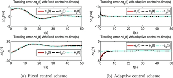
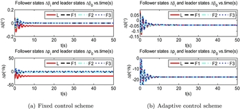
Simulation results. For the distributed leader-follower UAVs formation flight control problem with uncertain parameters, Figs 8 and 9 show the response results of the longitudinal state Δxlon = [ΔV, Δα, Δq, Δθ] T under the proposed adaptive control and fixed control. While Figs 14 and 15 show the response results of the lateral state Δxlat = [Δβ, Δp, Δr] T under the proposed adaptive control and fixed control. Figure 20 shows the control surfaces deflections of elevator, throttle, aileron and rudder under the proposed adaptive control and fixed control. Figures 10 and 11 and Figs 16 and 17 show the tracking error e(t) when the fixed control and the comparison proposed adaptive control, respectively, are applied to the Silver Fox on the same conditions. In addition, Figs 12 and 13 and Figs 18 and 19 show the tracking error e(t) when the existing adaptive control and the comparison proposed adaptive control, respectively, are applied to the Silver Fox on same conditions. Table 1 gives the final values of tracking errors comparison of the fixed control method, the existing MRAC method with the proposed multivariable MRAC method.

Figure 8. Follower states ΔVi and Δα i vs leader states with proposed MRAC vs fixed control.
Table 1 Tracking errors comparison

Performance analysis of the proposed adaptive control. Viewing from the proposed multivariable MRAC scheme in Figs 10 and 11 and Figs 16 and 17, all the flight states are bounded. A convergence of almost all state tracking errors to zero is observed, according to Table 1. While the final values of tracking errors of ΔV and Δα are within 1% of their steady values. It means that the flight states Δx loni = [ΔV, Δα, Δq, Δθ] T and Δx lati = [Δβ, Δp, Δr] T of the wing UAVs almost asymptotically track the states of the lead UAV when using the proposed multivariable MRAC scheme. When there exist parameter uncertainties for both the lead UAV and the wing UAVs, the closed-loop system has obtained the desired properties. The wing UAVs can still track the flight states of the lead UAV successfully.
Comparison of the proposed adaptive control and fixed control. Viewing from Figs 8(a) and 9(a) and Figs 14(a) and 15(a), the fixed control method cannot provide acceptable tracking performance since the followers fail to track the leader asymptotically. While in Figs 8(b) and 9(b) and Figs 14(b) and 15(b), we can clearly see the significant value the proposed MRAC scheme has to offer. According to the tracking errors in Figs 10 and 11 and Figs 16 and 17, we can see that the proposed multivariable MRAC scheme provides substantially improved performance over the fixed control method under the same flight conditions. As shown in Table 1, the final values of tracking errors for the fixed control fail to decay to zero, which leads to unacceptable tracking performance. It implies that the fixed controller cannot handle the parameter unknown case. The reason is that the fixed controller is obtained based on the known parameters, which is not accurate enough under parameter uncertainties. While the adaptive controller is based on the UAVs model with unknown parameters, whose parameters can be updated online through the adaptive control law. The simulation results demonstrate the effectiveness of the proposed multivariable MRAC method applied to the real flight control system. Therefore, the adaptive control will be more suitable for the real applications.

Figure 9. Follower states Δqi and Δθ i vs leader states with proposed MRAC vs fixed control.

Figure 10. Tracking errors ΔVe and Δα e with proposed MRAC vs fixed control.

Figure 11. Tracking errors Δqe and Δθ e with proposed MRAC vs fixed control.
Comparison of the proposed adaptive control and the existing adaptive control. Viewing from the tracking errors in Figs 12 and 13 and Figs 18 and 19, we can see that the tracking performance of the existing MRAC method is worse than that of the proposed multivariable MRAC scheme, as for the rapidity and the stability of the tracking error responses. As shown in Table 1, the final values of tracking errors for the existing adaptive control fail to converge to zero, which will result in greater errors with the increasement in flight time. The existing MRAC method can solve the problem with parametric uncertainties for the followers in the condition of a known reference model. However, when the reference is unknown, the existing MRAC method fails to guarantee that the system has good stability and tracking performance. On the contrary, the proposed multivariable MRAC method achieves good tracking performance even under parametric uncertainties for both the leader and the followers. Therefore, the proposed multivariable MRAC method is more suitable for solving the problem considering unknown model parameters for each UAV in the formation flight control system.

Figure 12. Tracking errors ΔVe and Δα e with proposed MRAC vs existing MRAC.

Figure 13. Tracking errors Δqe and Δθ e with proposed MRAC vs existing MRAC.

Figure 14. Follower states Δβ i and Δpi vs leader states with proposed MRAC vs fixed control.

Figure 15. Follower states Δri vs leader states with proposed MRAC vs fixed control.

Figure 16. Tracking errors Δβ e and Δpe with proposed MRAC vs fixed control.

Figure 17. Tracking errors Δre with proposed MRAC vs fixed control.

Figure 18. Tracking errors Δβ e and Δpe with proposed MRAC vs existing MRAC.

Figure 19. Tracking errors Δre with proposed MRAC vs existing MRAC.

Figure 20. Follower input vs leader input with proposed MRAC vs fixed control.
5.0 CONCLUSION
Formation flight is important for UAVs in improving the attack, reconnaissance and survival ability. In order to address the distributed leader-follower formation flight control problem of the multiple UAVs, a multivariable MRAC method is developed to solve the distributed leader-follower UAVs formation flight control problem. Unlike the existing MRAC method and the fixed control method, this proposed multivariable MRAC method is focused on the problem with uncertain parameters for both the leader and the followers. The adaption of the multivariable MRAC method enables UAVs to have good stability and tracking performance.
Simulation results demonstrate that the stability and tracking properties of the formation flight control system can be better achieved by the adaption of the proposed multivariable MRAC scheme, on control of the UAV called Silver Fox, compared with the fixed control method and the existing MRAC method.
For the adaptive state feedback state tracking control problem, the matching conditions in Section 3 are not easily satisfied in the UAVs formation flight control design. Therefore, it is important to relax the matching conditions to achieve the control objectives. This work presents the velocity and attitudes formation control for multiple UAVs formation. The trajectory tracking control for multiple UAVs formation needs to be addressed in future study.
ACKNOWLEDGEMENTS
This work was supported by the the National Natural Science Foundation of China (grant 61304223, 61673209, 61533008), the Fundamental Research Funds for the Central Universities (grant NJ20160026), the Aeronautical Science Foundation (grant 2016ZA52009), and the Foundation of Graduate Innovation Center in NUAA (grant kfjj20160326).