


NOMENCLATURE
 $ r_{MiT}(m)$
the range between missile and target
- $ r_{MiDi}(m)$
the range between missile and defender
- $ \textit{v}_{Mi}, \textit{v}_{Di},\ {\rm and}\ \textit{v}_{T}({\rm m/s})$
the speed of missile, defender, and target
- $ \gamma_{Mi}, \gamma_{Di},\ {and}\ \gamma_{T}({\rm rad})$
the flight-path angle of missile, defender, and target
- $ \lambda_{MiT}({\rm rad})$
the line-of-sight between missile and target
- $ \lambda_{MiDi}({\rm rad})$
the line-of-sight(LOS) between missile and defender
- $ a_{Mi}, a_{Di},\ {\rm and}\ a_{T}(m/s^{2})$
the acceleration of missile, defender, and target
- $ \tau_{Mi}, \tau_{Di},\ {\rm and}\ \tau_{T}(s)$
the time constant of missile, defender, and target
- $ y_{MiT}(m)$
the lateral displacements between missile and target
- $ y_{MiDi}(m)$
the lateral displacements between missile and defender
- $ \sigma_{i,\lambda}, \sigma_{i,y}({\rm mrad})$
the LOS angle and the lateral displacements measurement noise
- $ R_{k}(m)$
the lethality radius (LR) of the warhead
- $ M(m)$
the miss distance
- $ N_{j}^{i}$
the navigation gains
- $ Z_{j}^{i}$
the zero-effort-miss (ZEM) distance
- $ {\alpha_{i},\ \beta_{i},\ {\rm and}\ \eta}$
the weight coefficients


1.0 INTRODUCTION
In recent years, the problem of a target taking effective measures to respond to an incoming missile via proportional navigation (PN)(Reference Zarchan1), augmented proportional navigation (APN)(Reference Garber2), or optimal guidance laws (OGLs)(Reference Cottrell3) has received widespread attention. One of the solutions is the use of a defender to intercept the attacking missile before it intercepts the target. This is called as a target–missile–defender (TMD) scenario(Reference Boyell4–Reference Mitchell and Dimitra7) and also as three-body guidance.
The TMD problem was first proposed and studied by Boyell(Reference Boyell4,Reference Boyell5) , who assumed that the rate of speed change is constant and that both the interceptor and the defender use PN guidance. Accordingly, closed-form solutions of three-aircraft movements were obtained and analysed. With the development of combat styles and the continuous improvement in missile weapon performance, such problems have significantly attracted attention in recent years. Ratnoo and Shima(Reference Ratnoo and Shima8) geometrically analysed the relative motions of a target, missile, and defender and conducted simulation studies on different initial scenarios and guidance laws. Yamasaki and Balakrishnan(Reference Yamasaki and Balakrishnan9) provided a line-of-sight (LOS) guidance method for a defender. This method ensures that the trajectory of the defender is straight and that the defence success rate is high. In the simulation, a scenario of three aircrafts moving in a three-dimensional space was considered. In the above research, the target and the defender completed their respective tasks without cooperating with each other. To improve the viability of a target, a guidance law that permits the target and the defender to cooperate with each other was designed. Shaferman and Shima(Reference Shaferman and Shima10) proposed a multiple model adaptive guidance strategy for the TMD problem. This strategy is advantageous when considering detection errors and non-linear motion models and can design the cooperative guidance law between the target and the defender simultaneously.
Based on the engineering applications and research results of traditional guidance methods, LOS-based guidance methods have received attention for TMD problems. Balakrishnanetal.(Reference Yamasaki, Balakrishnan and Takano11) and Shima et al.(Reference Ratnoo and Shima12) published research results based on LOS guidance methods. Balakrishnan et al.(Reference Yamasaki, Balakrishnan and Takano11) improved the guidance law and studied different manoeuvre scenarios of a target. Shima et al.(Reference Ratnoo and Shima12) studied different interceptor guidance laws for defence strategies. In addition, Shima et al.(Reference Ratnoo and Shima13) studied an LOS-based guidance method for a defender and compared the proposed method with PN. The results showed that the LOS-based guidance method required a smaller overload to achieve combat objectives than the interceptor. With advancements in research, scholars have considered more practical and complex combat three-aircraft scenarios. In the case all the three systems can provide their current relative motion information in real time, the methods by which all the three bodies adopt the best manoeuvring strategy so that the final result is the most advantageous were studied. Shima(Reference Shima14) proposed an optimal cooperative guidance law based on the different linear guidance laws adopted by an interceptor to derive the respective optimal cooperative guidance laws for a target–defender team. A cost function that comprehensively considered energy consumption and miss distance(Reference Guo, Wang, Yao and Yang15) was proposed by Rubinsky et al.(Reference Rubinsky and Gutman16), who studied the strategies of a high-value aircraft and a defender based on the concept of optimal control. Moreover, they analysed the influence of different initial relative positions and the guidance remaining time on the interception results. Shima et al.(Reference Ratnoo and Shima17) also analysed the influence of the PN, pure pursuit, and LOS guidance adopted by a defender and an interceptor on the final guidance results and provided the conditions for them to achieve the combat objective.
To improve cooperation between a target and a defender, Shima et al.(Reference Prokopov and Shima18) proposed two-way cooperative strategies based on optimal control and provided the optimal two-way cooperative guidance law among the different ones adopted by an interceptor. Compared with one-way cooperative strategies, two-way cooperative strategies have clear advantages in terms of the miss distance and the control effort because the target and the defender can share information with each other regarding their future manoeuvres. Actually, in this case, the target plays a luring role so that the defender can intercept the interceptor well. Weiss et al.(Reference Weiss19) proposed the minimum effort guidance law for a defender to an interceptor and for a target to an evader from the interceptor. This guidance algorithm design for the TMD problem was based on the specification of the desired performance in terms of the miss distance and on optimisation of the effort required to achieve it. Based on the study by Shaferman and Shima(Reference Shaferman and Shima20), Fonod and Shima(Reference Fonod and Shima21) conceived the TMD problem as a scenario in which an aircraft launches two defenders to intercept an enemy interceptor. By introducing the error model of cooperative measurement, the effect of the relative measurement baseline between the two defenders on the detection and interception performance of the interceptor was studied. Moreover, the range of the best relative measurement angle that can improve the detection performance was determined.
Considering that both the missile and the target–defender team adopt a zero-sum game confrontation guidance form to achieve best respective guidance results, the differential game theory(Reference Perelman, Shima and Rusnak22–Reference Shalumov24) has been used to design their guidance laws. Using a linear-quadratic differential game formulation to establish a cost function, Perelman and Shima(Reference Perelman, Shima and Rusnak22) considered the miss distance and control effort of a missile and a target-defender team and provided analytical solutions for the control inputs of the three components. The conditions for the existence of a saddle-point solution were derived, and the navigation gains were analysed for various limiting cases. Rubinsky and Gutman(Reference Rubinsky and Gutman23) studied the differential game guidance law with a boundary control of the three components and presented algebraic conditions for a pursuer to capture an evader while evading a defender. In addition, the study provided the switch time at which the missile stops evading the defender and starts pursuing the target, and it was found that the switch occurs before the missile passes the defender. Shalumov(Reference Shalumov24) studied a more complex TMD engagement scenario in which a target faces the interception of two missiles and launches two defenders to counter-intercept to achieve penetration. By assuming the unknown guidance law of missiles, the confrontation between the target-defenders team and the missiles was treated as a zero-sum game problem, and their analytical solution was provided by a differential game.
This paper proposes a two-way cooperative guidance law based on the optimal control(Reference Mouada, Pavic and Pavkovic25) of a target and two defenders when the target faces two enemy missiles and launches two defenders to achieve anti-interception to protect the target. The two-way cooperative strategies ensure the target and the defenders fully cooperate with each other, allowing the defenders to intercept the missiles successfully by less control effort. To realise the identified guidance laws of the missiles and estimate their states, a multiple-mode adaptive estimator (MMAE) is introduced. Each model in the MMAE represents a possible guidance law or guidance parameters adopted by the missiles, and the target and the defenders can select different guidance strategies for different missile guidance laws identified by the MMAE.
The remainder of this paper is organised as follows. In Section1, the cooperative interception engagement model is described, and the measurement model and the cost function are introduced. In Section2, the two-way cooperative optimal guidance law is presented, which considers the control of the target and the two defenders in the same cost function so that they can fully cooperate with each other. In Section3, the MMAE is introduced to identify the guidance laws adopted by the missiles and estimate their states. A combined MMAE and two-way cooperative optimal guidance law is implemented in simulations, and the verification of the results is presented in Section4. The main findings of this study are summarised in Section5.
2.0 PROBLEM STATEMENT
When a high-value aircraft (target) is engaged by two enemy homing missiles, two defenders need to be launched by the target to intercept the missiles for protecting itself. The engagement scenario includes a target, two defenders, and two missiles, which adopt the existing guidance laws to intercept the target.
Dynamic and kinematic models are established in the inertial coordinate system.  ${X_I} - {O_I} - {Y_I}$, as shown in Fig. 1, is the planar engagement geometry of the target, two missiles, and two defenders. We denote the variables associated with the target, two missiles, and two defenders as
  $T$,
$T$,  $Mi$, and
  $Di$, respectively. The normal acceleration, speed, LOS, range, and flight-path angle are denoted as
  $a$,
$a$,  $v$,
$v$,  $\lambda $,
  $r$, and
  $\gamma $, respectively.
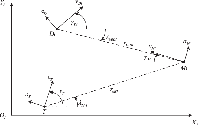
Figure 1. Planar engagement geometry.
2.1 Kinematics and dynamics
Neglecting the influence of gravity, the engagement process between the target and the missiles can be expressed in the form of polar coordinates  $(r,\lambda )$ as follows:
 \begin{equation}{\dot r_{MiT}} = {v_{MiT}} = - {v_T}\cos ({\gamma _T} - {\lambda _{MiT}}) - {v_{Mi}}\cos ({\gamma _{Mi}} + {\lambda _{MiT}}); i = \{ 1,2\} \end{equation}
 \begin{equation}{\dot \lambda _{MiT}} = \frac{{{v_T}\sin ({\gamma _T} - {\lambda _{MiT}}) - {v_{Mi}}\sin ({\gamma _{Mi}} + {\lambda _{MiT}})}}{{{r_{MiT}}}};i = \{ 1,2\}\end{equation}
Similarly, the engagement kinematic equations between the defenders and the missiles can be expressed as
 \begin{equation}{\dot r_{MiDi}} = {v_{MiDi}} = - {v_{Di}}\cos ({\gamma _{Di}} - {\lambda _{MiDi}}) - {v_{Mi}}\cos ({\gamma _{Mi}} + {\lambda _{MiDi}}); i = \{ 1,2\} \end{equation}
 \begin{equation}{\dot \lambda _{MiDi}} = \frac{{{v_{Di}}\sin ({\gamma _{Di}} - {\lambda _{MiDi}}) - {v_{Mi}}\sin ({\gamma _{Mi}} + {\lambda _{MiDi}})}}{{{r_{MiDi}}}}; i = \{ 1,2\}\end{equation}
Above,  ${\dot r_{MiT}}$ and
  ${\dot \lambda _{MiT}}$ are the relative velocity and the LOS velocity between the missiles and the target, respectively, and
  ${\dot r_{MiDi}}$ and
  ${\dot \lambda _{MiDi}}$ are those between the missiles and the defenders, respectively.
The normal acceleration of the aircraft, perpendicular to its motion (velocity), is denoted as  $a$. During the entire guidance process, the speeds of the target, defenders, and missiles are maintained constant. The relationship between the normal acceleration and flight-path angle of each aircraft can be obtained as
 \begin{equation}{\dot \gamma _i} = \frac{{{a_i}}}{{{v_i}}}; i = \{ T,M1,M2,D1,D2\} \end{equation}
During the engagement, it is assumed that the aircraft dynamics can be represented by arbitrary-order linear equations as follows:
 \begin{equation}\left\{ \begin{array}{c@{\quad}c@{\quad}c@{\quad}c}{{{{\dot{\textbf{\textit{x}}}}}_i} = {{\textbf{\textit{A}}}_i}{{\textbf{\textit{x}}}_i} + {{\textbf{\textit{B}}}_i}{u_i}}\\[5pt]{{a_i} = {{\textbf{\textit{C}}}_i}{{\textbf{\textit{x}}}_i} + {d_i}{u_i}}\end{array} \right.\!\!\!\!\!,{\kern 1pt} {\kern 1pt} {\kern 1pt} {\kern 1pt} {\kern 1pt} {\kern 1pt} i = \{ T,M1,M2,D1,D2\}\end{equation}
where  ${{\textbf{\textit{x}}}_i}$ is an aircraft individual state vector and
  ${u_i}$ is the corresponding control input. When first-order linear dynamics with the time constant
  ${\tau _i}$ is considered for the aircraft, parameters
  ${{\textbf{\textit{A}}}_i} = {{ - 1}/{{\tau _i}}} $,
  ${{\textbf{\textit{B}}}_i} = 1/ {{\tau _i}}$,
  ${{\textbf{\textit{C}}}_i} = 1$, and
  ${d_i} = 0$ can be adopted.
Remark 1. When the flight process of two aircrafts is approximately a nominal collision triangle, the process can be linearised. In the engagement scenario depicted in Fig. 1, two collision triangles are formed between the target and the missiles, and between the defenders and the missiles, respectively.
After linearisation, the state vector can be selected as
 \begin{align}{\textbf{\textit{x}}} = {\left[ \begin{array}{c@{\quad}c@{\quad}c@{\quad}c@{\quad}c@{\quad}c@{\quad}c@{\quad}c@{\quad}c}{{{\textbf{\textit{x}}}_{M1T}}} &{{{\textbf{\textit{x}}}_{M2T}}} &{{{\textbf{\textit{x}}}_{M1D1}}} & {{{\textbf{\textit{x}}}_{M2D2}}} & {{{\textbf{\textit{x}}}_{M1}}} & {{{\textbf{\textit{x}}}_{M2}}} & {{{\textbf{\textit{x}}}_{D1}}} & {{{\textbf{\textit{x}}}_{D2}}} & {{{\textbf{\textit{x}}}_T}}\end{array} \right]^T}\nonumber\\[-18pt]\end{align}
where  ${{\textbf{\textit{x}}}_{MiT}} = {\left[ \begin{array}{c@{\quad}c}{{y_{MiT}}} & {{{\dot y}_{MiT}}}\end{array} \right]^T}$,
  ${{\textbf{\textit{x}}}_{MiDi}} = {\left[ \begin{array}{c@{\quad}c}{{y_{MiDi}}} & {{{\dot y}_{MiDi}}}\end{array} \right]^T}$, and
  $i = \{ 1,2\} $;
  ${y_{MiT}}$ and
  ${y_{MiDi}}$ are the lateral displacements between the target and the missiles and between the defenders and the missiles, respectively; and
  ${\dot y_{MiT}}$ and
  ${\dot y_{MiDi}}$ are the corresponding lateral relative velocities between them.
The state equation of the relative motion of the aircraft can be written as
 \begin{align}{\dot{\textbf{\textit{x}}}} = \left\{ \begin{array}{l}{{\dot x}_1} = {x_2}\\[2pt]{{\dot x}_2} = {a_T} - {a_{M1}}\\[2pt]{{\dot x}_3} = {x_4}\\[2pt]{{\dot x}_4} = {a_T} - {a_{M2}}\\[2pt]{{\dot x}_5} = {x_6}\\[2pt]{{\dot x}_6} = {a_{M1}} - {a_{D1}}\\[2pt]{{\dot x}_7} = {x_8}\\[2pt]{{\dot x}_8} = {a_{M2}} - {a_{D2}}\\[2pt]{{{\dot{\textbf{\textit{x}}}}}_{M1}} = {{\textbf{\textit{A}}}_{M1}}{{\textbf{\textit{x}}}_{M1}} + {{\textbf{\textit{B}}}_{M1}}{u_{M1}}\\[2pt]{{{\dot{\textbf{\textit{x}}}}}_{M2}} = {{\textbf{\textit{A}}}_{M2}}{{\textbf{\textit{x}}}_{M2}} + {{\textbf{\textit{B}}}_{M2}}{u_{M2}}\\[2pt]{{{\dot{\textbf{\textit{x}}}}}_{D1}} = {{\textbf{\textit{A}}}_{D1}}{{\textbf{\textit{x}}}_{D1}} + {{\textbf{\textit{B}}}_{D1}}{u_{D1}}\\[2pt]{{{\dot{\textbf{\textit{x}}}}}_{D2}} = {{\textbf{\textit{A}}}_{D2}}{{\textbf{\textit{x}}}_{D2}} + {{\textbf{\textit{B}}}_{D2}}{u_{D2}}\\[2pt]{{{\dot{\textbf{\textit{x}}}}}_T} = {{\textbf{\textit{A}}}_T}{{\textbf{\textit{x}}}_T} + {{\textbf{\textit{B}}}_T}{u_T}\end{array} \right.\end{align}
Equation (8) can be represented by the state-space equation as follows:
 \begin{align}{\dot{\textbf{\textit{x}}}} = {\textbf{\textit{Ax}}}(t) + {\textbf{\textit{B}}}\left[ \begin{array}{c@{\quad}c@{\quad}c}{{u_T}} & {{u_{D1}}} & {{u_{D2}}}\end{array} \right]^T + {\textbf{\textit{C}}}\left[ \begin{array}{c@{\quad}c}{{u_{M1}}} & {{u_{M2}}}\end{array} \right]^T + w(t)\nonumber\\[-18pt]\end{align}
where
 \begin{equation*}{\textbf{\textit{A}}} = \left[ \begin{array}{c@{\quad}c@{\quad}c}{{{\textbf{\textit{A}}}_{11}}} & {\left[ 0 \right]} & {{{\textbf{\textit{A}}}_{13}}}\\[3pt]{\left[ 0 \right]} & {{{\textbf{\textit{A}}}_{22}}} & {{{\textbf{\textit{A}}}_{23}}}\\[3pt]{\left[ 0 \right]} & {\left[ 0 \right]} & {{{\textbf{\textit{A}}}_{33}}}\end{array} \right]\\[3pt]{\textbf{\textit{B}}} = \left[ \begin{array}{c@{\quad}c@{\quad}c}{{{\textbf{\textit{B}}}_{11}}} & {\left[ 0 \right]} & {\left[ 0 \right]}\\[3pt]{\left[ 0 \right]} & {{{\textbf{\textit{B}}}_{22}}} & {{{\textbf{\textit{B}}}_{23}}}\\[3pt]{{{\textbf{\textit{B}}}_{31}}} & {{{\textbf{\textit{B}}}_{32}}} & {{{\textbf{\textit{B}}}_{33}}}\end{array} \right]\\[3pt]{\textbf{\textit{C}}} = \left[ \begin{array}{c@{\quad}c}{{{\textbf{\textit{C}}}_{11}}} & {{{\textbf{\textit{C}}}_{12}}}\\[3pt]{{{\textbf{\textit{C}}}_{21}}} & {{{\textbf{\textit{C}}}_{22}}}\\[3pt]{{{\textbf{\textit{C}}}_{31}}} & {{{\textbf{\textit{C}}}_{32}}}\end{array} \right]\end{equation*}
and
 \begin{align*}{{\textbf{\textit{A}}}_{11}} & = \left[ \begin{array}{c@{\quad}c@{\quad}c@{\quad}c}0 & 1 & 0 & 0\\[3pt]0 & 0 & 0 & 0\\[3pt]0 & 0 & 0 & 1\\[3pt]0 & 0 & 0 & 0\end{array} \right],\!\!\quad {{\textbf{\textit{A}}}_{13}} = \left[ \begin{array}{c@{\quad}c@{\quad}c@{\quad}c@{\quad}c}0 & 0 & 0 & 0 & 0\\[3pt]{ - {{\textbf{\textit{C}}}_{M1}}} & 0 & 0 & 0 & {{{\textbf{\textit{C}}}_T}}\\[3pt]0 & 0 & 0 & 0 & 0\\[3pt]0 & { - {{\textbf{\textit{C}}}_{M2}}} & 0 & 0 & {{{\textbf{\textit{C}}}_T}}\end{array} \right],\!\!\quad {{\textbf{\textit{A}}}_{22}} = \left[ \begin{array}{c@{\quad}c@{\quad}c@{\quad}c}0 & 1 & 0 & 0\\[3pt]0 & 0 & 0 & 0\\[3pt]0 & 0 & 0 & 1\\[3pt]0 & 0 & 0 & 0\end{array} \right],\\[9pt]{{\textbf{\textit{A}}}_{23}} & = \left[ \begin{array}{c@{\quad}c@{\quad}c@{\quad}c@{\quad}c}0 & 0 & 0 & 0 & 0\\[3pt]{ - {{\textbf{\textit{C}}}_{M1}}} & 0 & {{{\textbf{\textit{C}}}_{D1}}} & 0 & 0\\[3pt]0 & 0 & 0 & 0 & 0\\[3pt]0 & { - {{\textbf{\textit{C}}}_{M2}}} & 0 & {{{\textbf{\textit{C}}}_{D2}}} & 0\end{array} \right]\end{align*}
 \begin{align*}{{\textbf{\textit{A}}}_{33}} & = \left[ \begin{array}{c@{\quad}c@{\quad}c@{\quad}c@{\quad}c}{{{\textbf{\textit{A}}}_{M1}}} & 0 & 0 & 0 & 0\\[3pt]0 & {{{\textbf{\textit{A}}}_{M2}}} & 0 & 0 & 0\\[3pt]0 & 0 & {{{\textbf{\textit{A}}}_{D1}}} & 0 & 0\\[3pt]0 & 0 & 0 & {{{\textbf{\textit{A}}}_{D2}}} & 0\\[3pt]0 & 0 & 0 & 0 & {{{\textbf{\textit{A}}}_T}}\end{array} \right]\quad {{\textbf{\textit{B}}}_{11}} = \left[ \begin{array}{c}0\\[3pt]{{d_T}}\\[3pt]0\\[3pt]{{d_T}}\end{array} \right]\quad {{\textbf{\textit{B}}}_{22}} = \left[ \begin{array}{c}0\\[3pt]{{d_{D1}}}\\[3pt]0\\[3pt]0\end{array} \right]\quad {{\textbf{\textit{B}}}_{23}} = \left[ \begin{array}{c}0\\[3pt]0\\[3pt]0\\[3pt]{{d_{D2}}}\end{array} \right]\\[9pt]{{\textbf{\textit{B}}}_{31}} & = \left[ \begin{array}{c}0\\[3pt]0\\[3pt]0\\[3pt]0\\[3pt]{{{\textbf{\textit{B}}}_T}}\end{array} \right]\quad{{\textbf{\textit{B}}}_{32}} = \left[ \begin{array}{c}0\\[3pt]0\\[3pt]{{{\textbf{\textit{B}}}_{D1}}}\\[3pt]0\\[3pt]0\end{array} \right] \quad {{\textbf{\textit{B}}}_{33}} = \left[ \begin{array}{c}0\\[3pt]0\\[3pt]0\\[3pt]{{{\textbf{\textit{B}}}_{D2}}}\\[3pt]0\end{array} \right]\quad {{\textbf{\textit{C}}}_{11}} = \left[ \begin{array}{c}0\\[3pt]{ - {d_{M1}}}\\[3pt]0\\[3pt]0\end{array} \right]\quad {{\textbf{\textit{C}}}_{12}} = \left[ \begin{array}{c}0\\[3pt]0\\[3pt]0\\[3pt]{ - {d_{M2}}}\end{array} \right]\\[8pt] {{\textbf{\textit{C}}}_{21}} & = \left[ \begin{array}{c}0\\[3pt]{ - {d_{M1}}}\\[3pt]0\\[3pt]0\end{array} \right]\quad {{\textbf{\textit{C}}}_{22}} = \left[ \begin{array}{c}0\\[3pt]0\\[3pt]0\\[3pt]{ - {d_{M2}}}\end{array} \right]\quad {{\textbf{\textit{C}}}_{31}} = \left[ \begin{array}{c}{{{\textbf{\textit{B}}}_{M1}}}\\[3pt]0\\[3pt]0\\[3pt]0\\[3pt]0\end{array} \right]\quad {{\textbf{\textit{C}}}_{32}} = \left[ \begin{array}{c}0\\[3pt]{{{\textbf{\textit{B}}}_{M2}}}\\[3pt]0\\[3pt]0\\[3pt]0\end{array} \right]\end{align*}
Control input  ${u_i}$, where
  ${\kern 1pt} i = \{ T,M1,M2,D1,D2\} $, satisfies the condition,
  $\left| {{u_i}} \right| \le u_i^{\max }$, and
  $w$ is the noise in the guidance process.
2.2 Timeline
The initial range between the target and the missiles are denoted as  ${r_{Mi{T_0}}}$. Similarly, that between the defender and missiles is
  ${r_{MiD{i_0}}}$. Under the assumption that in the nominal collision triangle, the deviation between the flightpath and LOS angles is small, the times of the missiles-to-target and defenders-to-missiles interceptions are determined as follows:
 \begin{align}t_f^{MiT} & = \frac{{ - {r_{Mi{T_0}}}}}{{{{\dot r}_{Mi{T_0}}}}}\nonumber\\[2pt]& = \frac{{{r_{Mi{T_0}}}}}{{{v_T}\cos \left({\gamma _{{T_0}}} - {\lambda _{Mi{T_0}}}\right) + {v_{Mi}}\cos \left({\gamma _{M{i_0}}} + {\lambda _{Mi{T_0}}}\right)}}; i = \{ 1,2\}\end{align}
 \begin{align}t_f^{MiDi} & = \frac{{ - {r_{MiD{i_0}}}}}{{{{\dot r}_{MiD{i_0}}}}}\nonumber\\[2pt]& = \frac{{{r_{MiD{i_0}}}}}{{{v_{Di}}\cos \left({\gamma _{D{i_0}}} - {\lambda _{MiD{i_0}}}\right) + {v_{Mi}}\cos \left({\gamma _{M{i_0}}} + {\lambda _{MiD{i_0}}}\right)}}; i = \{ 1,2\} \end{align}
Remark 2.  $\Delta {t_i} = {t_{fMiT}} - {t_{fMiDi}}$ is defined as the deviation between the missiles-to-target and defenders-to-missiles interceptions. To complete the combat task, the defenders should intercept the missiles maximally rapidly; therefore, the time deviation satisfies
  $\Delta {t_i} \gt 0$.
The missiles-to-target time-to-go,  $t_{go}^{MiT}$, and the defenders-to-missiles time-to-go,
  $t_{go}^{MiDi}$, can be defined as follows:
 \begin{equation*}t_{go}^{MiT} = t_f^{MiT} - t, t_{go}^{MiDi} = t_f^{MiDi} - t\end{equation*}
2.3 Measurement model
It is assumed that both the target and the defenders can measure the LOS angle,  ${\lambda _{MiT}}$, or
  ${\lambda _{MiDi}}$ using an infrared (IR) sensor. In addition, each sensor is contaminated by white Gaussian noises
  ${v_i}$, where
  $i = \{ M1T,M2T,M1D1,M2D2\} $, which are mutually independent during the measurement. We assume that the LOS angle measurement noise of each agent obeys the distribution,
 \begin{equation}v_i^\lambda \sim N\left(0,\sigma _{i,\lambda }^2\right); i = \{ M1T,M2T,M1D1,M2D2\} \end{equation}
Applying the small-angle approximation, the linearised measurement of the lateral separation can be obtained as
 \begin{align}{y_i} & = {r_i}\sin ({\lambda _i} + {\sigma _{i,\lambda }})\nonumber\\[3pt] &\approx {r_i}{\lambda _i} + {r_i}{\sigma _{i,\lambda }};\quad i = \{ M1T,M2T,M1D1,M2D2\} \end{align}
Because two-way cooperative strategies are adopted by the target-defenders team, the linearised measurement noise,  ${\sigma _{i,y}}$, and the measurement matrix,
  ${\textbf{\textit{H}}}$, can be expressed as
 \begin{equation}{\sigma _{i,y}} \buildrel \Delta \over = {r_i}{\sigma _{i,\lambda }} \sim N\left(0,{\left({r_i}{\sigma _{i,\lambda }}\right)^2}\right)\end{equation}
 \begin{equation}{\textbf{\textit{H}}} = \left[ \begin{array}{c@{\quad}c@{\quad}c@{\quad}c@{\quad}c@{\quad}c@{\quad}c@{\quad}c@{\quad}c@{\quad}c@{\quad}c@{\quad}c@{\quad}c}1 & 0 & 0 & 0 & 0 & 0 & 0 & 0 & 0 & 0 & 0 & 0 & 0\\[3pt]0 & 0 & 1 & 0 & 0 & 0 & 0 & 0 & 0 & 0 & 0 & 0 & 0\\[3pt]0 & 0 & 0 & 0 & 1 & 0 & 0 & 0 & 0 & 0 & 0 & 0 & 0\\[3pt]0 & 0 & 0 & 0 & 0 & 0 & 1 & 0 & 0 & 0 & 0 & 0 & 0\end{array}\right]\end{equation}
Moreover, the measurement equation can be expressed as follows:
 \begin{align} {\textbf{\textit{z}}} & = {\textbf{\textit{Hx}}} + {{\textbf{\textit{v}}}^y},{{\textbf{\textit{v}}}^y}\ \sim\ N\left({\left[ 0 \right]_{4 \times 1}},{\textbf{\textit{R}}}\right),\nonumber\\[4pt] {\textbf{\textit{R}}} & = diag\left\{ {\sigma _{M1T,y}},{\sigma _{M2T,y}},{\sigma _{M1D1,y}},{\sigma _{M2D2,y}}\right\} \end{align}
Assuming that the target does not cooperate with the defenders, the defenders cannot obtain the measurements from the target. The measurement matrix,  ${\textbf{\textit{H}}}$, and the measurement equation can be expressed as follows:
 \begin{equation}{\textbf{\textit{H}}} = \left[ \begin{array}{c@{\quad}c@{\quad}c@{\quad}c@{\quad}c@{\quad}c@{\quad}c@{\quad}c@{\quad}c@{\quad}c@{\quad}c@{\quad}c@{\quad}c}0 & 0 & 0 & 0 & 1 & 0 & 0 & 0 & 0 & 0 & 0 & 0 & 0\\[5pt]0 & 0 & 0 & 0 & 0 & 0 & 1 & 0 & 0 & 0 & 0 & 0 & 0\end{array} \right]\end{equation}
 \begin{align} {\textbf{\textit{z}}} & = {\textbf{\textit{Hx}}} + {{\textbf{\textit{v}}}^y},{{\textbf{\textit{v}}}^y} \sim N\left({\left[ 0 \right]_{2 \times 1}},{\textbf{\textit{R}}}\right),\nonumber\\[4pt]{\textbf{\textit{R}}} & = diag\left\{ {\sigma _{M1D1,y}},{\sigma _{M2D2,y}}\right\} \end{align}
2.4 Performance index
Successful interception of missiles requires a minimal miss distance or even a direct hit. However, owing to the influence of various factors, defenders cannot directly hit missiles with high accuracy. In particular, the state estimation method for missiles severely restricts the guidance accuracy. A realistic lethality model influenced by many factors is difficult to obtain; therefore, we propose a simplified lethality function to evaluate the probability of destroying a target, which is expressed as follows:
 \begin{align}{P_d}(M,{R_k}) = \left\{ \begin{array}{l@{\quad}l}1 & M \le {R_k}\\[3pt] 0 & M \gt {R_k}\end{array} \right.\end{align}
where  ${R_k}$ is the lethality radius (LR) of the warhead and
  $M$ is the miss distance between the defenders and the missiles. When the miss distance is shorter than the LR of the warhead, the interception is successful.
Remark 3. The index of successfully intercepting a target is the miss distance, which is influenced by the manoeuvre form and the detection noise, and is a random variable. Typically the cumulative distribution function (CDF) is used as an empirical estimate to evaluate the impact of miss distance on guidance accuracy. It is also employed to compare the performance of different guidance laws. Therefore, we can determine the success of an interception in advance based on the determined kill probability under the given LR condition.
This kill probability is defined as
 \begin{align}{SSKP}({R_k}) = E\left\{ {P_d}(M,{R_k})\right\}\nonumber\\[-18pt] \end{align}
where  $E$ is the mathematical expectation with respect to the miss distance random variable, and
  $\text{SSKP}({R_k})$ can be calculated by the CDF. It follows that
 \begin{align}{SSKP}({R_k}) &= \int_{ - \infty }^\infty {{P_d}(M,{R_k}){f_M}(m)} dm\nonumber\\[6pt] &= \int_0^{{R_k}} {{f_M}(m)dm = pr\left(M \le {R_k}\right) \buildrel \Delta \over = {F_M}\left({R_k}\right)} \end{align}
where  ${f_M}$ and
  ${F_M}$ are the probability density function (PDF) and the CDF, respectively. The probability of interception is frequently taken as 0.95, yielding the following performance index:
 \begin{align}J = \mathop {\arg }\limits_{{R_k}} \{ \text{SSKP}({R_k}) = 0.95\}\nonumber\\[-18pt] \end{align}
This performance index has to be minimised by the defenders.
3.0 DESIGN OF COOPERATIVE GUIDANCE
Here, we provide a more detailed description of the engagement problem proposed in Section2, where the target–defenders team uses two-way cooperative strategies to intercept the missiles. Compared with the one-way cooperative strategies that only take the cooperation between the defender into account, the two-way cooperative strategies ensure the target and the defenders fully cooperate with each other. Specifically, the target can act as a bait to perform lure manoeuvres so that the defenders can intercept the missiles accurately and effectively. Concurrently, the defenders can obtain the manoeuvring sequence of the target to predict the intercepting point with the missiles and head towards it. The main problems to be considered in the design of the guidance law are that the control inputs of the target and the defenders need to be included in the same cost function. Consequently, the missiles can be intercepted by minimising the control efforts of the target and the defenders.
3.1 Missile guidance law
Some of the commonly used missile guidance laws used in terminal guidance to intercept stationary and manoeuvring targets are PN, APN, and OGLs. Under perfect information and linear kinematics, these guidance laws can be written as follows(Reference Zarchan1):
 \begin{equation}{u_{Mi}} = N_j^i\dfrac{{Z_j^i}}{{{{\left(t_{go}^{MiT}\right)}^2}}}; \quad j = \{ {\rm{PN}},{\rm{APN}},{\rm{OGL}}\} \end{equation}
where  $N_j^i$ denotes the navigation gains of the missiles, which range from 3 to 5, and
  $Z_j^i$ is the zero-effort-miss (ZEM) distance. The ZEM represents the miss distance under the conditions that the target follows an assumed manoeuvring model and that no further acceleration commands are executed by the missiles from the current time and until the end of the engagement.
The navigation gains,  $N_j^i$ and
  $Z_j^i$, of PN, APN, and OGLs can be expressed as
 \begin{equation}N_{{\rm{PN}}}^i = 3 \sim 5;{\kern 1pt} {\kern 1pt} {\kern 1pt} {\kern 1pt} {\kern 1pt} {\kern 1pt} {\kern 1pt} {\kern 1pt} {\kern 1pt} {\kern 1pt} Z_{{\rm{PN}}}^i = {y_{MiT}} + {\dot y_{MiT}}t_{go}^{MiT}\end{equation}
 \begin{equation}N_{{\rm APN}}^{i} =3 \sim 5;{\kern 1pt} {\kern 1pt} {\kern 1pt} {\kern 1pt} {\kern 1pt} {\kern 1pt} {\kern 1pt} {\kern 1pt} {\kern 1pt} {\kern 1pt} Z_{{\rm APN}}^{i} ={\kern 1pt} Z_{{\rm APN}}^{i} +{a_{T} \left(t_{go}^{MiT} \right)^{2}/2}\end{equation}
 \begin{equation}{\kern 1pt} Z_{{\rm OGL}}^{i} ={\kern 1pt} Z_{{\rm APN}}^{i} -a_{Mi} \tau _{Mi}^{2} \psi \left({t_{go}^{MiT}/\tau_{Mi} } \right)\end{equation}
where  ${\tau _{Mi}}$ is the dynamics time constant of a missile, and
  $\psi (\xi ) = \exp ( - \xi ) + \xi - 1$.
 \begin{equation}N_{{\rm OGL}}^{i} =\frac{6\theta _{MiT}^{2} \psi (\theta _{MiT} )}{3+6\theta _{MiT} -6\theta _{MiT}^{2} +2\theta _{MiT}^{3} -3e^{-2\theta _{MiT} } -12\theta _{MiT} e^{-\theta _{MiT} } +6{a_{i}/\tau _{Mi}^{3} } }\end{equation}
where  ${\theta _{MiT}} = {t_{go}^{MiT}}/{{\tau _{Mi}}} $ is the normalised time-to-go and
  ${a_i}$ represents the weight ratio of the miss distance and the control effort in the cost function,
 \begin{equation}J_{Mi} =\frac{\alpha _{i} }{2} ({\rm miss})^{2} +\frac{1}{2} \int _{0}^{t_{f}^{MiDi} }u_{Mi}^{2} dt,{\kern 1pt} {\kern 1pt} {\kern 1pt} {\kern 1pt} {\kern 1pt} {\kern 1pt} {\kern 1pt} a\triangleq {1\mathord{\left/ {\vphantom {1 \alpha _{i} }} \right. \kern-\nulldelimiterspace} \alpha _{i} }\end{equation}
The above guidance laws have linear forms being functions of the state variables and the control inputs.
 \begin{align}{u_{Mi}} = {{\textbf{\textit{K}}}^{Mi}}\left(t_{go}^{MiT}\right){\textbf{\textit{x}}}_{{t_{go}}}^{MiT} + K_{{u_T}}^{Mi}\left(t_{go}^{MiT}\right){u_T}\nonumber\\[-18pt]\end{align}
where  ${{\textbf{\textit{K}}}^{Mi}}(t_{go}^{MiT}) = \big[ \begin{array}{c@{\quad}c@{\quad}c@{\quad}c}{K_1^{Mi}} & {K_2^{Mi}} & {{\textbf{\textit{K}}}_M^{Mi}} & {{\textbf{\textit{K}}}_T^{Mi}}\end{array} \big]$ and
  ${\textbf{\textit{x}}}_{{t_{go}}}^{MiT} = {\big[ \begin{array}{c@{\quad}c@{\quad}c}{{{\textbf{\textit{x}}}_{MiT}}} & {{{\textbf{\textit{x}}}_{Mi}}} & {{{\textbf{\textit{x}}}_T}}\end{array} \big]^T}$.
Substituting equation (29) into equation (9), we obtain
 \begin{equation}{\dot{\textbf{x}}} = {{\textbf{\textit{A}}}^{MT}}\left({t_{go}} + \Delta t\right){\textbf{\textit{x}}} + {\textbf{\textit{B}}}_T^{MT}\left({t_{go}} + \Delta t\right){u_T} + {\textbf{\textit{B}}}_{D1}^{MT}{u_{D1}} + {\textbf{\textit{B}}}_{D2}^{MT}{u_{D2}}\end{equation}
where  ${{\textbf{\textit{A}}}^{MT}}\left({t_{go}} + \Delta t\right) = \left[ \begin{array}{c@{\quad}c@{\quad}c}{{\textbf{\textit{A}}}_{11}^{MT}\left({t_{go}} + \Delta t\right)} & {\left[ 0 \right]} & {{\textbf{\textit{A}}}_{13}^{MT}\left({t_{go}} + \Delta t\right)}\\[9pt]{{\textbf{\textit{A}}}_{21}^{MT}\left({t_{go}} + \Delta t\right)} & {{{\textbf{\textit{A}}}_{22}}} & {{\textbf{\textit{A}}}_{23}^{MT}\left({t_{go}} + \Delta t\right)}\\[9pt]{{\textbf{\textit{A}}}_{31}^{MT}\left({t_{go}} + \Delta t\right)} & {\left[ 0 \right]} & {{\textbf{\textit{A}}}_{33}^{MT}\left({t_{go}} + \Delta t\right)}\end{array} \right]$,
 \begin{align*}{\textbf{\textit{A}}}_{11}^{MT}\left({t_{go}} + \Delta t\right) & = \left[ {\begin{array}{c@{\quad}c@{\quad}c@{\quad}c}0&1&0&0\\[5pt]{ - {d_{M1}}K_1^{M1}}&{ - {d_{M1}}K_2^{M1}}&0&0\\[5pt]0&0&0&1\\[5pt]0&0&{ - {d_{M2}}K_1^{M2}}&{ - {d_{M2}}K_2^{M2}}\end{array}} \right]\\{\textbf{\textit{A}}}_{13}^{MT}\left({t_{go}} + \Delta t\right) & = {\kern 1pt} \left[ {\begin{array}{c@{\quad}c@{\quad}c@{\quad}c@{\quad}c}0&0&0&0&0\\[5pt]{ - \left({{\textbf{\textit{C}}}_{M1}} + {d_{M1}}K_M^{M1}\right)}&0&0&0&{{{\textbf{\textit{C}}}_T} - {d_{M1}}K_T^{M1}}\\[5pt]0&0&0&0&0\\[5pt]0&{ - \left({{\textbf{\textit{C}}}_{M2}} + {d_{M2}}K_M^{M2}\right)}&0&0&{{{\textbf{\textit{C}}}_T} - {d_{M2}}K_T^{M2}}\end{array}} \right]\\[8pt]{\textbf{\textit{A}}}_{21}^{MT}\left({t_{go}} + \Delta t\right) & = \left[ {\begin{array}{c@{\quad}c@{\quad}c@{\quad}c}0&0&0&0\\[5pt]{ - {d_{M1}}K_1^{M1}}&{ - {d_{M1}}K_2^{M1}}&0&0\\[5pt]0&0&0&0\\[5pt]0&0&{ - {d_{M2}}K_1^{M2}}&{ - {d_{M2}}K_2^{M2}}\end{array}} \right]\\[4pt]{\textbf{\textit{A}}}_{23}^{MT}\left({t_{go}} + \Delta t\right) & = \left[ \begin{array}{c@{\quad}c@{\quad}c@{\quad}c@{\quad}c}0 & 0 & 0 & 0 & 0\\[5pt]{ - \left({{\textbf{\textit{C}}}_{M1}} + {d_{M1}}K_M^{M1}\right)} & 0 & {{{\textbf{\textit{C}}}_{D1}}} & 0 & { - {d_{M1}}K_T^{M1}}\\[5pt]0 & 0 & 0 & 0 & 0\\[5pt]0 & { - \left({{\textbf{\textit{C}}}_{M2}} + {d_{M2}}K_M^{M2}\right)} & 0 & {{{\textbf{\textit{C}}}_{D2}}} & { - {d_{M2}}K_T^{M2}}\end{array} \right]\\[4pt]{\textbf{\textit{A}}}_{{\rm{31}}}^{MT}\left({t_{go}} + \Delta t\right) & = \left[ \begin{array}{c@{\quad}c@{\quad}c@{\quad}c}{{{\textbf{\textit{B}}}_{M1}}K_1^{M1}} & {{{\textbf{\textit{B}}}_{M1}}K_2^{M1}} & 0 & 0\\[5pt] 0 & 0 & {{{\textbf{\textit{B}}}_{M2}}K_1^{M2}} & {{{\textbf{\textit{B}}}_{M2}}K_2^{M2}}\\[5pt] 0 & 0 & 0 & 0\\[5pt] 0 & 0 & 0 & 0\\[5pt] 0 & 0 & 0 & 0\end{array} \right]\\[4pt]{\textbf{\textit{A}}}_{{\rm{33}}}^{MT}\left({t_{go}} + \Delta t\right) & = \left[ \begin{array}{c@{\quad}c@{\quad}c@{\quad}c@{\quad}c}{{{\textbf{\textit{A}}}_{M1}} + {{\textbf{\textit{B}}}_{M1}}K_M^{M1}} & 0 & 0 & 0 & {{{\textbf{\textit{B}}}_{M1}}K_T^{M1}}\\[5pt] 0 & {{{\textbf{\textit{A}}}_{M2}} + {{\textbf{\textit{B}}}_{M2}}K_M^{M2}} & 0 & 0 & {{{\textbf{\textit{B}}}_{M2}}K_T^{M2}}\\[5pt] 0 & 0 & {{{\textbf{\textit{A}}}_{D1}}} & 0 & 0\\[5pt] 0 & 0 & 0 & {{{\textbf{\textit{A}}}_{D2}}} & 0\\[5pt] 0 & 0 & 0 & 0 & {{{\textbf{\textit{A}}}_T}}\end{array} \right]\\[4pt] {\textbf{\textit{B}}}_T^{MT}\left({t_{go}} + \Delta t\right) & = \left[ \begin{array}{c}{{{\textbf{\textit{B}}}_{11}} + {{\textbf{\textit{C}}}_{11}}K_{{u_T}}^{M1} + {{\textbf{\textit{C}}}_{12}}K_{{u_T}}^{M2}}\\[5pt] {{{\textbf{\textit{C}}}_{21}}K_{{u_T}}^{M1} + {{\textbf{\textit{C}}}_{22}}K_{{u_T}}^{M2}}\\[5pt] {{{\textbf{\textit{B}}}_{21}} + {{\textbf{\textit{C}}}_{31}}K_{{u_T}}^{M1} + {{\textbf{\textit{C}}}_{32}}K_{{u_T}}^{M2}}\end{array} \right], {\textbf{\textit{B}}}_{D1}^{MT} = \left[ \begin{array}{c}{[0]}\\[5pt] {{{\textbf{\textit{B}}}_{22}}}\\[5pt] {{{\textbf{\textit{B}}}_{32}}}\end{array} \right]\quad \text{and} \quad {\textbf{\textit{B}}}_{D2}^{MT} = \left[ \begin{array}{c}{\left[ 0 \right]}\\[5pt]{{{\textbf{\textit{B}}}_{23}}}\\[5pt]{{{\textbf{\textit{B}}}_{33}}}\end{array} \right]\end{align*}
3.2 Cost function
To make the defenders intercept the missiles before the missiles reach the target, the defender–missile miss distances need to be considered in the cost function. In addition, the control effort of the target–defenders team should be within a reasonable range. Thus, the cost function of the two-way cooperative optimal control problem can be obtained as follows:
 \begin{equation}J = \sum\limits_i^S {\frac{{{\alpha _i}}}{2}y_{MiDi}^2\left(t_f^{MiDi}\right)} + \sum\limits_i^S {\frac{{{\beta _i}}}{2}\int_0^{t_f^{MiDi}} {u_{Di}^2} dt} + \frac{\eta }{2}\int_0^{\max \left(t_f^{MiDi}\right)} {u_T^2dt} \end{equation}
where  $S = 2$, and
  ${\alpha _i}$,
  ${\beta _i}$, and
  $\eta $ are the weight coefficients.
The completion of the defender interception tasks depends on the one having the longest interception time. Thus, equation (31) can also be written as
 \begin{equation}J = \sum\limits_i^S {\frac{{{\alpha _i}}}{2}y_{MiDi}^2\left(t_f^{MD}\right)} + \sum\limits_i^S {\frac{{{\beta _i}}}{2}\int_0^{t_f^{MD}} {u_{Di}^2} dt} + \frac{\eta }{2}\int_0^{t_f^{MD}} {u_T^2dt} \end{equation}
where  $t_f^{MD} = \max (t_f^{MiDi})$.
Remark 4. Compared to weights  ${\beta _i}$ and
  $\eta $, weight on the miss distance
  ${a_i} \to \infty $ yields the perfect guidance law that can minimise the defender–missile miss distance. Similarly, weight on the control effort of the defenders
  ${\beta _i} \to \infty $ corresponds to non-manoeuvring defenders. In addition, weight on the control effort of the target
  $\eta \to \infty $ corresponds to a non-manoeuvring target(Reference Prokopov and Shima18).
3.3 Order reduction
To reduce the order of solving the optimisation problem and obtain an analytical solution for the control input, the terminal projection method(Reference Bryson and Ho26) is introduced. This requires introduction of new state variables  $Z(t)$ defined as follows:
 \begin{equation}Z(t) = {{\textbf{\textit{D}}}\Phi }\left(t_f^{MD},t\right){\textbf{\textit{x}}}(t)\end{equation}
where  ${\boldsymbol{\Phi }}(t_f^{MD},t)$ is the state transition matrix related to equation (9) and
  ${\textbf{\textit{D}}}$ is a constant vector used to separate the elements in the state variables,
  ${\textbf{\textit{x}}}(t)$.
When  ${\textbf{\textit{D}}} = {{\textbf{\textit{D}}}_1} = \left[ \begin{array}{c@{\quad}c@{\quad}c@{\quad}c@{\quad}c@{\quad}c@{\quad}c@{\quad}c@{\quad}c@{\quad}c@{\quad}c@{\quad}c@{\quad}c}0 & 0 & 0 & 0 & 1 & 0 & 0 & 0 & 0 & 0 & 0 & 0 & 0\end{array} \right]$, we can separate the lateral displacement of defender1 and missile1,
  ${y_{M1D1}}$, from the state vector,
  ${\textbf{\textit{x}}}$.
Similarly, when  ${\textbf{\textit{D}}} = {{\textbf{\textit{D}}}_2} = \left[ \begin{array}{c@{\quad}c@{\quad}c@{\quad}c@{\quad}c@{\quad}c@{\quad}c@{\quad}c@{\quad}c@{\quad}c@{\quad}c@{\quad}c@{\quad}c}0 & 0 & 0 & 0 & 0 & 0 & 1 & 0 & 0 & 0 & 0 & 0 & 0\end{array} \right]$, we can separate the lateral displacement of defender2 and missile2,
  ${y_{M2D2}}$, from the state vector,
 ${\textbf{\textit{x}}}$.
Remark 5.
For a linear system with dynamics matrix  ${\textbf{\textit{A}}}$, the fundamental properties of the associated state transition matrix,
  ${\boldsymbol{\Phi }}(t_f^{MD},t)$, are
 \begin{align}{\dot{\boldsymbol{\Phi}}}\!\left(t_f^{MD},t\right) = - {\dot{\boldsymbol{\Phi}}}\!\left(t_f^{MD},t\right){\textbf{\textit{A}}},\quad {\boldsymbol{\Phi }}\!\left(t_f^{MD},t_f^{MD}\right) = {\textbf{\textit{I}}}\end{align}
Substituting  ${{\textbf{\textit{D}}}_1}$ and
  ${{\textbf{\textit{D}}}_2}$ into equation (33), we obtain
 \begin{equation}{Z_{M1D1}}(t) = {{\textbf{\textit{D}}}_1}{\boldsymbol{\Phi }}\!\left(t_f^{MD},t\right){\textbf{\textit{x}}}(t)\end{equation}
 \begin{equation}{Z_{M2D2}}(t) = {{\textbf{\textit{D}}}_2}{\boldsymbol{\Phi }}\!\left(t_f^{MD},t\right){\textbf{\textit{x}}}(t)\end{equation}
and equations (35) and (36) can be rewritten as follows:
 \begin{align*}&{Z_{M1D1}}(t) \\&\quad =\left[ \begin{array}{c@{\quad}c@{\quad}c@{\quad}c@{\quad}c@{\quad}c@{\quad}c@{\quad}c@{\quad}c@{\quad}c@{\quad}c@{\quad}c@{\quad}c}{{\phi _{51}}} & {{\phi _{52}}} & {{\phi _{53}}} & {{\phi _{54}}} & {{\phi _{55}}} & {{\phi _{56}}} & {{\phi _{57}}} & {{\phi _{58}}} & {{\phi _{5M1}}} & {{\phi _{5M2}}} & {{\phi _{5D1}}} & {{\phi _{5D2}}} & {{\phi _{5T}}}\end{array} \right]{\textbf{\textit{x}}}(t)\end{align*}
 \begin{align*}&{Z_{M2D2}}(t) \\&\quad =\left[ \begin{array}{c@{\quad}c@{\quad}c@{\quad}c@{\quad}c@{\quad}c@{\quad}c@{\quad}c@{\quad}c@{\quad}c@{\quad}c@{\quad}c@{\quad}c}{{\phi _{71}}} & {{\phi _{72}}} & {{\phi _{73}}} & {{\phi _{74}}} & {{\phi _{75}}} & {{\phi _{76}}} & {{\phi _{77}}} & {{\phi _{78}}} & {{\phi _{7M1}}} & {{\phi _{7M2}}} & {{\phi _{7D1}}} & {{\phi _{7D2}}} & {{\phi _{7T}}}\end{array} \right]{\textbf{\textit{x}}}(t)\end{align*}
Combining equation (34) with the time derivatives of the new state variables,  ${Z_{MiDi}}(t)$, we obtain
 \begin{align}{{\dot Z}_{M1D1}}(t) &= {{\textbf{\textit{D}}}_1}{\dot{\boldsymbol{\Phi}}}\left(t_f^{MD},t\right){\textbf{\textit{x}}}(t) + {{\textbf{\textit{D}}}_1}{\boldsymbol{\Phi }}\left(t_f^{MD},t\right){\dot{\textbf{\textit{x}}}}(t)\nonumber\\[3pt] &= {{\textbf{\textit{D}}}_1}{\boldsymbol{\Phi }}\left(t_f^{MD},t\right){\textbf{\textit{B}}}u(t) = {{\tilde{\textbf{B}}}}_T^1{u_T} + {{\tilde{\textbf{\textit{B}}}}}_{D1}^1{u_{D1}} + {{\tilde{\textbf{\textit{B}}}}}_{D2}^1{u_{D2}}\end{align}
 \begin{align}{{\dot Z}_{M2D2}}(t) &= {{\textbf{\textit{D}}}_2}{\dot{\boldsymbol{\Phi}}}\left(t_f^{MD},t\right){\textbf{\textit{x}}}(t) + {{\textbf{\textit{D}}}_2}{\boldsymbol{\Phi }}\left(t_f^{MD},t\right){\dot{\textbf{\textit{x}}}}(t)\nonumber\\[3pt] &= {{\textbf{\textit{D}}}_2}{\boldsymbol{\Phi }}\left(t_f^{MD},t\right){\textbf{\textit{B}}}u(t) = {{\tilde{\textbf{\textit{B}}}}}_T^2{u_T} + {{\tilde{\textbf{\textit{B}}}}}_{D1}^2{u_{D1}} + {{\tilde{\textbf{\textit{B}}}}}_{D2}^2{u_{D2}}\end{align}
where
 \begin{align*}{{\tilde{\textbf{\textit{B}}}}}_T^1 &= \left({d_T} - {d_{M1}}K_{{u_T}}^{M1}\right){\phi _{52}} + \left({d_T} - {d_{M2}}K_{{u_T}}^{M2}\right){\phi _{54}} - {d_{M1}}K_{{u_T}}^{M1}{\phi _{56}}\\[3pt] {{\tilde{\textbf{\textit{B}}}}}_{D1}^1 &= {d_{D1}}{\phi _{56}} + {{\textbf{\textit{B}}}_{D1}}{\phi _{5D1}}, {{\tilde{\textbf{\textit{B}}}}}_{D2}^1 = {d_{D2}}{\phi _{58}} + {{\textbf{\textit{B}}}_{D2}}{\phi _{5D2}},\\[3pt]&\quad - {d_{M2}}K_{{u_T}}^{M2}{\phi _{58}} + {{\textbf{\textit{B}}}_{M1}}K_{{u_T}}^{M1}{\phi _{5M1}} + {{\textbf{\textit{B}}}_{M2}}K_{{u_T}}^{M2}{\phi _{5M2}} + {{\textbf{\textit{B}}}_T}{\phi _{5T}}\\[3pt] {{\tilde{\textbf{\textit{B}}}}}_T^2 &= \left({d_T} - {d_{M1}}K_{{u_T}}^{M1}\right){\phi _{72}} + \left({d_T} - {d_{M2}}K_{{u_T}}^{M2}\right){\phi _{74}} - {d_{M1}}K_{{u_T}}^{M1}{\phi _{76}}\\[3pt] {{\tilde{\textbf{\textit{B}}}}}_{D1}^2 &= {d_{D1}}{\phi _{76}} + {{\textbf{\textit{B}}}_{D1}}{\phi _{7D1}}, {{\tilde{\textbf{\textit{B}}}}}_{D2}^2 = {d_{D2}}{\phi _{78}} + {{\textbf{\textit{B}}}_{D2}}{\phi _{7D2}}\\[3pt] &\quad - {d_{M2}}K_{{u_T}}^{M2}{\phi _{78}} + {{\textbf{\textit{B}}}_{M1}}K_{{u_T}}^{M1}{\phi _{7M1}} + {{\textbf{\textit{B}}}_{M2}}K_{{u_T}}^{M2}{\phi _{7M2}} + {{\textbf{\textit{B}}}_T}{\phi _{7T}},\end{align*}
Equations (37) and (38) indicate that  ${\dot Z_{MiDi}}(t)$, where
  $i = \{ 1,2\} $, is state-independent and only related to the designed controller.
Using the terminal projection method to reduce the order, the objective function in equation (32) can be expressed as
 \begin{equation}J = \sum\limits_i^S {\frac{{{\alpha _i}}}{2}y_{MiDi}^2\left(t_f^{MD}\right)} + \sum\limits_i^S {\frac{{{\beta _i}}}{2}\int_0^{t_f^{MD}} {u_{Di}^2} dt} + \frac{\eta }{2}\int_0^{t_f^{MD}} {u_T^2dt} \end{equation}
3.4 Optimal controller
The Hamiltonian function of the cost function is
 \begin{align}H = \frac{1}{2}\left({\beta _1}u_{D1}^2 + {\beta _2}u_{D2}^2 + \eta u_T^2\right) + {\lambda _{{Z_1}}}{\dot Z_{M1D1}}(t) + {\lambda _{{Z_2}}}{\dot Z_{M2D2}}(t)\nonumber\\[-18pt]\end{align}
The time derivatives of the new state variables are state-independent, simplifying considerably the adjoint equations,
 \begin{equation}\left\{ \begin{array}{l}{{\dot \lambda }_{{Z_1}}} = - \frac{{\partial H}}{{\partial {Z_{M1D1}}}} = 0\\[8pt]{\lambda _{{Z_1}}}\left(t_f^{MD}\right) = {\alpha _1}{Z_{M1D1}}\left(t_f^{MD}\right)\end{array} \right.\end{equation}
 \begin{equation}\left\{ \begin{array}{l}{{\dot \lambda }_{{Z_2}}} = - \frac{{\partial H}}{{\partial {Z_{M2D2}}}} = 0\\[10pt] {\lambda _{{Z_2}}}\left(t_f^{MD}\right) = {\alpha _2}{Z_{M2D2}}\left(t_f^{MD}\right)\end{array} \right.\end{equation}
The solutions of the adjoint equations can be obtained as
 \begin{equation}{\lambda _{{Z_1}}}(t) = {\alpha _1}{Z_{M1D1}}\left(t_f^{MD}\right)\end{equation}
 \begin{equation}{\lambda _{{Z_2}}}(t) = {\alpha _2}{Z_{M2D2}}\left(t_f^{MD}\right)\end{equation}
From the control equation, we can obtain
 \begin{align}\frac{{\partial H}}{{\partial {u_T}}} & = 0 \Rightarrow \nonumber\\[5pt]{u_T} & = - \frac{{{\alpha _1}}}{\eta }{{\tilde{\textbf{\textit{B}}}}}_T^1{Z_{M1D1}}\left(t_f^{MD}\right) - \frac{{{\alpha _2}}}{\eta }{{\tilde{\textbf{\textit{B}}}}}_T^2{Z_{M2D2}}\left(t_f^{MD}\right)\end{align}
 \begin{align}\frac{{\partial H}}{{\partial {u_{D1}}}} & = 0 \Rightarrow\nonumber\\[5pt] {u_{D1}} & = - \frac{{{\alpha _1}}}{{{\beta _1}}}{{\tilde{\textbf{\textit{B}}}}}_{D1}^1{Z_{M1D1}}\left(t_f^{MD}\right) - \frac{{{\alpha _2}}}{{{\beta _1}}}{{\tilde{\textbf{\textit{B}}}}}_{D1}^2{Z_{M2D2}}\left(t_f^{MD}\right)\end{align}
 \begin{align}\frac{{\partial H}}{{\partial {u_{D1}}}} & = 0 \Rightarrow\nonumber\\[5pt]{u_{D2}} & = - \frac{{{\alpha _1}}}{{{\beta _2}}}{{\tilde{\textbf{\textit{B}}}}}_{D2}^1{Z_{M1D1}}\left(t_f^{MD}\right) - \frac{{{\alpha _2}}}{{{\beta _2}}}{{\tilde{\textbf{\textit{B}}}}}_{D2}^2{Z_{M2D2}}\left(t_f^{MD}\right)\nonumber\\[-24pt]\end{align}
Substituting equations (45)–(47) into equations (37) and (38), we have
 \begin{equation}{\dot Z_{M1D1}}(t) = {c_{11}}{Z_{M1D1}}\left(t_f^{MD}\right) + {c_{12}}{Z_{M2D2}}\left(t_f^{MD}\right)\end{equation}
 \begin{align}{\dot Z_{M2D2}}(t) = {c_{21}}{Z_{M1D1}}\left(t_f^{MD}\right) + {c_{22}}{Z_{M2D2}}\left(t_f^{MD}\right)\nonumber\\[-18pt]\end{align}
where  ${c_{11}} = - \frac{{{\alpha _1}}}{\eta }{({{\tilde{\textbf{\textit{B}}}}}_T^1)^2} - \frac{{{\alpha _1}}}{{{\beta _1}}}{({{\tilde{\textbf{\textit{B}}}}}_{D1}^1)^2} - \frac{{{\alpha _1}}}{{{\beta _2}}}{({{\tilde{\textbf{\textit{B}}}}}_{D2}^1)^2}$,
  ${c_{12}} = - \frac{{{\alpha _2}}}{\eta }{{\tilde{\textbf{\textit{B}}}}}_T^1{{\tilde{\textbf{\textit{B}}}}}_T^2 - \frac{{{\alpha _2}}}{{{\beta _1}}}{{\tilde{\textbf{\textit{B}}}}}_{D1}^1{{\tilde{\textbf{\textit{B}}}}}_{D1}^2 - \frac{{{\alpha _2}}}{{{\beta _2}}}{{\tilde{\textbf{\textit{B}}}}}_{D2}^1{{\tilde{\textbf{\textit{B}}}}}_{D2}^2$,
  ${c_{21}} = - \frac{{{\alpha _1}}}{\eta }{{\tilde{\textbf{\textit{B}}}}}_T^1{{\tilde{\textbf{\textit{B}}}}}_T^2 - \frac{{{\alpha _1}}}{{{\beta _1}}}{{\tilde{\textbf{\textit{B}}}}}_{D1}^1{{\tilde{\textbf{\textit{B}}}}}_{D1}^2 - \frac{{{\alpha _1}}}{{{\beta _2}}}{{\tilde{\textbf{\textit{B}}}}}_{D2}^1{{\tilde{\textbf{\textit{B}}}}}_{D2}^2$, and
  ${c_{22}} = - \frac{{{\alpha _2}}}{\eta }{({{\tilde{\textbf{\textit{B}}}}}_T^2)^2} - \frac{{{\alpha _2}}}{{{\beta _1}}}{({{\tilde{\textbf{\textit{B}}}}}_{D1}^2)^2} - \frac{{{\alpha _2}}}{{{\beta _2}}}{({{\tilde{\textbf{\textit{B}}}}}_{D2}^2)^2}$.
Integrating equations (48) and (49) from  $t$ to
  ${t_f}$, we have
 \begin{equation}{Z_{M1D1}}(t) = \left(1 - \int_t^{t_f^{MD}} {{c_{11}}dt} \right){Z_{M1D1}}\left(t_f^{MD}\right) + \left( - \int_t^{t_f^{MD}} {{c_{12}}dt} \right){Z_{M2D2}}\left(t_f^{MD}\right)\end{equation}
 \begin{equation}{Z_{M2D2}}(t) = \left( - \int_t^{t_f^{MD}} {{c_{21}}dt} \right){Z_{M1D1}}\left(t_f^{MD}\right) + \left(1 - \int_t^{t_f^{MD}} {{c_{22}}dt} \right){Z_{M2D2}}\left(t_f^{MD}\right)\end{equation}
The solutions of  ${Z_{M1D1}}(t_f^{MD})$ and
  ${Z_{M2D2}}(t_f^{MD})$ can be obtained as
 \begin{equation} {Z_{M1D1}}\left(t_f^{MD}\right) = \frac{{\left(1 - \int_t^{t_f^{MD}} {{c_{22}}dt} \right){Z_{M1D1}}(t) + \left(\int_t^{t_f^{MD}} {{c_{12}}dt} \right){Z_{M2D2}}(t)}}{{\left(1 - \int_t^{t_f^{MD}} {{c_{11}}dt} \right)\left(1 - \int_t^{t_f^{MD}} {{c_{22}}dt} \right) - \left(\int_t^{t_f^{MD}} {{c_{12}}dt} \right)\left(\int_t^{t_f^{MD}} {{c_{21}}dt} \right)}} \end{equation}
 \begin{equation} {Z_{M2D2}}\left(t_f^{MD}\right) = \frac{{\left(\int_t^{t_f^{MD}} {{c_{21}}dt} \right){Z_{M1D1}}(t) + \left(1 - \int_t^{t_f^{MD}} {{c_{11}}dt} \right){Z_{M2D2}}(t)}}{{\left(1 - \int_t^{t_f^{MD}} {{c_{11}}dt} \right)\left(1 - \int_t^{t_f^{MD}} {{c_{22}}dt} \right) - \left(\int_t^{t_f^{MD}} {{c_{12}}dt} \right)\left(\int_t^{t_f^{MD}} {{c_{21}}dt} \right)}} \end{equation}
Substituting equations (52) and (53) into equations (45)–(47), we have
 \begin{equation}{u_T} = {{N_T^1{Z_{M1D1}}(t)} \mathord{\left/{\vphantom {{N_T^1{Z_{M1D1}}(t)} {t_{go}^{MD}}}} \right.\kern-\nulldelimiterspace} {t_{go}^{MD}}} + {{N_T^2{Z_{M2D2}}(t)} \mathord{\left/{\vphantom {{N_T^2{Z_{M2D2}}(t)} {t_{go}^{MD}}}} \right.\kern-\nulldelimiterspace} {t_{go}^{MD}}} \end{equation}
where  $N_T^1 = \frac{{\left[ { - \frac{{{\alpha _1}}}{\eta }{{\tilde{\textbf{\textit{B}}}}}_T^1\left(1 - \int_t^{t_f^{MD}} {{c_{22}}dt} \right) - \frac{{{\alpha _2}}}{\eta }{{\tilde{\textbf{\textit{B}}}}}_T^2\left(\int_t^{t_f^{MD}} {{c_{21}}dt} \right)} \right]\vphantom{{\int^{\int}_{\int}}_{\int_\sum}}t_{go}^{MD}}}{{\left(1 - \int_t^{t_f^{MD}} {{c_{11}}dt} \right)\left(1 - \int_t^{t_f^{MD}} {{c_{22}}dt} \right) - \left(\int_t^{t_f^{MD}} {{c_{12}}dt} \right)\bigg(\int_t^{t_f^{MD}} {{c_{21}}dt} \vphantom{{\int^{\int}_{\int}}_{\int_\sum}}\bigg)}}$,
 $N_T^2 = \frac{{\left[ { - \frac{{{\alpha _1}}}{\eta }{{\tilde{\textbf{\textit{B}}}}}_T^1\left(\int_t^{t_f^{MD}} {{c_{12}}dt} \right) - \frac{{{\alpha _2}}}{\eta }{{\tilde{\textbf{\textit{B}}}}}_T^2\left(1 - \int_t^{t_f^{MD}} {{c_{11}}dt} \right)} \right]t_{go}^{MD}}\vphantom{{\int^{\int}_{\int}}_{\int_\sum}}}{{\left(1 - \int_t^{t_f^{MD}} {{c_{11}}dt} \right)\left(1 - \int_t^{t_f^{MD}} {{c_{22}}dt} \right) - \left(\int_t^{t_f^{MD}} {{c_{12}}dt} \right)\bigg(\int_t^{t_f^{MD}} {{c_{21}}dt} \vphantom{{\int^{\int}_{\int}}_{\int_\sum}}\bigg)}}$, and
  $N_T^1$ and
  $N_T^2$ are the navigation gains of the target.
 \begin{equation}u_{D1} ={N_{D1}^{1} Z_{M1D1} (t)\mathord{\left/ {\vphantom {N_{D1}^{1} Z_{M1D1} (t) t_{go}^{MD} }} \right. \kern-\nulldelimiterspace} t_{go}^{MD} } +{N_{D1}^{2} Z_{M2D2} (t)\mathord{\left/ {\vphantom {N_{D1}^{2} Z_{M2D2} (t) t_{go}^{MD} }} \right. \kern-\nulldelimiterspace} t_{go}^{MD} }\end{equation}
where  $N_{D1}^1 = \frac{{\left[ { - \frac{{{\alpha _1}}}{{{\beta _1}}}{{\tilde{\textbf{\textit{B}}}}}_{D1}^1\left(1 - \int_t^{t_f^{MD}} {{c_{22}}dt} \right) - \frac{{{\alpha _2}}}{{{\beta _1}}}{{\tilde{\textbf{\textit{B}}}}}_{D1}^2\left(\int_t^{t_f^{MD}} {{c_{21}}dt} \right)} \right]t_{go}^{MD}}\vphantom{{\int^{\int}_{\int}}_{\int_\sum}}}{{\left(1 - \int_t^{t_f^{MD}} {{c_{11}}dt} \right)\left(1 - \int_t^{t_f^{MD}} {{c_{22}}dt} \right) - \left(\int_t^{t_f^{MD}} {{c_{12}}dt} \right)\bigg(\int_t^{t_f^{MD}} {{c_{21}}dt} \vphantom{{\int^{\int}_{\int}}_{\int_\sum}}\bigg)}}$,
 $N_{D1}^2 = \frac{{\left[ { - \frac{{{\alpha _1}}}{{{\beta _1}}}{{\tilde{\textbf{\textit{B}}}}}_{D1}^1\bigg(\int_t^{t_f^{MD}} {{c_{12}}dt} \bigg) - \frac{{{\alpha _2}}}{{{\beta _1}}}{{\tilde{\textbf{\textit{B}}}}}_{D1}^2\bigg(1 - \int_t^{t_f^{MD}} {{c_{11}}dt} \bigg)} \right]}\vphantom{{\int^{\int}_{\int}}_{\int_\sum}}}{{\bigg(1 - \int_t^{t_f^{MD}} {{c_{11}}dt} \bigg)\bigg(1 - \int_t^{t_f^{MD}} {{c_{22}}dt} \bigg) - \bigg(\int_t^{t_f^{MD}} {{c_{12}}dt} \bigg)\bigg(\int_t^{t_f^{MD}} {{c_{21}}dt}\vphantom{{\int^{\int}_{\int}}_{\int_\sum}} \bigg)}}$, and
  $N_{D1}^1$ and
  $N_{D1}^2$ are the navigation gains of defender1.
 \begin{equation}u_{D2} ={N_{D2}^{1} Z_{M1D1} (t)\mathord{\left/ {\vphantom {N_{D2}^{1} Z_{M1D1} (t) t_{go}^{MD} }} \right. \kern-\nulldelimiterspace} t_{go}^{MD} } +{N_{D2}^{2} Z_{M2D2} (t)\mathord{\left/ {\vphantom {N_{D2}^{2} Z_{M2D2} (t) t_{go}^{MD} }} \right. \kern-\nulldelimiterspace} t_{go}^{MD} }\end{equation}
where  $N_{D2}^1 = \frac{{\left[ { - \frac{{{\alpha _1}}}{{{\beta _2}}}{{\tilde{\textbf{\textit{B}}}}}_{D2}^1\left(1 - \int_t^{t_f^{MD}} {{c_{22}}dt} \right) - \frac{{{\alpha _2}}}{{{\beta _2}}}{{\tilde{\textbf{\textit{B}}}}}_{D2}^2\left(\int_t^{t_f^{MD}} {{c_{21}}dt} \right)} \right]t_{go}^{MD}}}{{\left(1 - \int_t^{t_f^{MD}} {{c_{11}}dt} \right)\left(1 - \int_t^{t_f^{MD}} {{c_{22}}dt} \right) - \left(\int_t^{t_f^{MD}} {{c_{12}}dt} \right)\left(\int_t^{t_f^{MD}} {{c_{21}}dt} \right)}}$,
 $N_{D2}^2 = \frac{{\left[ { - \frac{{{\alpha _1}}}{{{\beta _2}}}{{\tilde{\textbf{\textit{B}}}}}_{D2}^1\left(\int_t^{t_f^{MD}} {{c_{12}}dt} \right) - \frac{{{\alpha _2}}}{{{\beta _2}}}{{\tilde{\textbf{\textit{B}}}}}_{D2}^2\left(1 - \int_t^{t_f^{MD}} {{c_{11}}dt} \right)} \right]t_{go}^{MD}}}{{\left(1 - \int_t^{t_f^{MD}} {{c_{11}}dt} \right)\left(1 - \int_t^{t_f^{MD}} {{c_{22}}dt} \right) - \left(\int_t^{t_f^{MD}} {{c_{12}}dt} \right)\left(\int_t^{t_f^{MD}} {{c_{21}}dt} \right)}}$, and
  $N_{D2}^1$ and
  $N_{D2}^2$ are the navigation gains of defender2.
4.0 MMAE FOR MISSILE IDENTIFICATION
As a static multiple model estimator, the MMAE was designed to estimate dynamic models and identify the uncertainty parameter. MMAE was first proposed by Magill(Reference Magill27) and has now been extensively used(Reference Zhang, Guo, Lu, Wang and Liu28). It mainly employs a known finite set of model-matching parallel filters with different parameters and an estimator fusion criterion, which calculate the weighted sum of the estimations from each filter in the bank. By modelling different parameter values, the MMAE constructs the corresponding elemental filters (EFs) to realise the estimation of unknown parameters of the system.
The weight of each filter represents the probability of the correctness of the corresponding model based on the measurements.
4.1 MMAE algorithm
The MMAE algorithm in this study mainly identifies the guidance law adopted by the missiles, which may use PN, APN, or OGLs to intercept the target.  $\Theta = \left\{ {{\theta _j}} \right\}_{j = 1}^N$ represents the discretised parameter space corresponding to hypothetical values of
  $N$ different guidance parameters. Therefore,
  $N$ different filters need to be constructed, where the j-th filter is the filter corresponding to the parameter,
  ${\theta _j}$. Assuming the current time is
  ${t_k}$, the Kalman filtering innovation can be expressed as
 \begin{equation}{\textbf{\textit{v}}}_k^{\,j} = {{\textbf{\textit{z}}}_k} - {\textbf{\textit{H}}\hat{\textbf{\textit{x}}}}_{k\left| {k - 1} \right.}^{\,j}; j = 1,2,...,N\end{equation}
where  ${{\textbf{\textit{z}}}_k},$
  ${\textbf{\textit{H}}}$, and
  ${\hat{\textbf{\textit{x}}}}_{k\left| {k - 1} \right.}^{\,j}$ respectively, represent the measurement vector, measurement matrix, and a priori state estimation of the j-th filter.
According to the current filtering innovation, the posterior probability that the j-th hypothesis value is correct can be expressed as
 \begin{equation}\mu _{k}^{j} ={f(v_{k}^{j} )p_{j,k-1} \mathord{\left/ {\vphantom {f(v_{k}^{j} )p_{j,k-1} \sum _{i=1}^{N}f(v_{k}^{i} )\mu _{k-1}^{i} }} \right. \kern-\nulldelimiterspace} \sum _{i=1}^{N}f(v_{k}^{i} )\mu _{k-1}^{i} }\end{equation}
where  $f({\textbf{\textit{v}}}_k^{\,j})$ represents the PDF of the innovation, which can be written as follows based on the Gaussian assumption:
 \begin{equation}f({\textbf{\textit{v}}}_{k}^{j} )={\exp \left[-\frac{1}{2} ({\textbf{\textit{v}}}_{k}^{j} )^{T} ({\textbf{\textit{S}}}_{k}^{j} )^{-1} {\textbf{\textit{v}}}_{k}^{j} \right]\mathord{\left/ {\vphantom {\exp \left[-\frac{1}{2} (v_{k}^{j} )^{T} (S_{k}^{j} )^{-1} v_{k}^{j} \right] (2\pi )^{{m\mathord{\left/ {\vphantom {m 2}} \right. \kern-\nulldelimiterspace} 2} } \left|S_{k}^{j} \right|^{{1\mathord{\left/ {\vphantom {1 2}} \right. \kern-\nulldelimiterspace} 2} } }} \right. \kern-\nulldelimiterspace} (2\pi )^{{m\mathord{\left/ {\vphantom {m 2}} \right. \kern-\nulldelimiterspace} 2} } \left|{\textbf{\textit{S}}}_{k}^{j} \right|^{{1\mathord{\left/ {\vphantom {1 2}} \right. \kern-\nulldelimiterspace} 2} } }\end{equation}
where  ${\textbf{\textit{S}}}_k^{\,j}$ is the innovation covariance matrix, and it can be written as
 \begin{equation}{\textbf{\textit{S}}}_k^{\,j} = {{\textbf{\textit{H}}}_j}{\textbf{\textit{P}}}_{k\left| {k - 1} \right.}^{\,j}{\textbf{\textit{H}}}_j^T + {{\textbf{\textit{R}}}_k}\end{equation}
 ${\textbf{\textit{P}}}_{k\left| {k - 1} \right.}^{\,j}$ and
  ${{\textbf{\textit{R}}}_k}$ are the covariance of the prior estimation error and the measurement noise covariance at time
  ${t_k}$, respectively, and
  $m$ is the measurement number. Based on the posterior probability calculated at the current moment, the system state can be estimated and fused, mainly using (1) the minimum mean square error (MMSE) criterion, whose estimation result adopts the weighted average of the posterior probability estimates of all EF-related states; (2) the maximum a posteriori (MAP) criterion, whose estimation result adopts the related state estimation of the EF with the largest posterior probability. This study mainly adopts the MMSE criterion, and the state estimation is as follows:
 \begin{equation}{{\hat{\textbf{\textit{x}}}}_{k\left| k \right.}} = \sum\limits_{j = 1}^N {\mu _k^{\,j}} {\hat{\textbf{\textit{x}}}}_{k\left| k \right.}^{\,j}\end{equation}
Moreover, the estimated state error covariance is
 \begin{equation}{{\textbf{\textit{P}}}_{k,k}} = \sum\limits_{j = 1}^N {p_{j,k}}\left[ {{\textbf{\textit{P}}}_{k\left| k \right.}^{\,j} + ({\hat{\textbf{\textit{x}}}}_{k\left| k \right.}^{\,j} - {{{\hat{\textbf{\textit{x}}}}}_{k\left| k \right.}}){{({\hat{\textbf{\textit{x}}}}_{k\left| k \right.}^{\,j} - {{{\hat{\textbf{\textit{x}}}}}_{k\left| k \right.}})}^T}} \right] \end{equation}
4.2 Prediction and measurement update
-
Step 1. Model set
$\Theta = \left\{ {{\theta _j}} \right\}_{j = 1}^N$, base state $\left\{ {x_{0\left| 0 \right.}^{\,j},P_{0\left| 0 \right.}^{\,j}} \right\}_{j = 1}^N$, and module probability $\left\{ {\mu _0^{\,j}} \right\}_{j = 1}^N$ are initialised.-
(1) model set:
${\theta _j} = {\alpha _j},j = 1,...,N$, ${\alpha _j}$ represents different guidance laws and parameters. -
(2) base state:
$x_{0\left| 0 \right.}^{\,j} = {x_{0\left| 0 \right.}},{\kern 1pt} {\kern 1pt} {\kern 1pt} {\kern 1pt} {\kern 1pt} {\kern 1pt} P_{0\left| 0 \right.}^{\,j} = {P_{0\left| 0 \right.}},{\kern 1pt} {\kern 1pt} {\kern 1pt} {\kern 1pt} {\kern 1pt} {\kern 1pt} j = 1,...,N$
-
(3) module probability:
$\mu _0^i = p({m_i}\left| {{z^0}} \right.),{\kern 1pt} {\kern 1pt} {\kern 1pt} {\kern 1pt} {\kern 1pt} {\kern 1pt} i = 1,...,N$, where initial probabilities are assigned to different models.
-
-
Step 2. Filtering is conducted based on a model set (
$\forall {\theta _j} \in \Theta $)-
(1) One-step state prediction is expressed as follows:
\begin{equation*}{\hat{\textbf{\textit{x}}}}_{k\left| {k - 1} \right.}^{\,j} = {{\boldsymbol{\Phi }}_{k\left| {k - 1} \right.}}{\hat{\textbf{\textit{x}}}}_{k - 1\left| {k - 1} \right.}^{\,j} + {{\boldsymbol{\Gamma }}_{k - 1}}{u_{k - 1}}\end{equation*}
-
(2) One-step prediction of the estimation error variance matrix is expressed as follows:
\begin{equation*}{\textbf{\textit{P}}}_{k\left| {k - 1} \right.}^{\,j} = {{\boldsymbol{\Phi }}_{k\left| {k - 1} \right.}}{\textbf{\textit{P}}}_{k - 1\left| {k - 1} \right.}^{\,j}{\boldsymbol{\Phi }}_{k\left| {k - 1} \right.}^T + {{\textbf{\textit{Q}}}_{k - 1}}\end{equation*}
-
(3) The measurement residual and its covariance matrix are calculated as follows:
\begin{equation*}{\hat{\textbf{\textit{z}}}}_{k\left| {k - 1} \right.}^{\,j} = {{\textbf{H}\hat{\textbf{x}}}}_{k\left| {k - 1} \right.}^{\,j},{\textbf{\textit{S}}}_k^{\,j} = {\textbf{\textit{HP}}}_{k\left| {k - 1} \right.}^{\,j}{{\textbf{\textit{H}}}^T} + {{\textbf{\textit{R}}}_k} \end{equation*}
-
(4) The gain is calculated, and the state mean and the covariance matrix are updated.
\begin{equation*}\hspace*{-20pt}{\textbf{\textit{W}}}_k^{\,j} = {\textbf{\textit{P}}}_{k\left| {k - 1} \right.}^{\,j}{{\textbf{\textit{H}}}^T}{\left({\textbf{\textit{S}}}_k^{\,j}\right)^{ - 1}},{\hat{\textbf{\textit{x}}}}_{k\left| k \right.}^{\,j} = {\hat{\textbf{\textit{x}}}}_{k\left| {k - 1} \right.}^{\,j} + {\textbf{\textit{W}}}_k^{\,j}\left({{\textbf{\textit{z}}}_k} - {\hat{\textbf{\textit{z}}}}_{k\left| {k - 1} \right.}^{\,j}\right),{\textbf{\textit{P}}}_{k\left| k \right.}^{\,j} = {\textbf{\textit{P}}}_{k\left| {k - 1} \right.}^{\,j} - {\textbf{\textit{W}}}_k^{\,j}{\textbf{\textit{S}}}_k^{\,j}{\left({\textbf{\textit{W}}}_k^{\,j}\right)^T}.\end{equation*}
-
-
Step 3. The module probability (
$\forall {m_j} \in M$) is updated.where\begin{equation*}\mu _k^{\,j} = \frac{{\mu _{k - 1}^{\,j}f\left({\textbf{\textit{v}}}_k^{\,j}\right)}}{{{C_k}}}\end{equation*}
$f({\textbf{\textit{v}}}_k^{\,j})$ is the likelihood function of the module, ${\theta _j}$, which is expressed as\begin{equation*}f({\textbf{\textit{v}}}_k^{\,j}) \buildrel \Delta \over = p({{\textbf{\textit{z}}}_k}\left| {\theta _k^{\,j},{{\textbf{\textit{z}}}^{k - 1}}} \right.) = N({\textbf{\textit{v}}}_k^{\,j};0,{\textbf{\textit{S}}}_k^{\,j})\end{equation*}
${C_k}$ is the normalisation constant, satisfying\begin{equation*}{C_k} = \sum\limits_{i = 1}^N {\mu _{k - 1}^i} f({\textbf{\textit{v}}}_k^i)\end{equation*}
-
Step 4. The total state mean and the covariance matrix are output.
and\begin{equation*}{{\hat{{x}}}_{k\left| k \right.}} = \sum\limits_{j = 1}^{{L_s}} {\mu _k^{\,j}} {\hat{{x}}}_{k\left| k \right.}^{\,j}\end{equation*}
\begin{equation*}{{\textbf{\textit{P}}}_{k\left| k \right.}} = \sum\limits_{j = 1}^{{L_s}} {\mu _k^{\,j}\left[ {{\textbf{\textit{P}}}_{k\left| k \right.}^{\,j} + ({{{\hat{{x}}}}_{k\left| k \right.}} - {\hat{{x}}}_{k\left| k \right.}^{\,j}){{({{{\hat{{x}}}}_{k\left| k \right.}} - {\hat{{x}}}_{k\left| k \right.}^{\,j})}^T}} \right]} \end{equation*}


5.0 SIMULATION ANALYSIS
In this section, the numerical simulation conducted to analyse the proposed cooperative guidance law, and the MMAE method is described. For the analysis, first, we set the simulation parameters and analyse the engagement of the multi-agents. Under the condition of knowing the perfect information of each other, the guidance performance of the two-way optimal cooperative guidance law is evaluated by simulation of the target, defenders, and missiles dynamics, and the two-way cooperative strategies are compared with the one-way cooperative strategies, which only take the cooperation between the defender into account. Subsequently, the estimation performance and the terminal guidance accuracy are evaluated by Monte Carlo (MC) simulations, and they are mainly affected by two factors: the detection and response of the MMAE to the guidance law adopted by the missiles, and the degree of cooperation between the target and the defenders.
5.1 Interception parameters and scenario
For the guidance law design presented in Section3, the following simulation parameters are set: The initial range between the target and the missiles is  ${r_{Mi{T_0}}} = 11000$m, and the initial lateral separations are
  ${y_{M1T1}} = 50$ m and
  ${y_{M2T2}} = - 50$ m, respectively. The defenders are launched from the target at the beginning of the engagement; therefore, the initial defender–missile lateral separations that are the same as the initial missiles–target lateral separations, i.e.
  ${y_{M1D1}} = 50$m and
  ${y_{M2D2}} = - 50$m, respectively. The speeds of the target, defenders, and missiles are
  ${v_T} = 800$m/s,
  ${v_{Di}} = 1200$m/s, and
  ${v_{Mi}} = 1200$m/s, respectively. Neglecting the effect of gravity, the maximum command accelerations for the target, defenders, and missiles are
  $u_T^{\max } = 10$g,
  $u_D^{\max } = 15$g, and
  $a_M^{\max } = 20$g; their actuation time constants are
  ${\tau _T} = 0.2$s,
  ${\tau _{Di}} = 0.2$s, and
  ${\tau _{Mi}} = 0.2$s, respectively. The measurement simulation time interval is
  $\Delta = 0.001$s, and the distribution of LOS angle measurement noise is
  ${\sigma _{i,\lambda }} = 1$ mrad. The target is guided by the missiles with perfect information using one of the guidance laws: PN, APN, and OGL.
It is assumed that the missiles use PN and APN guidance laws with navigation gain  $N = 3$ to intercept the target. To realise the MC simulation, the initial condition of filtering is sampled from a Gaussian distribution as follows:
 \begin{equation}{{\hat{\textbf{\textit{x}}}}_0} \sim N({{{\bar x}}_0},{{\textbf{\textit{P}}}_0})\end{equation}
where  ${{{\bar x}}_0}$ is the true initial state defined by equation (8), and
  ${{\textbf{\textit{P}}}_0}$ is the initial covariance matrix of the filter.
Hundreds of runs of the MC simulation are conducted to evaluate the performance of the combined MMAE and two-way optimal cooperative guidance law.
Figure 2 shows the engagement trajectories of the multi-agents of two-way cooperative strategies, and Fig. 3 shows the acceleration profiles of multi-agent two-way and one-way cooperative strategies. It can be seen from Fig. 2 that the missiles are successfully intercepted by the defenders before the target is reached, and the defender–missile miss distances are less than 0.01m. This indicates that the defenders can accurately intercept the missiles. It can be seen from the left one of the Fig. 3 that the maximum required overload of the defenders is smaller than that of the missiles because the defenders can get the manoeuvre sequence of the missiles, which is provided by the target. Compared with the one-way cooperative strategies shown on the left of Fig. 3, the two cooperative strategies shown by the right of Fig. 3 can reduce the required overload of the defenders by virtue of the cooperation of the target and defenders. It can be seen from the left one of the Fig. 4 that the control effort of the defenders intercepting the missiles is much smaller than that of the missiles intercepting the target because the target performs lure manoeuvres, making it easier for the defenders to intercept the missiles. Compared with the right one on Fig. 4, the two cooperative strategies shown on the right of Fig. 4 can reduce the energy consumption of the defenders for the same reason.

Figure 2. Multi-agent cooperative interception engagement trajectories of two-way cooperative strategies.

Figure 3. Acceleration profiles of multi-agent of two-way (in the left one) and one-way cooperative strategies (in the right one).

Figure 4. Control effort variation of defenders and missiles of two-way (in the left one) and one-way cooperative strategies (in the right one).
Figure 5 shows the navigation gain evolution of the target for various weights  $\eta $. It can be seen from Fig. 5 that navigation gains
  $N_T^1$ and
  $N_T^2$ of the target increase as weight
  $\eta $ decreases because reducing the weight value,
  $\eta $, of the target causes its control effort to increase, and the navigation gain of the target reaches zero at the intercept time. The same is the case for the navigation gain of the defenders. Figure 6 shows the miss distance evolution of the defenders with different weight values of
  ${\alpha _i}$ and
  $\eta $. It can be seen from Fig. 6 that increasing the weight can reduce the miss distance of the defenders, which changes most drastically when weight values
  ${\alpha _i}$ are between 0 and 10. We find that when weight value
  ${\alpha _i}$ tends to infinity, the miss distance of the defenders will reach zero. In addition, weight value
  $\eta $ has little effect on the miss distance, based on Fig. 6.

Figure 5. Navigation gains of target.

Figure 6. Miss distance evolution of defenders with different weight changes.
5.2 Performance estimation and miss distance evaluation
Figure 7 presents the posterior probability evolution of the guidance laws adopted by the missiles. It can be seen from Fig. 7 that all the guidance laws adopted by the missiles are identified at approximately 2.5s. The two-way cooperative strategies adopted by the target–defenders team are effective under the premise that all the guidance laws taken by the missiles are identified. The identification speed of the MMAE for the guidance laws adopted by the missiles can affect the guidance performance of the defenders. Figs 8 and 9 present the posterior probability evolution of the identification for defender1 against missile1 and defender2 against missile2, respectively. Comparing Figs 7, 8 and 9 shows that the identification times for the guidance laws adopted by the missiles depend on which one is identified the latest.

Figure 7. Posteriori probabilities of elemental filters.

Figure 8. Posteriori probabilities of elemental filters for defender1.

Figure 9. Posteriori probabilities of elemental filters for defender2.
Figures 10 and 11 present the estimation errors of the positions, speeds, and accelerations of the missiles. It can be seen that the identification of the MMAE for the guidance laws adopted by the missiles and the navigation gain yield very small estimation errors. The rapid convergence of all the state estimation errors, particularly the estimation error of the acceleration, has a significant influence on the miss distance. The estimation error of the acceleration rapidly converges to zero, as can be seen from Figs 10 and 11, which indicates that the combined MMAE and two-way cooperative optimal guidance law has high guidance performance.

Figure 10. Estimation errors of position, speed, and acceleration of defender1.

Figure 11. Estimation errors of position, speed, and acceleration of defender2.
We also analysed the closed-loop interception performance of the combined MMAE and two-way cooperative optimal guidance law by conducting 500 MC simulations.
Figures 12 and 13 present the miss distance CDFs of defender1 and defender2 for different guidance laws adopted by the missiles, which are defined by the minimum miss distances of the defenders. Typically a threshold is set for the miss distance CDF to evaluate the terminal interception performance of an aircraft, i.e. the required warhead lethality range (WLR) to ensure a 95% kill probability. It can be seen from Figs 12 and 13 that the WLRs ensuring a 95% kill probability of the defenders is less than 1 m, which indicates that the combined MMAE and two-way cooperative optimal guidance law has high estimation ability and guidance performance. In addition, the WLRs ensuring a 95% kill probability of the defenders for the different guidance laws adopted by the missiles are similar in Figs 12 and 13, which shows that the MMAE has the same estimation and identification capabilities for the different guidance laws adopted by the missiles.

Figure 12. Miss distance cumulative distribution function of defender1 for different guidance laws adopted by missiles.

Figure 13. Miss distance cumulative distribution function of defender2 for different guidance laws adopted by missiles.
Figure 13 and 14 present the miss distance CDFs of defender1 and defender2 with different maximum target acceleration limits. It can be seen that the required WLRs ensuring a 95% kill probability of the defenders increase as the target maximum overload limit decreases, which causes poor guidance performance. This indicates that the target cooperating with the defender to perform cooperative manoeuvres can improve the guidance performance of the defenders and decrease the control effort required by the defenders to intercept the missiles.

Figure 14. Miss distance cumulative distribution function of defender1 with different maximum target acceleration limits.

Figure 15. Miss distance cumulative distribution function of defender2 with different maximum target acceleration limits.
6.0 CONCLUSION
This paper proposes a combined MMAE and two-way cooperative optimal guidance law to deal with scenarios in which a high-value aircraft is threatened by two homing missiles and launches two defenders to intercept the missiles for protecting itself. Two-way cooperative strategies ensure the target and the defenders fully cooperate with each other, which can offer an advantage in that the target–defenders team can complete the combat task with minimum control effort. The MMAE can identify the guidance laws adopted by the missiles from a known finite set of possible regimes.
By numerical simulation, the two-way cooperative strategies and the guidance parameters were analysed, and the identification ability and estimation accuracy of the MMAE were verified. Using MC simulations, we analysed the miss distance CDF of the defenders in different scenarios, and the results indicated that the combined MMAE and two-way cooperative optimal guidance law have high estimation ability and guidance performance. In addition, the cooperation between the target and the defenders can improve the guidance performance of the defenders.
Acknowledgments
This work was supported by the National Natural Science Foundation (NNSF) of China under grant no. 61673386 and 62073335, and the China Postdoctoral Science Foundation (2017M613201, 2019T120944).


