NOMENCLATURE
- 1F
first flap mode
- AIC
aerodynamic influence coefficient
- BF
blade mode family
- BTT
blade tip timing
- CSM
cyclic symmetry mode
- DOF
degree of freedom
- EO
engine order
- FRF
frequency response function
- LDV
laser Doppler vibrometry
- LE
leading edge
- MCSM
modified cyclic symmetry mode
- MDOF
multi degree of freedom
- POD
proper orthogonal decomposition
- s/g
strain gauge
- SNM
subset of nominal system modes
- TE
trailing edge
- TWM
travelling wave mode
- R2
second rotor
Symbols
- γ
maximum blade displacement magnification
- i
blade index
- k
mode index
- E
Young’s modulus
- f
frequency (Hz)
- q
vector of modal displacements
- D
modal damping matrix
- F
vector of modal forcing
- K
modal stiffness matrix
- M
modal mass matrix
- Z
impedance matrix
1.0 INTRODUCTION
The integral design of aero-engine compressor rotors as one piece has become increasingly significant in recent years, because it enables higher rotational speeds and as a consequence higher pressure ratios and enhanced efficiency. In contrast to these advantages compared to a separated design of disk and blades, the blisk technology suffers from an extremely low structural damping level of blisks due to the lack of frictional damping as well as from small but unavoidable differences in mechanical characteristics from blade to blade, which are denoted as mistuning. Admittedly mistuning reduces the risk of flutter( Reference Srinivasan 1 ), however, in the view of the forced response it is well known that mistuning can cause severe magnifications compared to the tuned reference with identical blades. Geometric deviations due to manufacturing tolerances, wear, damage or even strain gauge (s/g) instrumentation can be mentioned as typical sources of mistuning. In particular, the last-named reason will be addressed in this paper.
Engineers have been concerned with the mistuning phenomenon of bladed disks for a long time. Already about 50 years ago, Whitehead( Reference Whitehead 2 ) provided a pioneering feat by introducing a theoretical limit for an estimation of the maximum displacement amplification only depending on the number of blades. Later on, Martel and Corral( Reference Martel and Corral 3 ) formulated a modified and less conservative limit in which the number of blades is replaced by the number of active modes in order to take into account the degree of modal coupling within a family of blade modes. In addition, Figaschewsky and Kühhorn( Reference Figaschwsky and Kühhorn 4 ) assumed normally distributed individual blade frequencies with a preset standard deviation of mistuning. In doing so, the mistuning strength is taken into account, which enables more realistic computations of forced response magnifications caused by mistuning. Petrov and Ewins( Reference Petrov and Ewins 5 ) used optimisation algorithms to find the worst forced response of bladed disks in terms of academic studies. Similar objectives have been addressed in Refs Reference Chan6 and Reference Beirow, Kühhorn, Giersch and Nipkau7. However, the majority of publications were considering measured or preset mistuning patterns, yielding magnification factors from 1 to hardly greater than 2 as exemplarily reported in Ref. Reference Chan and Ewins8.
In this paper, real blade mistuning of an HPC test blisk (Rotor 2 of Rig 250; Fig. 1) is experimentally determined in terms of blade-to-blade frequency variations in order to use this data for updating structural models as close to reality as possible. Since every blade of the R2 blisk is applied with s/g it is a main objective to quantify the contribution of the s/g instrumentation and in addition the effect of assembling the test compressor on frequency variations. Reduced order models based on the subset of nominal system modes (SNM)( Reference Yang and Griffin 9 ) are employed in which mistuning is quantified by stiffness variations. Validations of the structural models are provided by comparing computed mode shapes with those obtained from experiments. Since the provision of calculation models serves as preparation for interpreting s/g and blade tip timing (BTT) data gathered in later rig tests, results of additional experimental analyses addressing modal damping ratios dependent on the ambient air pressure are determined for further enhancement of the models. Details regarding the evaluation of rig test data with a focus on Tyler-Sofrin-Modes are presented by Figaschewsky et al. in the paper ISABE-2017-22614( Reference Figaschewsky, Kühhorn, Beirow, Schrape and Giersch 10 ).
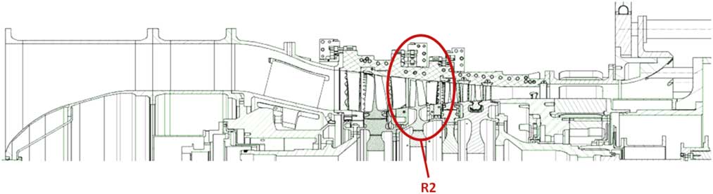
Figure 1 (Colour online) Sectional drawing of Rig 250 Build 6.
In conclusion, forced response analyses are carried out in order to evaluate the impact of differing mistuning distributions. In this regard, the method of aerodynamic influence coefficients (AICs) is employed( Reference Hanamura, Tanaka and Yamaguchi 11 ). AICs are implemented in the SNM models as described by Giersch et al.( Reference Giersch, Hönisch, Beirow and Kühhorn 12 ) in order to consider aeroelastic coupling. It is found that in particular the impact of s/g instrumentation on blade frequencies has to be taken into account since it is significantly influencing the forced response.
2.0 BASIC VIBRATION ANALYSES
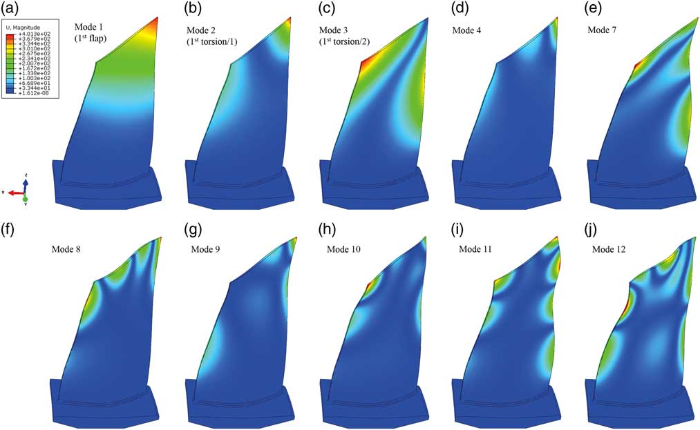
In order to get an idea about the relevant natural frequencies and mode shapes of R2, a finite element sector model composed by tetrahedral elements with 231.000 degrees of freedom (DOF) has been set up considering cyclic symmetry boundary conditions. The nodal diameter plot (Fig. 2) shows 14 coloured horizontal lines representing blade mode families (BFs) in which more than 90% of the strain energy is concentrated in the blades. In particular, this type of mode will be considered in this paper since it is prone to develop localisations in case of the presence of unavoidable mistuning. Figure 3 gives an impression of the blade modes dedicated to the numbering of BF. The black dots in Fig. 2 are mixed modes( Reference Klauke, Kühhorn, Beirow and Golze 13 ), with a clearly higher contribution of the disk motion and hence a smaller level of strain energy in the blades.
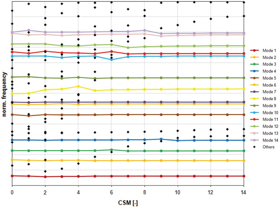
Figure 2 (Colour online) Nodal diameter plot.

Figure 3 (Colour online) Blade mode shapes: (a) 1, (b) 2, (c) 3, (d) 4, (e) 7, (f) 8, (g) 9, (h) 10, (i) 11 and (j) 12.
Assuming free boundary conditions, sector mode shapes and natural frequencies are computed first for the resting blisk. The data are proceeded to build up the SNM models later on, which are valid for one particular BF each and easily allow for a consideration of mistuning described by blade-to-blade frequency deviations as shown in Section 3.1. Furthermore, tremendous reductions in model sizes are achieved in this way. In the best case, the remaining number of DOF is equal to the number of blades.
3.0 STRUCTURAL MISTUNING
3.1 Experimental mistuning identification
The experimental determination of frequency mistuning patterns is accomplished employing blade-by-blade tests, according to a patented approach introduced by Kühhorn and Beirow( Reference Kühhorn and Beirow 14 ). For this purpose, miniature hammer excitation is applied in order to excite each blade of the blisk step by step. Simultaneously the vibration velocity response of the same blade being excited is measured by means of a laser Doppler vibrometry (LDV) in a non-intrusive manner. The hammer itself is held by a retaining fixture and released by means of electromagnetic control, which enables impacts at exactly the same position and with identical intensity (Fig. 4). Free support conditions are chosen for each test. In order to isolate a blade-dominated frequency in the frequency response functions (FRFs), additional mass detuning is employed by putting individual masses on every blade except the one which is currently excited. In this way, the commonly slightly disturbed cyclic symmetry due to mistuning is destroyed completely and modal decoupling of blade-dominated frequencies is achieved by choosing both the quantity and the positioning of the additional mass detuning in a skilful manner depending on the blade mode to be excited. Further efforts are required with regard to finding an ideal position of excitation which usually represents a compromise between the frequency range to be excited, the mode of interest and the flexibility of the blade. In the next step, blade-dominated frequencies have to be read out of the FRFs yielding frequency mistuning distributions that usually differ from mode to mode. Afterwards these mode-individual mistuning patterns are used as input information for updating structural models.
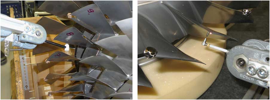
Figure 4 (Colour online) Mistuning ID by means of blade-by-blade tests.
The consideration of s/g in the model-update process is of interest since all blades of the rotor 2 (R2) are instrumented with s/g and it is well known that the s/g instrumentation may significantly affect blade vibration( Reference Beirow, Kühhorn and Nipkau 15 ). Moreover, the influence of assembling all four stages is taken into account. That is why the experimental identification of mistuning is repeated three times, namely:
1. single R2 without s/g instrumentation immediately after fabrication,
2. single R2 with s/g instrumentation and
3. R2 with s/g instrumentation and assembled.
Three different s/g positions are determined by means of a Rolls-Royce in-house s/g positioning tool in order to monitor modes up to a frequency of 12 kHz with a sufficiently high level of signals. Figure 5 indicates the three different positions of s/g, which are distributed in blocks as follows:
1. Position 1 at leading edge (LE) hub applied on blades 1, 4, 7, 10, 13, 16, 19, 22, and 25,
2. Position 2 at trailing edge (TE) mid applied on blades 2, 5, 8, 11, 14, 17, 20, 23, 26, and 28 and
3. Position 3 at LE tip applied on blades 3, 6, 9, 12, 15, 18, 21, 24, and 27.
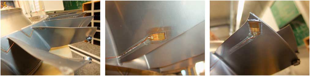
Figure 5 (Colour online) S/g positions: (a) Pos. 1 (LE, hub, left), (b) Pos. 2 (TE, mid) and (c) Pos. 3 (LE, tip, right).
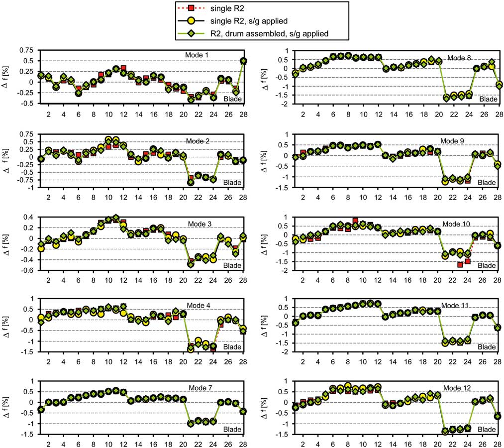
The results of the mistuning tests depicted in Fig. 6 are showing relative frequency deviations for ten different blade modes, according to Equation (1) where index k denotes the kth mode, index i stands for the ith blade (i=1...28):
 $${\rm \Delta }f_{{k,i}} {\equals}{{f_{{k,i}} {\minus}{\rm }\bar{f}_{k} } \over {\bar{f}_{k} }}\,$$

Figure 6 (Colour online) Frequency mistuning patterns derived from test data.
Three main characteristics of the curves are noticeable. First, at least at the first view the differences between the curves of each particular mode hardly seem to be appearing. Second, the mistuning patterns of all modes are revealing clearly decreased magnitudes of blade-dominated frequencies in case of the blades 21, 22, 23 and 24. Within optical geometry measurement carried out at Dresden University( Reference Popig, Hönisch and Kühhorn 16 ), it could be seen that these blades are exposed to strong geometric deviations caused by manufacturing. Later on, Popig et al.( Reference Popig, Hönisch and Kühhorn 16 ) could prove the correlation between geometric deviations and frequency mistuning using a proper orthogonal decomposition (POD)-based approach. Third, although the mistuning strength is different from mode to mode, all frequency mistuning patterns shown in Fig. 6 are taking a similar shape. After assembling, the smallest mistuning strength is determined for Mode 3 (max Δf≈ 0.50%), and the greatest one can be found for Mode 8 (max Δf≈1.71%). Without considering the blades 21–24, the mistuning strength would generally not exceed 1%.
Contrary to the first impression regarding the mode-individual differences in mistuning due to s/g-instrumentation and assembling (Fig. 6), a deeper analysis with respect to percentage differences of blade-dominated frequencies (Equations (2a) and (2b)) clearly indicates a non-negligible impact (Fig. 7):
 $${\rm \Delta \Delta }f_{{k,i}} {\equals}{\rm \Delta }f_{{k,i}}^{{{\rm single},{\rm s}\,/\,{\rm g}}} {\minus}{\rm \Delta }f_{{k,i}}^{{{\rm single},{\rm without}\,{\rm s}\,/\,{\rm g}}} \,$$
 $$\hskip -8pt{\rm \Delta \Delta }f_{{k,i}} {\equals}{\rm \Delta }f_{{k,i}}^{{{\rm assembled},{\rm s}\,/\,{\rm g}}} {\minus}{\rm \Delta }f_{{k,i}}^{{{\rm single},\,{\rm s}\,/\,{\rm g}}} \,\, $$

Figure 7 (Colour online) Percentage difference in blade-dominated frequencies of (a) single R2 without s/g and (b) assembled R2 with s/g compared to the results of single R2 with s/g-instrumentation.
The distributions of ΔΔf take local minimum values at blades 3, 6, 9, 12, 18, 21, 24 and 27 for modes 1, 2, 3 and 7 (Fig. 7a), i.e. those blades applied with s/g at position 3. This can be explained by both the impact of s/g mass located at position 3 at the tip and a possible stiffness contribution of s/g located at positions 2 and 3 closer to the hub. In contrast, the mistuning patterns of mode 11 almost consistently indicate local minima at blades 1, 4, 7, 10, 13, 16, 19, 22 and 25, which are instrumented with a s/g at position 1 (LE, hub) each. Again this can be explained by the mass contributions of these s/g, each positioned at a vibration antinode of mode 11 (Fig. 3i).
In the worst case, the total change in blade-dominated frequencies caused by s/g instrumentation is ranging between –0.21% and +0.24% (Mode 2; Fig. 7a). Since this is not far away from the typical frequency mistuning bands with a standard deviation of about 0.3% found for milled HPC Blisks( Reference Figaschwsky and Kühhorn 4 ), a noticeable impact with respect to the forced response is most likely if modal damping ratios are small. Further deviations without distinct tendency become apparent due to assembling (Fig. 7b). Hence, three different structural models are updated based on the measured mistuning data for each mode of interest with a view to analysing the impact of mistuning induced by s/g application and assembling.
3.2 Model update
The experimental mistuning data are processed in order to update the structural models. For that purpose, the SNM models have been chosen, which have to be individually updated for every frequency mistuning pattern being experimentally determined. In this regard, it is a well-established technique to adjust the Young’s modulus of each blade according to the measured distributions of relative blade-dominated frequency deviations depicted in the previous section( Reference Hönisch, Kühhorn and Beirow 17 ). Assuming that
 $$f_{{k,i}} \,\sim\,\sqrt {E_{{k,i}} } ,$$
which directly results from the solution of Kirchhoff plate’s differential equation. The connectivity between deviations of blade-dominated frequencies and blade Young’s modules of blade i and BF k can be approximated by
 $${\rm \Delta }f_{{k,i}} \,\approx\,{1 \over 2}{\rm \Delta }E_{{k,i}} \,$$
Correction of the possible mean frequency shifts is provided by an additional adjustment of the global structural density. This latter adjustment becomes necessary since the regular material properties used in the underlying FE model commonly do not match exactly with the real material properties. Thus, numerically and experimentally determined BF frequency mean values are reconciled. Since the SNM are modal models, they are well suited for forced response computations in terms of displacements, which is the focus here with respect to reliable assessments of BTT data later on. A validation of the SNM models is provided in Section 4.2 by comparing mode shapes of the models with those derived from experimental modal analyses carried out at stationary conditions. In respect of later evaluations of BTT data, the impact of rotational speed and the relevant temperature field on natural frequencies will be taken into account afterwards.
4.0 EXPERIMENTAL MODAL ANALYSES
4.1 Modal damping ratios and natural frequencies
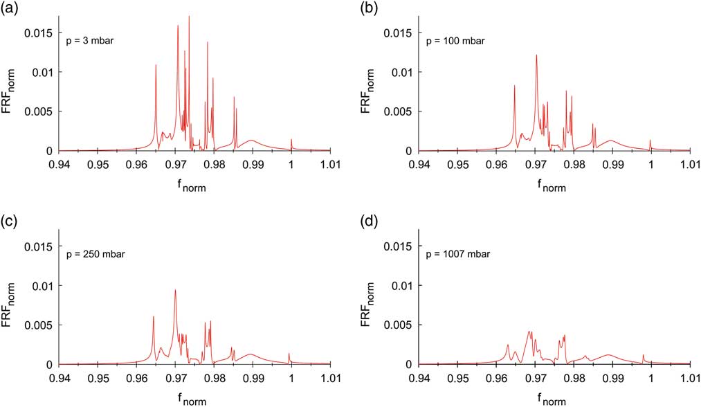
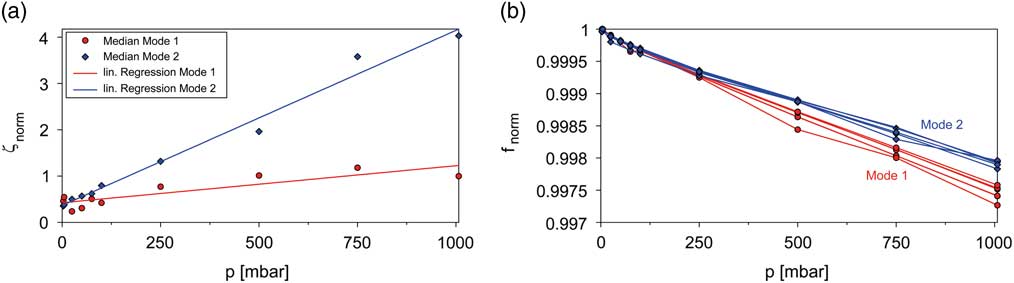
Since blisk designs suffer from an extreme low mechanical damping level, its accurate knowledge is highly important for surge event simulations. Furthermore, one would benefit from a validation of the dominating aerodynamic damping part considered via AIC in case of forced response analyses. That is why additional experimental modal analyses have been carried out inside a pressure vessel for the single blisk without s/g-instrumentation employing piezoelectric excitation at the stationary blisk and LDV response measurement at the LE tip of each blade to identify the damping contributed by the ambient air and its dependence on the air density (Fig. 8). The piezoelectric disc element is applied with glue to the inner disk rim (detail in Fig. 8). Due to the positioning at the disk and the low weight of the piezo (3.6 g), modal properties are hardly affected. The soft suspension of the blisk most closely corresponds to free support conditions, so that elusive effects on modal quantities resulting from a possible clamping of the structure are minimised. In this way, numerous FRF could be determined, allowing for an identification of modal ratios using a multi degree of freedom (MDOF) fit approach as introduced in Ref. Reference Beirow, Maywald, Figaschewsky, Kühhorn, Heinrich and Giersch18. Figure 9 clearly indicates an increasing level of modal coupling with increasing ambient pressure; and hence, the best separation of peaks is appearing at 3 mbar. Furthermore, it becomes apparent that starting at technical vacuum (3 mbar, 20°C), an approximately linear increase in modal damping ratios could be identified with increasing air density up to 1,007 mbar (at 20°C). The analyses are focused on BFs 1 and 2 for which differing gradients have been detected (Fig. 10a). Please note that the regression curves plotted in the figure are based on median values computed from modal damping ratios of different modified cyclic symmetry modes. Close to technical vacuum, the medians of modal damping ratios take minimum values of roughly the same magnitude for both BFs. Since the impact of ambient air is negligible for this particular case, one can interpret the damping ratios found as pure structural damping. Compared to technical vacuum, approximately 3 times (BF 1) or even 11 times (BF 2) greater values are determined at 1,007 mbar. The large differences seem to be surprising; however, they can be explained with the impact of acoustic reflections between adjacent blades, which are more significant for modes emitting acoustic waves with a large wave length, as it is the case for a Mode 1 blade motion.
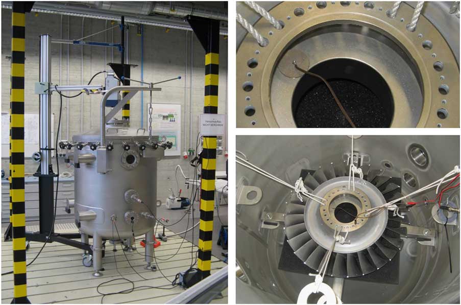
Figure 8 (Colour online) R2 inside the pressure vessel.

Figure 9 (Colour online) Normalised FRF at different pressure (BF 2).

Figure 10 (Colour online) (a) Normalised modal damping ratios and (b) normalised natural frequencies of BF 1 and 2.
It could be shown in foregoing publications( Reference Beirow, Maywald, Figaschewsky, Kühhorn, Heinrich and Giersch 18 , Reference Figaschewsky, Kühhorn, Beirow, Giersch, Nipkau and Meinl 19 ) that damping results generated in the manner indicated before represent a satisfying approximation for operational conditions in case of higher blade modes and sufficiently large distances from blade to blade. Two rotating test cases were considered in Ref. Reference Figaschewsky, Kühhorn, Beirow, Giersch, Nipkau and Meinl19, an axial high-pressure compressor blisk and a radial turbine impeller. In both cases, the damping information in operation could be obtained from s/g-data employing MDOF fit approaches. A remarkable match with the damping estimated at rest could be found, if both high vibration frequencies and high inlet Mach numbers are present and, if acoustic radiation can be regarded as major damping source (e.g. as given for BF 11 of the rotor considered in this paper). In case of low vibration frequencies, e.g. as given for fundamental blade modes (e.g. BF 1 and 2), other aerodynamic damping mechanisms are dominating, and no agreement with test results at stationary conditions could be found.
Due to an increasing effect of co-vibrating air mass with increasing air pressure, the natural frequencies are generally decreasing in a linear manner (Fig. 10b). A slightly stronger decline becomes apparent for BF 1, which can be explained with a more planar shape characteristic compared to BF 2 (Fig. 2) and hence, a stronger impact of air mass. Multiple Mode 1 and 2 lines are representing the small differences arising for a selection of low-order modified cyclic symmetry mode (MCSMs; Fig. 10b).
4.2 Mode shapes and model validation
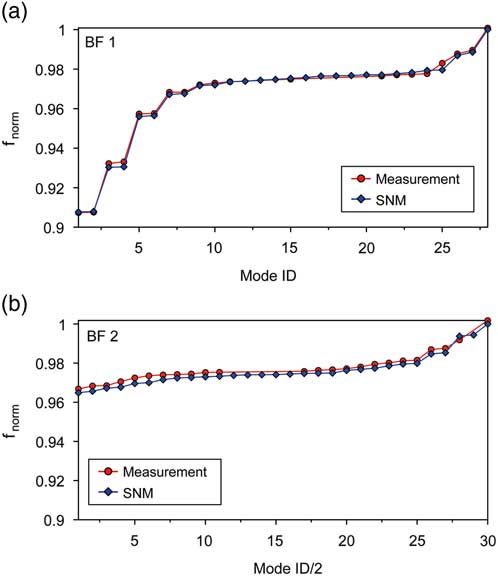
Aiming at a model validation in terms of natural frequencies, the best possible separation of peaks is advantageous as it is achieved within the experiments carried out at technical vacuum. According to the previous section, necessary FRFs are only available for BF 1 and BF 2 of the single R2 without s/g. Figure 11 shows the numerical results of normalised natural frequencies being computed by updated SNMs in comparison with experimentally determined data. Please note that apart from adjusting the blade-to-blade stiffness, a global adaption of material density has been employed. The good agreement of the curves emphasises the quality of the SNM models with regard to both the absolute values and the shape of the curves. Missing red dots in Fig. 11 indicate that some of the natural frequencies could not be determined experimentally, e.g. because they were hardly excited within the measurement campaign. In comparison with BF 2, which is dedicated to blade torsion, a greater spreading of normalised frequencies becomes apparent with BF 1 representing the first blade flap mode. This indicates a stronger modal coupling among disk and blade motion for Mode ID 1–6 (f norm<0.96).

Figure 11 (Colour online) Mistuned natural frequencies, measurement versus computation with updated numerical models (a) BF 1 and (b) BF 2.
Due to the lack of further data at technical vacuum, continuative validations are based on experimental results obtained under normal conditions for the single blisk with s/g instrumentation. These validations are focused on unwrapped mode shapes measured at the LE tip in axial direction. An exemplary selection of results is shown in Figs 12 and 13 (red curves) for different BFs, which contain both approximately regular modes denoted as MCSMs and localised mode shapes as a typical result of mistuning. An increased level of deflections is noticeable for a number of modes at blades 21–24, e.g. MCSM0, which is directly correlated with the geometric deviations of these blades mentioned in Section 3( Reference Popig, Hönisch and Kühhorn 16 ). In addition, dedicated modes calculated with the updated SNM models are plotted in the diagrams (blue curves), which are showing a largely satisfying match between numerical and experimental results.
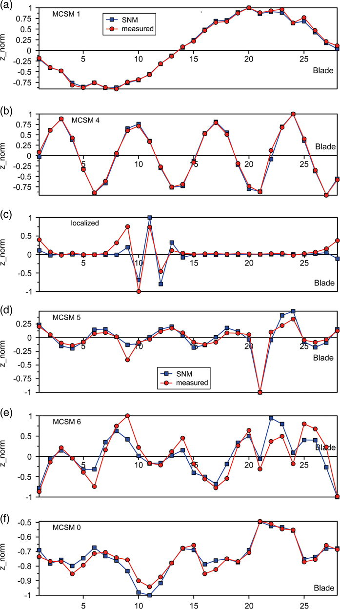
Figure 12 (Colour online) (A) Mode shapes for BF 1 (a–c) single R2 with s/g and (B) Mode shapes for BF 2 (d–f), single R2 with s/g.
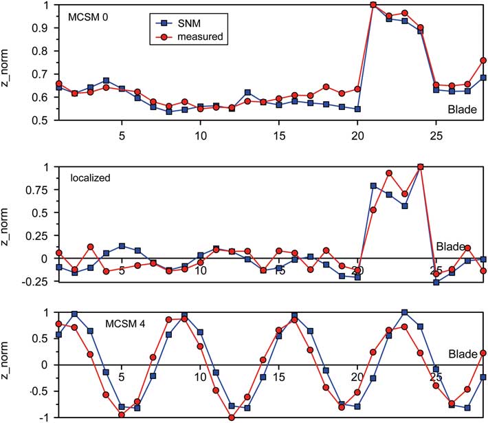
Figure 13 (Colour online) Mode shapes for BF 11, single R2 with s/g.
5.0 FORCED RESPONSE ANALYSES
Exemplary forced response analyses in terms of rotating engine order (EO) excitations are carried out on the one hand to investigate the effect of changing mistuning due to s/g instrumentation and assembling. On the other hand, the reliability of the SNM is checked for one case, which could be detected within the rig test campaign: an EO 4 excitation (difference of upstream inlet guide vane and Stator 1( Reference Beirow, Kühhorn, Figaschewsky, Hönisch, Giersch and Schrape 21 )) of the 1F mode at 81% speed causing a response dominated by travelling wave modes (TWMs) 4 and –9. A Campbell diagram is provided in Ref. 10. It is important to mention that the SNM has to be adjusted with respect to operational conditions to consider the impact of rotational speed and relevant temperature field. Hence, additional FE analyses have been carried out to provide the necessary modal information for SNM adjustment.
Aeroelastic effects are taken into account by employing the AIC technique. The determination of AIC requires a computational fluid dynamics simulation of a simple blade cascade for instance. Stationary flow conditions are initially assumed corresponding to the operational point considered. Following this, the flow field is disturbed by forcing one reference blade of the cascade to perform a sine-shaped motion in a particular mode shape. In consequence, pressure fluctuations or modal forces, respectively, are acting on each blade of the cascade. Finally, the AICs are determined by means of dividing modal forces by the maximum modal displacement of the reference blade. Then the AICs are implemented into a circular AIC matrix, from which an impedance matrix Z is computed by transformation from blade individual co-ordinates into travelling wave co-ordinates. The impedance matrix multiplied with the vector of modal displacement represents the motion-induced forcing of one particular point of operation to be considered in the SNM model( Reference Giersch, Hönisch, Beirow and Kühhorn 12 ), as given in the following equation:
 $$\left[ {{\minus}{\rm \Omega }^{2} M{\plus}j{\rm \Omega }{\mib{D}} {\plus}{\mib{K}} {\plus}{\rm \Delta }{\mib{K}} {\plus}{\mib{Z}} } \right]{\mib{q}} \left( {j{\rm \Omega }} \right){\equals}{\mib{F}} $$
Since mass-normalised mode shapes have been processed, the modal mass matrix M equals to the unit matrix. D represents the matrix of modal structural damping, K the modal stiffness matrix of the tuned reference including centrifugal and temperature effects, whereas the matrix Δ K is taking into account the mistuning information by means of sector stiffness deviations. F stands for the vector of external modal forcing and q for the vector of modal displacements.
Figure 14 indicates the greatest magnifications γ due to a pure EO 4 excitation of the mistuned blisk compared to its tuned counterpart, max γ takes a value of 1.18 at blade 27 (assembly, with s/g). For the single blisk, the greatest magnification is slightly lesser with 1.16 (with s/g) but 1.11 without s/g instrumentation. Generally, the largest differences between the mistuned responses are caused by the s/g instrumentation while the impact of assembling hardly affects the response, which is in agreement with the findings published by Klauke et al.( Reference Klauke, Kühhorn, Beirow and Parchem 20 ).
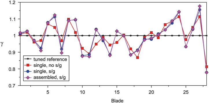
Figure 14 (Colour online) Maximum displacement magnification due to mistuning (BF1, EO 4).
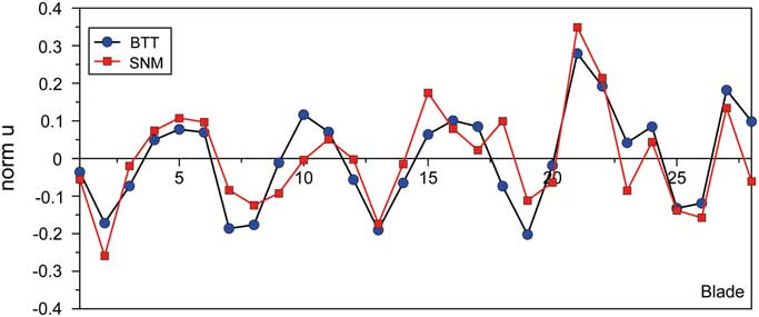
The good quality of the SNM models has been already proved for the blisk at rest in Section 4.2. With regard to the rotating blisk, both s/g and BTT data have been gathered in the rig test campaign mentioned before. Consequently, a basis of validation data is available. In Fig. 15, one example of a BTT shot response in terms of a normalised displacement is revealed in comparison with an SNM computation. In this particular case, an EO 4 excitation yielding a response dominated by the TWMs 4 and –9 could be identified by evaluating the BTT data. That is why apart from the dominating TWM 4 excitation, an additional phase-lagged forcing of TWM –9 is considered in the SNM, which is iteratively adjusted in both phase and amplitude in order to achieve the best match with the BTT results. Although deviations become evident in detail, the overall shape of the BTT curve is basically confirmed by the SNM in a satisfying manner. Hence, the suitability of the SNM to compute the forced response close to reality is demonstrated in principle at least for one example. Further enhancements could be achieved by taking into account gyroscopic effects and the impact of adjacent rotors. For a continuative and deeper assessment of data addressing the last mentioned topics and the validity of the structural models, please refer to the work of Figaschewsky et al.( Reference Figaschewsky, Kühhorn, Beirow, Schrape and Giersch 10 ).

Figure 15 (Colour online) Normalised maximum blade displacement (BF 1, mixed TWM 4/–9 response due to an EO 4 excitation).
6.0 CONCLUSIONS
Aiming to prepare for an accurate evaluation of BTT rig test data, comprehensive preliminary experimental analyses of HPC blisk mistuning have been carried out to understand the consequences of s/g instrumentation and assembling on mistuning. More specifically blade-by-blade tests have been accomplished, yielding frequency mistuning patterns up to blade mode 11. Although the patterns found are similar at first appearance, the differences from blade to blade and state of construction are substantially caused by the s/g instrumentation. Depending on s/g position and the particular blade mode, either the mass or the stiffness contribution of the s/g noticeably changes the blade frequencies, whereas the impact of assembling is negligible. The experimentally determined mistuning patterns have been used to update SNM models, which could be validated by comparing both natural frequencies and mode shapes of numerical and experimental modal analyses determined for the blisk at rest.
It could be confirmed within forced response analyses for BF 1 at operational conditions that again the s/g instrumentation noticeably affects the results, whereas the impact of assembling hardly carries weight. Finally, an example is considered which shows that the BF 1 SNM model is well suited to recalculate the displacement response of a BTT shot gathered during a rig test.
ACKNOWLEDGEMENTS
The work presented herein has been supported by the Rolls-Royce Deutschland company and the German Aerospace Center (DLR) as well. The authors thank for this commitment. The independent investigations contribute to the research project ‘AeRoBlisk (Subproject: Robust Blisk Blade Design)’ with a funding by the German Federal Ministry of Economics and Technology. The original work underlying the present paper was issued in the proceedings of ISABE 2017conference( Reference Beirow, Kühhorn, Figaschewsky, Hönisch, Giersch and Schrape 21 ).