


NOMENCLATURE
- β
-
angle between the limiting and external streamline
- c
-
chord along the line of flight
- cE
-
entrainment coefficient used in Head's method(Reference Head1)
- δ
-
boundary layer thickness
- δ 1, δ 2
-
boundary layer displacement thicknesses
- η
-
spanwise coordinate (colinear with y direction)
- θ 11, θ 12, θ 21, θ 22
-
boundary layer momentum thicknesses
- f 1, f 2, f 3, f 4
-
scaling factors relating crossflow integral length scales, defined in the appendix
- H
-
boundary layer shape factor, H = δ 1 / θ 11
- H 1
-
entrainment shape factor, H 1 = (δ - δ 1) / θ 11
- k
-
von Kármán's constant from universal log-law
- κ T
-
curvature of conical arc normal to generators of a swept-tapered wing, κ T = 1/r
- Λ
-
local sweep angle between line-of-flight coordinate ξ and spanwise coordinate η
- Rθ
-
Reynolds number based on momentum thickness
- r
-
radius of curvature of conical arc normal to generators of a swept-tapered wing
- σ
-
shorthand for sinψ tanβ
- τ0
-
wall shear stress
- Ue
-
velocity of the inviscid flow at the edge of boundary layer
- U 1
-
component of Ue parallel to the x direction
- u
-
component of boundary layer velocity parallel to external streamline
- u+
-
boundary layer velocity parallel to external streamline in wall units, u+ = u/(Ue √(cf /2))
- V 1
-
component of Ue parallel to the y direction
- v
-
component of boundary layer velocity normal to external streamline
- x
-
conical coordinate normal to the direction of the wing generators
- ξ
-
line-of-flight coordinate
- y
-
conical coordinate parallel to the direction of the wing generators
- z
-
wall normal coordinate
- z+
-
normalised wall normal coordinate, z+= (Ue z / υ) √(cf /2)
- υ
-
kinematic viscosity
- ψ
-
angle between inviscid streamline and x coordinate, ψ=tan–1 (V 1/U 1)
1.0 INTRODUCTION
For transport aircraft wings operating at high Reynolds numbers, the flow along the Attachment Line (AL) is often turbulent, and numerical methods, including low-order Computational Fluid Dynamics (CFD) codes, need to be able to predict the development of the wing boundary layer flow starting from a turbulent AL. An example of such an application is the recent Airbus study undertaken by Alderman et al(Reference Alderman, Rolston, Gaster and Atkin2) on the control of attachment line transition using a turbulent contamination avoidance device. In contrast to an unswept wing, the presence of a spanwise velocity component introduces large curvature in the inviscid streamline as the flow is turned from the spanwise direction at the AL towards the chordwise direction by the acceleration normal to the Leading Edge (LE) as shown schematically in Fig. 1. Modelling the flow in the vicinity of the AL poses significant challenges due to the presence of highly curved streamlines and possibly large turbulence anisotropy arising from the rapidly changing shear strain.

Figure 1. Schematic representation of the flow along a swept wing.
Recent years have seen complex-topology Reynolds-Averaged Navier–Stokes (RANS) codes displace the lower-fidelity methods which formed the mainstay of the wing design process during the 1980s and 1990s. However, there is renewed interest in low-order CFD as a replacement for simple data-sheet methods in the conceptual/preliminary design phases, particularly when flow control schemes are being considered. One such method is the Airbus Callisto code, a turbulent boundary layer method based on the von Kármán momentum integral equations, incorporating the lag-entrainment model of Green et al(Reference Green, Weeks and Brooman3), and modelling three-dimensional turbulence using the streamline analogy. The coupling of boundary layer analysis with inviscid field analysis for attached and weakly separated flows is described in detail by Lock and Williams(Reference Lock and Williams4), and has the advantage of requiring considerably less computing resource than RANS, with comparable accuracy for attached flows, while simplifying the isolation of the profile drag component of a wing.
The rationale behind the Callisto development was to develop a lag-entrainment code which could be coupled to many different inviscid solvers, and indeed to develop an Object-Oriented (OO) coupling framework which could be exploited by other boundary layer methods. Callisto has now been coupled to a wide range of codes: the BAE Systems code RANSMB (structured multi-block) and Flite3D (unstructured Euler); Fluent, via user-defined functions; and the DLR TAU-Code. The method is accessed by the inviscid solvers as a shared object library; this software architecture means that the same modelling, implemented via the same lines of code, is accessed by each solver. As well as meeting the reusability objective for OO software, this approach simplifies the transfer of novel flow-physics models (e.g., laminar flow control) from research-type to industrial methods with some confidence. In order to permit rapid conceptual flow control studies on transonic wing geometries, Callisto has also been coupled to the full potential aerofoil method of Garabedian and Korn(Reference Garabedian and Korn5), extended to handle infinite-swept and swept-tapered wing flows using Lock's transformation(Reference Lock6). Callisto Viscous Garabedian and Korn, or CVGK, is therefore a 2½D version of the BVGK method developed at the Royal Aircraft Establishment (RAE)(Reference Ashill, Wood and Weeks7). A recent numerical study conducted by Atkin and Gowree(Reference Atkin and Gowree8) demonstrated that CVGK can predict the drag on swept wings in transonic flow with good accuracy.
In the case of the turbulent AL, the streamline analogy leads to ill-posed governing equations in a very confined region downstream of the AL where the streamline direction is more or less perpendicular to the marching direction of the boundary layer solver. The singularity at the AL itself is resolved by invoking local similarity arguments, but immediately downstream of the AL, there are lingering robustness issues which seemingly cannot be resolved. In Callisto, this region has to date been approximated by simply extrapolating the results of the AL calculation over the first 0.5% or so of wing chord.
Due to the lack of detailed measurements in this region, it is difficult to benchmark this approximation or to derive a more reliable semi-empirical model for the turbulence. The lack of good data for a turbulent boundary layer at the LE of a swept wing may be explained by the topological complexity of the three-dimensional (3D) boundary layer, which also tends to be very thin at its origin and growing very slowly due to the presence of a favourable pressure gradient. An experimental campaign was therefore conducted to investigate the behaviour of the viscous flow in the vicinity of the AL generated on a wing model with very high LE sweep so as to validate and, if possible, improve the near-attachment flow modelling in Callisto and related boundary layer codes.
The layout of this paper is as follows. Section 2 contains a description of the numerical modelling, comprising the governing equations and the approximation to these at the leading edge to overcome numerical issues. In Section 3, a brief description of the experiment is presented; more detail of the hot-wire and optical alignment system can be found in Gowree et al(Reference Gowree, Atkin and Grupppetta9), together with an analysis of the accuracy of the measurements. The experimental results are presented in Section 4 and, based on the new insight from these findings, the governing equations were modified for the region of the flow immediately downstream of the attachment line. These modifications are presented in Section 5 along with a comparison of the old and new approached with the new experimental results. The paper concludes with a discussion of both experimental trends and numerical modelling and a summary of the contribution to the body of knowledge.
2.0. NUMERICAL MODELLING IN CALLISTO
2.1 Coordinate system
The idealised geometry used by 2½D methods to model swept-tapered wings is illustrated in Fig. 2. The wing is assumed to be of constant section and twist, with leading and trailing edges meeting at a point O. All radii r joining the origin O with a point on the wing surface are generators of that surface. This conical symmetry is assumed to extend to the external inviscid flowfield such that isobars of surface pressure are coincident with the wing generators.

Figure 2. Schematic of a swept-tapered wing illustrating the line-of-flight section AB and the undeveloped computational arc AC for the boundary layer calculation.
Both the magnitude and the direction of the inviscid flow at the boundary layer edge are assumed to be independent of spanwise position. This allows the variation of the viscous flowfield with spanwise position to be reduced to a simple length scale dependence: in laminar boundary layer theory, the boundary layer thickness can be shown to vary with r ½(Reference Kaups and Cebeci10,Reference Horton and Stock11) , while for turbulent boundary layers, the integral length scale varies more or less as r (Reference Ashill and Smith12). To simplify reduction of the governing equations to infinite-yawed-wing form as the local taper radius r tends to infinity, a taper curvature κT is used.
2.2 Governing equations
Although based upon a well-established theory, the integral boundary layer equations within Callisto have been developed and refined over a number of years, starting with the entrainment method of Head(Reference Head1), which added to the classical von Kármán equation a transport equation for the boundary layer shape factor, H. Green(Reference Green13) extended Head's method to compressible flows by means of a transformed shape factor H , defined in Equation (6), and then introduced the effects of turbulence history by adding an equation to account for the lag in the response of the turbulence to changes in the strain field(Reference Green, Weeks and Brooman3). At the same time, Smith(Reference Smith14) extended the basic approach to three-dimensional flows by employing the streamline analogy, whereby turbulence characteristics in a 2D boundary layer are assumed to be replicated by the flow resolved the direction of the external streamline in a 3D boundary layer: closure of the increasing number of momentum thicknesses is achieved by assuming functional dependence of those length scales upon the streamwise momentum thickness, θ11 , the transformed shape factor H , and the twist β of the limiting streamline (at the wall) relative to the direction of the inviscid flow. Smith's fully 3D approach was adapted for the special case of swept-tapered wings described above by Ashill and Smith(Reference Ashill and Smith12), to provide a low-cost approach to assessing the effect of sweep and taper on turbulent boundary layers on transonic wings. The advantages of lower-cost, approximate methods are still evident today where they can be enablers for CPU-intensive optimization strategies.
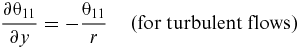
The governing equations in the Callisto code are derived from the system of three integral equations for momentum, resolved parallel and normal to the inviscid flow streamline, and for entrainment, as presented by Ashill and Smith(Reference Ashill and Smith12). The latter system of equations is presented in the appendix, as are the principal modifications to the notation and to the choice of independent variables adopted for the Callisto method. The resulting system, expressed in the conical-surface (x,y) coordinate system illustrated in Fig. 2, can be written:
 $$\begin{equation}
\left( {\begin{array}{@{}*{3}{c}@{}} {{A_\theta }}&\ {{A_\beta }}&\ {{A_{\bar{H}}}}\\ {{N_\theta }}&{{N_\beta }}&{{N_{\bar{H}}}}\\ {{E_\theta }}&{{E_\beta }}&{{E_{\bar{H}}}} \end{array}} \right)\frac{d}{{dx}}\left( {\begin{array}{@{}*{1}{c}@{}} {{\theta _{11}}}\\ {\tan \beta }\\ {\bar{H}} \end{array}} \right) = \;\left( {\begin{array}{@{}*{1}{c}@{}} {{\lambda _1}}\\ {{\lambda _2}}\\ {{\lambda _3}} \end{array}} \right)
\end{equation}$$
$$\begin{equation}
\left( {\begin{array}{@{}*{3}{c}@{}} {{A_\theta }}&\ {{A_\beta }}&\ {{A_{\bar{H}}}}\\ {{N_\theta }}&{{N_\beta }}&{{N_{\bar{H}}}}\\ {{E_\theta }}&{{E_\beta }}&{{E_{\bar{H}}}} \end{array}} \right)\frac{d}{{dx}}\left( {\begin{array}{@{}*{1}{c}@{}} {{\theta _{11}}}\\ {\tan \beta }\\ {\bar{H}} \end{array}} \right) = \;\left( {\begin{array}{@{}*{1}{c}@{}} {{\lambda _1}}\\ {{\lambda _2}}\\ {{\lambda _3}} \end{array}} \right)
\end{equation}$$
and
 $$\begin{equation}
\frac{{\partial {\theta _{11}}}}{{\partial y}} = - \frac{{{\theta _{11}}}}{r}\quad \left( {{\rm{for\ turbulent\ flows}}} \right)\\
\end{equation}$$
$$\begin{equation}
\frac{{\partial {\theta _{11}}}}{{\partial y}} = - \frac{{{\theta _{11}}}}{r}\quad \left( {{\rm{for\ turbulent\ flows}}} \right)\\
\end{equation}$$
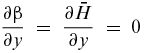 $$\begin{equation}
\frac{{\partial \beta }}{{\partial y}}\; = \;\frac{{\partial \bar{H}}}{{\partial y}}\; = \;0
\end{equation}$$
$$\begin{equation}
\frac{{\partial \beta }}{{\partial y}}\; = \;\frac{{\partial \bar{H}}}{{\partial y}}\; = \;0
\end{equation}$$
The non-trivial coefficients Am and λʹn are defined in the appendix. The independent variables in the above equations relate to the 3D boundary layer profiles as follows:
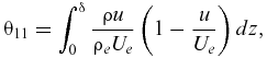 $$\begin{equation}
{\theta _{11}} = \int_0^\delta {\frac{{\rho u}}{{{\rho _e}{U_e}}}\left( {1 - \frac{u}{{{U_e}}}} \right)dz} ,\\
\end{equation}$$
$$\begin{equation}
{\theta _{11}} = \int_0^\delta {\frac{{\rho u}}{{{\rho _e}{U_e}}}\left( {1 - \frac{u}{{{U_e}}}} \right)dz} ,\\
\end{equation}$$
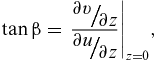 $$\begin{equation}
\tan \beta = {\left. {\frac{{{\raise0.7ex\hbox{${\partial v}$} \!
/ \!\lower0.7ex\hbox{${\partial z}$}}}}{{{\raise0.7ex\hbox{${\partial u}$} \!
/ \!\lower0.7ex\hbox{${\partial z}$}}}}} \right|_{z = 0}},\\
\end{equation}$$
$$\begin{equation}
\tan \beta = {\left. {\frac{{{\raise0.7ex\hbox{${\partial v}$} \!
/ \!\lower0.7ex\hbox{${\partial z}$}}}}{{{\raise0.7ex\hbox{${\partial u}$} \!
/ \!\lower0.7ex\hbox{${\partial z}$}}}}} \right|_{z = 0}},\\
\end{equation}$$
 $$\begin{equation}
\bar{H} = \frac{1}{{{\theta _{11}}}}\int_0^\delta {\frac{\rho }{{{\rho _e}}}\left( {1 - \frac{u}{{{U_e}}}} \right)dz}
\end{equation}$$
$$\begin{equation}
\bar{H} = \frac{1}{{{\theta _{11}}}}\int_0^\delta {\frac{\rho }{{{\rho _e}}}\left( {1 - \frac{u}{{{U_e}}}} \right)dz}
\end{equation}$$
For completeness, we note that the system of equations above can be solved only for attached flows and that, for flows near to separation or mildly separated, the inviscid velocity gradient becomes an independent variable (rather than a constant factor in the coefficients λ 1, λ 2 and λ 3) governed by an additional equation for the wall-normal velocity at the edge of the boundary layer. The principles of the approach are well described by Lock and Williams(Reference Lock and Williams4); however for the purposes of this paper, the basic three-equation system is sufficient to calculate the development of a turbulent boundary layer near the AL. We also note here that the entrainment equation can be augmented by Green's lag equation but again, as it is not central to the behaviour of the three-equation system at the AL, it will not be discussed in this paper. One further complication is that the governing equations in Callisto are transformed into a non-orthogonal coordinate system, (ξ,η) in Fig. 2. However, the additional terms do not alter the numerical challenge at the leading edge and so again are not introduced in this paper. Rearranging Equation (1) above, and substituting the expressions listed in the appendix, we obtain the first-order, non-linear differential system:
 $$\begin{equation*}
\frac{d}{{dx}}\left( {\begin{array}{@{}*{1}{c}@{}} {{\theta _{11}}}\\ {\tan \beta }\\ {\bar{H}} \end{array}} \right) = {\left( {\begin{array}{@{}*{3}{c}@{}} {\cos \psi - \sigma \,{f_2}}&{ - \sin \psi \,{f_2}{\theta _{11}}}&{ - \sigma \,\frac{{d{f_2}}}{{d\bar{H}}}{\theta _{11}}}\\[6pt] {\tan \beta \left( {\cos \psi \,{f_1} - \sigma \,{f_4}} \right)}&\quad {\left( {\cos \psi \,{f_1} - 2\sigma \,{f_4}} \right)\,{\theta _{11}}}&\quad {\tan \beta \left( {\cos \psi \frac{{d{f_1}}}{{d\bar{H}}} - \sigma \,\frac{{d{f_4}}}{{d\bar{H}}}} \right){\theta _{11}}}\\[6pt] {\cos \psi \,{H_1} + \sigma \,{f_3}}&{\sin \psi \,{f_3}{\theta _{11}}}&{\left( {\cos \psi \frac{{d{H_1}}}{{d\bar{H}}} + \sigma \,\frac{{d{f_3}}}{{d\bar{H}}}} \right){\theta _{11}}} \end{array}} \right)^{ - 1}}\;\left( {\begin{array}{@{}*{1}{c}@{}} {{\lambda _1}}\\ {{\lambda _2}}\\ {{\lambda _3}} \end{array}} \right),
\end{equation*}$$
$$\begin{equation*}
\frac{d}{{dx}}\left( {\begin{array}{@{}*{1}{c}@{}} {{\theta _{11}}}\\ {\tan \beta }\\ {\bar{H}} \end{array}} \right) = {\left( {\begin{array}{@{}*{3}{c}@{}} {\cos \psi - \sigma \,{f_2}}&{ - \sin \psi \,{f_2}{\theta _{11}}}&{ - \sigma \,\frac{{d{f_2}}}{{d\bar{H}}}{\theta _{11}}}\\[6pt] {\tan \beta \left( {\cos \psi \,{f_1} - \sigma \,{f_4}} \right)}&\quad {\left( {\cos \psi \,{f_1} - 2\sigma \,{f_4}} \right)\,{\theta _{11}}}&\quad {\tan \beta \left( {\cos \psi \frac{{d{f_1}}}{{d\bar{H}}} - \sigma \,\frac{{d{f_4}}}{{d\bar{H}}}} \right){\theta _{11}}}\\[6pt] {\cos \psi \,{H_1} + \sigma \,{f_3}}&{\sin \psi \,{f_3}{\theta _{11}}}&{\left( {\cos \psi \frac{{d{H_1}}}{{d\bar{H}}} + \sigma \,\frac{{d{f_3}}}{{d\bar{H}}}} \right){\theta _{11}}} \end{array}} \right)^{ - 1}}\;\left( {\begin{array}{@{}*{1}{c}@{}} {{\lambda _1}}\\ {{\lambda _2}}\\ {{\lambda _3}} \end{array}} \right),
\end{equation*}$$
where we have introduced the shorthand
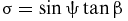 $$\begin{equation}
\sigma = \sin \psi \tan \beta
\end{equation}$$
$$\begin{equation}
\sigma = \sin \psi \tan \beta
\end{equation}$$
This type of initial-value problem is well suited to solution by a Runge-Kutta scheme: the variant due to England(Reference England15), with a facility to reduce the marching step size if the estimated truncation error exceeds a pre-defined threshold, is used in Callisto.
2.3 Conditions for singularity of the viscous derivatives matrix
There are two conditions where the system of Equation (7) can clearly be seen to become singular. The first is most clearly evident in case of 2D flow where tanβ ≡ 0, cosψ ≡ 1 and sinψ ≡ 0 for all x (so that σ ≡ 0), when the normal momentum equation can be de-coupled from the rest of the system, leaving the following equation:
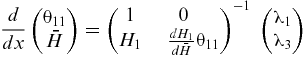 $$\begin{equation}
\frac{d}{{dx}}\left( {\begin{array}{@{}*{1}{c}@{}} {{\theta _{11}}}\\ {\bar{H}} \end{array}} \right) = {\left( {\begin{array}{@{}*{2}{c}@{}} 1&0\\ {{H_1}}&\quad{\frac{{d{H_1}}}{{d\bar{H}}}{\theta _{11}}} \end{array}} \right)^{ - 1}}\;\left( {\begin{array}{@{}*{1}{c}@{}} {{\lambda _1}}\\ {{\lambda _3}} \end{array}} \right)
\end{equation}$$
$$\begin{equation}
\frac{d}{{dx}}\left( {\begin{array}{@{}*{1}{c}@{}} {{\theta _{11}}}\\ {\bar{H}} \end{array}} \right) = {\left( {\begin{array}{@{}*{2}{c}@{}} 1&0\\ {{H_1}}&\quad{\frac{{d{H_1}}}{{d\bar{H}}}{\theta _{11}}} \end{array}} \right)^{ - 1}}\;\left( {\begin{array}{@{}*{1}{c}@{}} {{\lambda _1}}\\ {{\lambda _3}} \end{array}} \right)
\end{equation}$$
The singularity occurs when the parameter
 $\frac{{d{H_1}}}{{d\bar{H}}}$
in Equation (9) becomes zero (at separation). This condition is well known and is dealt with by introducing a transpiration equation to the system and by changing the dependent variables, as discussed above.
$\frac{{d{H_1}}}{{d\bar{H}}}$
in Equation (9) becomes zero (at separation). This condition is well known and is dealt with by introducing a transpiration equation to the system and by changing the dependent variables, as discussed above.
The second singular case is AL flow, as illustrated in Fig. 3 below: locally (at A-A) both cosψ = 0 and tanβ = 0 so that σ = 0, leaving all but two terms in the matrix (7) equal to zero.

Figure 3. The inviscid flow vectors in the vicinity of the AL.
This AL singularity was tackled by Cumpsty and Head(Reference Cumpsty and Head16) and later by Smith(Reference Smith17) by differentiating the spanwise momentum equation with respect to the x coordinate to obtain the following non-linear simultaneous equations for the flow gradients at the AL:
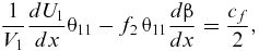 $$\begin{equation}
\frac{1}{{{V_1}}}\frac{{d{U_1}}}{{dx}}{\theta _{11}} - {f_2}\,{\theta _{11}}\frac{{d\beta }}{{dx}} = \frac{{{c_f}}}{2},
\end{equation}$$
$$\begin{equation}
\frac{1}{{{V_1}}}\frac{{d{U_1}}}{{dx}}{\theta _{11}} - {f_2}\,{\theta _{11}}\frac{{d\beta }}{{dx}} = \frac{{{c_f}}}{2},
\end{equation}$$
 $$\begin{equation}
2{f_4}{\left( {{\theta _{11}}\frac{{d\beta }}{{dx}}} \right)^2} + \left( {\frac{{{c_f}}}{2} - \frac{{3{f_1}}}{{{V_1}}}\frac{{d{U_1}}}{{dx}}{\theta _{11}}} \right)\left( {{\theta _{11}}\frac{{d\beta }}{{dx}}} \right) + \left( {H + 1} \right)\;{\left( {\frac{1}{{{V_1}}}\frac{{d{U_1}}}{{dx}}{\theta _{11}}} \right)^2} = 0,
\end{equation}$$
$$\begin{equation}
2{f_4}{\left( {{\theta _{11}}\frac{{d\beta }}{{dx}}} \right)^2} + \left( {\frac{{{c_f}}}{2} - \frac{{3{f_1}}}{{{V_1}}}\frac{{d{U_1}}}{{dx}}{\theta _{11}}} \right)\left( {{\theta _{11}}\frac{{d\beta }}{{dx}}} \right) + \left( {H + 1} \right)\;{\left( {\frac{1}{{{V_1}}}\frac{{d{U_1}}}{{dx}}{\theta _{11}}} \right)^2} = 0,
\end{equation}$$
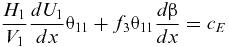 $$\begin{equation}
\frac{{{H_1}}}{{{V_1}}}\frac{{d{U_1}}}{{dx}}{\theta _{11}} + {f_3}{\theta _{11}}\frac{{d\beta }}{{dx}} = {c_E}
\end{equation}$$
$$\begin{equation}
\frac{{{H_1}}}{{{V_1}}}\frac{{d{U_1}}}{{dx}}{\theta _{11}} + {f_3}{\theta _{11}}\frac{{d\beta }}{{dx}} = {c_E}
\end{equation}$$
Note that U 1 and V 1 (see appendix) are re-introduced in the above equations, rather than ψ, for clarity. These equations can be solved iteratively but straightforwardly to obtain the momentum thickness and rate-of-change of limiting streamline angle at the AL (the rate of change of U 1 is a boundary condition given by the inviscid flowfield). The AL solution provides the initial values for Equation (7) which, in principle, can be solved at any point downstream of the AL, given the finite rate of change of both U 1 (and therefore ψ) and β at the AL. It turns out that, depending upon the resolution of the computational domain very near the AL, Equation (7) is ill-posed until a short distance downstream of the AL – the experience of the authors has been that the system of integral equations cannot be robustly tackled with a Runge-Kutta scheme until the angle ψ has decreased to about 80°. Similar difficulties were reported by Thompson and McDonald(Reference Thompson and McDonald18) and later by Smith(Reference Smith17), who adopted a numerical fix similar to the one employed by Callisto and described below. The issue may not have been encountered more widely because the problem region accounts for less than 1% of the chord length and would not impact upon less finely resolved computations. However, standards of resolution for the analysis of leading-edge flows have tightened in recent years, owing to the need to resolve the development of crossflow instability on laminar leading edges: adoption of the same numerical domain for the analysis of swept wings with turbulent AL invariably throws up this numerical feature.
2.4 Leading Edge Approximation
On the basis that the rates of change of both ψ and β are small for some distance downstream of the AL, a numerical fix was devised, involving a simple extrapolation of the AL similarity solution, used by Cumpsty and Head(Reference Cumpsty and Head16) and Smith(Reference Smith17) over the region where the integral equations were ill-posed, as defined by the criterion ψ > 80°. Such a sacrifice of accuracy for robustness was justified on the basis of the very short region concerned and the strongly favourable pressure gradient over this region, leading to the belief that the downstream development of the boundary layer integral quantities would not be significantly affected, hence providing acceptable accuracy for the calculation of the profile drag. This assumption appears to have been justified, but a fuller discussion is left until later in the paper, along with the demonstration of the effect of this numerical fix on the solution of the boundary layer equations. At this point we simply observe that there were no experimental data available to validate this approximation – hence the experimental study reported below.
3.0 EXPERIMENTAL INVESTIGATION
3.1 Experimental set-up and procedures
The experimental AL was generated on NACA0050 aerofoil profile, at zero angle of incidence, swept back by 60°. The model was made of wood with a normal-to-LE chord length of 466mm and a LE radius of curvature of 114mm. It was mounted between the floor and ceiling of the test section of the T2 wind tunnel in the Handley Page Laboratory at City, University of London, as shown in Fig. 4.

Figure 4. Schematic of the swept-wing model mounted in the T2 wind tunnel.
The T2 tunnel has a speed range of 4–55m/s. The test section measures 1120mm wide by 800mm high by 1.2m long: the model extended into the tunnel diffuser by 150mm. The blockage ratio introduced by such a large model is mitigated to an extent by the high sweep angle. Because the present investigation is focused on the flow very near the swept leading edge, the necessary numerical adjustments to the accompanying calculations can be achieved by an ‘effective sweep’ correction which infers the true magnitude of the velocity component parallel to the attachment line based upon the measured value of the pressure coefficient at the attachment line. The reader is referred to Ref. Reference Gowree, Atkin and Grupppetta9 for a comparison of the chordwise pressure distributions obtained from parallel rows of pressure taps around the model near the root (bottom), mid-span and tip sections. These pressure distributions and subsequent flow visualisations suggest that the flow separated at about 80% chord over most of the span of the model.
A surface-mounted boundary layer traverse probe with micro-displacement capability was employed to capture the velocity profile, with a resolution of 2.5μm per step achievable within an accuracy of ±0.09μm. This traverse, and the optical system used to calibrate probe displacement from the surface, is described in detail by Gowree et al(Reference Gowree, Atkin and Grupppetta9) for measurements on the attachment line (almost exactly on the model centreline). The right-hand image in Fig. 5 shows the additions made to the traverse, still fixed to the centreline line of the model, to allow the hot-wire probe to survey the flow away from the attachment line. The left-hand image illustrates how the axis of the optical alignment system was inclined to enable the same technique as described in Ref. Reference Gowree, Atkin and Grupppetta9 to be used for determining distance between probe and model surface.

Figure 5. Arrangement used to apply the techniques used by Gowree et al(Reference Gowree, Atkin and Grupppetta9) to probe the flow away from the leading edge of the model.
A single normal (SN) hot-wire probe, Dantec 55P15, was used to capture the single velocity component at the AL and a Single Yawed (SY) probe, 55P12, for the measurement of the two in-plane velocity components downstream of the AL. The Constant Temperature Anemometry (CTA) technique was used and the hot-wire probes were connected to the DISA-55M10 CTA Standard Bridge (M-Unit) module. The M-Unit was in turn interfaced with a National Instruments (NI)-DAQ card with built-in A/D converter and installed in a PC for data acquisition using NI LabVIEW. The hot-wire output signal, sampled for 10 seconds at 10 kHz, was pre-filtered through a low-pass filter rated at 4.8kHz prior to recording. King's law was applied for the reduction of hot-wire output voltage. The calibration of the SN probe and measurement of a single velocity component at the AL was straightforward, but more challenging for the SY probe used to measure the two velocity components immediately downstream of the AL. In this case, Bradshaw's method described in Ref. Reference Gowree19 was employed and a yaw calibration was required due to the directional sensitivity of the SY probe. The estimated error for the hot-wire measurements was less than 5%(Reference Gowree19) but the excellent agreement between the measured velocity profiles along a laminar attachment line and the theoretical solution for swept Hiemenz flow (Fig 17 of Ref. Reference Gowree, Atkin and Grupppetta9) suggests that the actual error, including probe interference, was marginal.
Preston's(Reference Preston20) technique was employed for the measurement of local surface shear stress. At the AL, the flow resolves into a single spanwise velocity component, similar to the streamwise flow along a flat plate, thus the method was expected to yield reasonable accuracy. This technique has thus far been restricted to 2D flows where the skin friction acts in the same direction as the velocity component; however, for the flow downstream of the AL, an attempt was made to extend this technique to the 3D boundary layer under the highly curved streamline at the LE of a swept wing. The surface shear stress measurement was made by aligning the pitot tube in the direction of the local external streamline, obtained from the velocity components measured using the CTA technique at the edge of the boundary layer. The angle between the external and the surface streamlines was small (approximately ±5° as discussed in Section 4.2), and therefore this approach was felt to add negligible additional error: the uncertainty analysis conducted by Gowree(Reference Gowree19) yielded the same confidence level as for the 2D case of purely spanwise flow along the attachment line.
4.0 EXPERIMENTAL RESULTS
4.1 Streamwise velocity profiles
Due to contamination by the turbulent boundary layer on the floor of the wind tunnel, the flow along the AL was found to be intermittently turbulent for R θ > 100. This threshold is in agreement with the results of Pfenninger(Reference Pfenninger21) and Gaster(Reference Gaster22). The turbulent mean velocity profiles were captured at various AL Reynolds numbers and, using the surface shear stress measurements, these profiles were represented in wall units, Fig. 6. For the fully turbulent velocity profiles, some measurements were acquired in the laminar sub-layer despite a boundary layer thickness of the order of 3mm, owing to the digital optical system(Reference Gowree, Atkin and Grupppetta9) which enabled the hot-wire probe to be positioned accurately very close to the wall. Figure 6 shows that the logarithmic region of the velocity profiles deviates from the universal log-law used by Cumpsty and Head(Reference Cumpsty and Head16), although significant scatter was observed in the latter's experimental results. Spalart(Reference Spalart23) suggested, on the basis of DNS analysis, that on a flat plate, for R θ < 620, the log-law was best defined using the von Kármán constant, k = 0.41. In the present work on the attachment line, the best fit to the experimental data was obtained using k = 0.39.

Figure 6. The turbulent velocity profile at the AL.
The mean streamwise velocity profiles captured just downstream of the AL are presented in Fig. 7 for an AL Reynolds number R θ = 590. The good agreement between the port and starboard side measurements demonstrates that the AL was coincident with the leading edge of the model.

Figure 7. Streamwise velocity profiles at the LE for an AL R θ = 590.
Using the surface shear stress measurements the velocity profiles were represented in wall units, as shown in Fig. 8. The inner region of these velocity profiles matches the ‘universal log-law’ with reasonable agreement, but the measurements in the viscous sub-layer vary irregularly with chordwise position. However, the agreement with the universal log-law suggests that the profiles were captured with reasonable accuracy outside the sub-layer and can be useful for further analysis.

Figure 8. Streamwise velocity profiles in wall units, downstream of the AL at R θ = 590.
4.2 Crossflow velocity profiles
Figure 9 shows the crossflow profiles (velocity perpendicular to the external streamline, as opposed to the spanwise direction) at different chordwise positions downstream of the AL. Good agreement can be observed between the port and starboard measurements except at x/c = 0.03. This is probably due to the limitation in the yaw sensitivity of the SY probe which was, in anticipation, restricted to ±70° during the yaw calibration. More detail of the crossflow was revealed when the profiles were plotted on the triangular hodograph model proposed by Johnston(Reference Johnston24), as shown in Fig. 10, where the normalised crossflow velocity can be represented as a function of streamwise velocity. From Fig. 10 it is easier to detect the development of the ‘S-type’ or ‘crossover’ crossflow profiles which are present for x/c > 0.0025. Normally, the crossover point occurs very close to the wall and shifts upwards further downstream, as observed in Fig. 10. Due to limited resolution in the near wall measurements, it is difficult to capture the chordwise location where the crossover first develops. The main issue with the triangular representation is the difficulty in applying a linear fit to the profiles, especially around the maxima of the crossflow velocity.

Figure 9. Crossflow velocity profiles downstream of the AL at R θ = 590.

Figure 10. Triangular representation of crossflow profiles using Johnston's model.
According to Johnston, the angle between the limiting and the external streamline, β, can be approximated as the gradient of the line of best fit connecting the origin and the apex of the triangle defined by the stationary points (maxima or minima) of the velocity profiles, which is assumed to be the region where the surface shear stress is dominant. Using this approach, on the port side of the model at x/c = 0.0025, the angle between the limiting and external streamline, β, is –3.1°. The same method can be applied to the crossover profile but, due to insufficient data in the near wall region for the measurement between 0.01 ≤ x/c ≤ 0.02, it was not possible to determine β until x/c = 0.03, where the apex of the triangle could be resolved. At this position, linear extrapolation of the velocity components suggests a limiting value of β = 18°. It appears unlikely from Fig. 10 that β attains large negative values before the appearance of the crossover in the crossflow profiles: therefore, it seems fair to assume that, within the current experimental domain, the limiting streamline angle ranged between –3° < β < 18° and, nearer the attachment line, x/c ≤ 0.01, it appears that |β| < 3°. Given that one might have expected the near-wall flow to respond more rapidly than the inviscid flow to the very strong pressure gradient acting nearly perpendicular to the direction of flow in this region, the limiting streamline angles are perhaps surprisingly small in value.
4.3 Topology of the flow at the leading edge
The external inviscid streamline can be resolved in terms of the chordwise and spanwise velocity components measured at the edge of the boundary layer using the SY probe. The variation in the streamline angle, ψ, relative to the normal-to-LE direction is plotted in Fig. 11. At x/c = 0.0, ψ ≈ 90° as the flow along the AL is purely spanwise and at x/c > 0.03 the external streamline is nearly aligned with the free stream.

Figure 11. The orientation of the external streamline with respect to the chord normal to the LE at an AL of Rθ = 590.
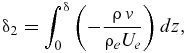
In addition to the streamwise momentum thickness defined in Equation (4) above, the following streamwise and crossflow boundary layer integral quantities were derived from the experimentally measured streamwise and crossflow velocity profiles (under incompressible conditions, ρ = ρe ) which were captured within an accuracy of ±5%; the development of these length scales in the vicinity of the AL is presented in Fig. 12.
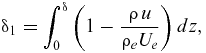 $$\begin{equation}
{\delta _1} = \int_0^\delta {\left( {1 - \frac{{\rho \,u}}{{{\rho _e}{U_e}}}} \right)dz} ,\\
\end{equation}$$
$$\begin{equation}
{\delta _1} = \int_0^\delta {\left( {1 - \frac{{\rho \,u}}{{{\rho _e}{U_e}}}} \right)dz} ,\\
\end{equation}$$
 $$\begin{equation}
{\delta _2} = \int_0^\delta {\left( { - \frac{{\rho \,\hbox{v}}}{{{\rho _e}{U_e}}}} \right)dz} ,\\
\end{equation}$$
$$\begin{equation}
{\delta _2} = \int_0^\delta {\left( { - \frac{{\rho \,\hbox{v}}}{{{\rho _e}{U_e}}}} \right)dz} ,\\
\end{equation}$$
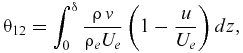 $$\begin{equation}
{\theta _{12}} = \int_0^\delta {\frac{{\rho \,\hbox{v}}}{{{\rho _e}{U_e}}}\left( {1 - \frac{u}{{{U_e}}}} \right)dz} ,\\
\end{equation}$$
$$\begin{equation}
{\theta _{12}} = \int_0^\delta {\frac{{\rho \,\hbox{v}}}{{{\rho _e}{U_e}}}\left( {1 - \frac{u}{{{U_e}}}} \right)dz} ,\\
\end{equation}$$
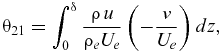 $$\begin{equation}
{\theta _{21}} = \int_0^\delta {\frac{{\rho \,u}}{{{\rho _e}{U_e}}}\left( { - \frac{\hbox{v}}{{{U_e}}}} \right)dz} ,\\
\end{equation}$$
$$\begin{equation}
{\theta _{21}} = \int_0^\delta {\frac{{\rho \,u}}{{{\rho _e}{U_e}}}\left( { - \frac{\hbox{v}}{{{U_e}}}} \right)dz} ,\\
\end{equation}$$
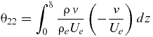 $$\begin{equation}
{\theta _{22}} = \int_0^\delta {\frac{{\rho \,\hbox{v}}}{{{\rho _e}{U_e}}}\left( { - \frac{\hbox{v}}{{{U_e}}}} \right)dz}
\end{equation}$$
$$\begin{equation}
{\theta _{22}} = \int_0^\delta {\frac{{\rho \,\hbox{v}}}{{{\rho _e}{U_e}}}\left( { - \frac{\hbox{v}}{{{U_e}}}} \right)dz}
\end{equation}$$

Figure 12. The port side streamwise and crossflow integral quantities in the vicinity of the AL at R θ = 590.
The streamwise momentum thickness, θ11, increases by approximately 15% immediately downstream of the AL, and so does the streamwise displacement thickness, δ1. A slightly non-monotonic trend can be observed in the development of θ11 and δ1, which was initially thought to be due to experimental uncertainty. But error analysis suggested that these differences were significantly larger than ±5% and therefore could potentially be due to an unexpected physical behaviour of the turbulent boundary layer. The crossflow momentum thicknesses θ12 and θ22 are almost negligible at the AL (as expected from the very small magnitudes of the crossflow velocity) and do not vary significantly downstream. However, θ21 grows to about one-third of the value of θ11 and δ2 to roughly one-eighth of the value of δ1. This growth in the integral quantities is significant and is not captured by the LE approximation in Callisto, prompting the numerical modelling to be revisited.
5.0 MODIFICATIONS TO THE GOVERNING EQUATIONS IN CALLISTO
5.1 Modification to leading edge model
As discussed previously, in Callisto a numerical approximation to the governing equations is imposed near the AL, specifically while ψ > 80°. For the current experiment this zone ends somewhere in the region 0.005 < x/c < 0.01, as shown in Fig. 11. As discussed at the end of Section 4.2, in this region the limiting streamline angle appears to be small in magnitude, |β| < 3°. This experimental observation suggests that the governing equations might remain ill-posed immediately downstream of the AL not simply because cosψ ≈ 0, but because tanβ is also small in the same region: the slow development of cosψ and tanβ means that the system of Equations (7) remains dominated by just two terms out of nine close to the attachment line (see discussion in Section 2.3). This results in numerical error and poor robustness when marching the boundary layer equations using a Runge-Kutta scheme. A new, more subtle numerical approximation to the governing equations was therefore developed: to extend the assumption – by Cumpsty and Head(Reference Cumpsty and Head16) and Smith(Reference Cumpsty and Head16) – of constant, finite ∂β/∂x at the AL to the flow immediately downstream. This allows the normal momentum equation to be de-coupled, allowing the remaining two equations to be solved as a coupled system, as shown below:
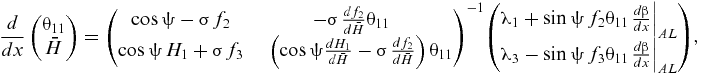 $$\begin{eqnarray}
\frac{d}{{dx}}\left( {\begin{array}{@{}*{1}{c}@{}} {{\theta _{11}}}\\ {\bar{H}} \end{array}} \right) = {\left( {\begin{array}{@{}*{2}{c}@{}} {\cos \psi - \sigma \,{f_2}}&{ - \sigma \,\frac{{d{f_2}}}{{d\bar{H}}}{\theta _{11}}}\\ {\cos \psi \,{H_1} + \sigma \,{f_3}}&\quad{\left( {\cos \psi \frac{{d{H_1}}}{{d\bar{H}}} - \sigma \,\frac{{d{f_2}}}{{d\bar{H}}}} \right){\theta _{11}}} \end{array}} \right)^{ - 1}}\!\left( {\begin{array}{@{}*{1}{c}@{}} {{\lambda _1} + \sin \psi \,{f_2}{\theta _{11}}{{\left. {\frac{{d\beta }}{{dx}}} \right|}_{AL}}}\\ {{\lambda _3} - \sin \psi \,{f_3}{\theta _{11}}{{\left. {\frac{{d\beta }}{{dx}}} \right|}_{AL}}} \end{array}} \right)\!,\nonumber\\
\end{eqnarray}$$
$$\begin{eqnarray}
\frac{d}{{dx}}\left( {\begin{array}{@{}*{1}{c}@{}} {{\theta _{11}}}\\ {\bar{H}} \end{array}} \right) = {\left( {\begin{array}{@{}*{2}{c}@{}} {\cos \psi - \sigma \,{f_2}}&{ - \sigma \,\frac{{d{f_2}}}{{d\bar{H}}}{\theta _{11}}}\\ {\cos \psi \,{H_1} + \sigma \,{f_3}}&\quad{\left( {\cos \psi \frac{{d{H_1}}}{{d\bar{H}}} - \sigma \,\frac{{d{f_2}}}{{d\bar{H}}}} \right){\theta _{11}}} \end{array}} \right)^{ - 1}}\!\left( {\begin{array}{@{}*{1}{c}@{}} {{\lambda _1} + \sin \psi \,{f_2}{\theta _{11}}{{\left. {\frac{{d\beta }}{{dx}}} \right|}_{AL}}}\\ {{\lambda _3} - \sin \psi \,{f_3}{\theta _{11}}{{\left. {\frac{{d\beta }}{{dx}}} \right|}_{AL}}} \end{array}} \right)\!,\nonumber\\
\end{eqnarray}$$
 $$\begin{equation}
\frac{{d\beta }}{{dx}} = {\left. {\frac{{d\beta }}{{dx}}} \right|_{AL}}
\end{equation}$$
$$\begin{equation}
\frac{{d\beta }}{{dx}} = {\left. {\frac{{d\beta }}{{dx}}} \right|_{AL}}
\end{equation}$$
The experimental results actually show that ∂β/∂x does vary downstream of the attachment line, so Equation (20) can be thought of as the first term of an expansion for ∂β/∂x. In this respect we are primarily looking for a more robust numerical treatment rather than for a model of the highest accuracy. Moreover no attempt has been made (nor could be, given the sparseness of the crossflow profile data obtained) to improve the Mager(Reference Preston25) crossflow profile modelling (see Appendix) which – as is well-known – cannot cater for the type of crossover profiles seen in the experimental results.
The revised solution process is then as follows: the first task is to solve the simultaneous system described by Equations (10) through (12) for θ 11, H (and therefore H ) and ∂β / ∂x at the AL; immediately downstream of the AL, Equations (18) and (19) are used to march the solution until tan β recovers to a threshold value, whereupon the full 3D system of Equations (7) can be restored. This threshold value is determined by numerical robustness and is so small that the switch from Equation (18) to the full 3D form – Equation (7) – is hardly detectable in the results.
5.2 Results obtained using the modification governing equations
The development of the streamwise momentum thickness obtained from the computation with the improved LE modelling (new) can be compared with those from the previous version of Callisto (old) in Fig. 13, where s/c represents the normalised coordinate along the surface of wing profile in the direction normal to the leading edge. Computations with the modified code were conducted for both the geometrical sweep condition, 60°, and the effective sweep, which was calculated to be approximately 62° using the experimental static pressure at x/c = 0 (see Section 5.4.1 in Ref. Reference Gowree19 for more details). These results are presented in Fig. 13 which shows a slight asymmetry in the computed results near the leading edge: Callisto-VGK captures the significant trailing edge separation present over the aft 10% chord of the model, but the resulting solution is mildly oscillatory (residual convergence to 10–4 rather than the usual 10–6 employed for aerofoil analyses) and any given ‘snapshot’ of the solution will feature some small circulation around the model, which results in the asymmetry visible in the figure.

Figure 13. Comparison of θ values captured experimentally against those computed using the original and the modified versions of Callisto.
In Fig. 13, looking at the prediction from the original version of Callisto, θ11 remains constant immediately downstream of the AL – due to the extrapolation of the attachment line solution – and then starts to increase again once a solution of the full governing equations is obtained, for ψ < 80°. In the modified version, the reduced set of governing equations can be solved immediately downstream of the AL: a comparison between the computed results and experimental results in Fig. 13 shows a significant improvement, as the momentum thickness is now predicted to be within ±5% of the experimental results. The non-monotonic behaviour in the experimental momentum thickness is also now replicated by the numerical results, providing confidence in the experimental observation.
Figure 14 shows the computed development of the limiting streamline angle and the transformed shape factor before and after the modifications to Callisto; these results all include the effective sweep correction. Callisto employs a continuous coordinate system sʹ (the developed surface distance around the model, normal to the leading edge) so that the sign convention for β differs on one side of the model, compared to the experiment. The method predicts a maximum value of β of around 13° at sʹ ≈ 0.13, (corresponding to x/c ≈ 0.03) as compared with the 18° estimated at this location from the experimental velocity profiles. This discrepancy is attributed to the relative simplicity of the Mager model used to capture the crossflow (as discussed in Section 5.1). The new treatment of the governing equations has a relatively small impact on the development of β: a slight discontinuity in ∂β/∂x, where the method switches from a constant AL value to direct calculation of the derivative using the marching scheme in equation (7), is visible in both cases. This suggests that the third derivative ∂3β/∂x3 , which is not resolved by either approach, is of significant magnitude of at the AL. Interestingly the relative magnitudes of β predicted by the old and new schemes are then reversed by the marching scheme, before converging much further downstream (off the ends of the plot). The shape factor H is also seen to be fixed at a constant AL value by the old scheme, whereas the new scheme again allows a more rapid return to the trends predicted by the marching scheme. Overall the figure illustrates the advantage of the new approach in allowing Callisto to switch to the full system of equations at an earlier point in the analysis, owing to the more precise diagnosis of the robustness problems in the governing equations; however, there is little evidence that the flow development a long way downstream of the AL would be sensitive to the change in leading-edge modelling – at least for this particular case.

Figure 14.
β and
 $\bar{H}$
values computed using the original and the modified versions of Callisto.
$\bar{H}$
values computed using the original and the modified versions of Callisto.
6.0 DISCUSSION
Figure 6 shows that, for Rθ ≥ 315, the logarithmic regions of the velocity profiles collapse onto a single (modified) log-law. This finding is in agreement with Preston's(Reference Preston25) criterion for minimum Reynolds number for the existence of a fully turbulent boundary layer on a flat plate for Rθ ≈ 320. Similar behaviour was also reported during the DNS study of Spalart(Reference Spalart26), where the inner layer of the velocity profiles tended towards the universal log-law at Rθ > 300. Based on this result a new regime where the AL is intermittent can be defined for 100 < Rθ < 315. It is our belief that the AL has been previously misinterpreted to be fully turbulent in this regime, which is misleading in the context of flow control applications on swept wings. In addition, on the mid-span and outboard section of the wings of short-haul airliners, and the outboard section of long-haul airliners, Rθ < 300; therefore, numerical analysis which assumes fully turbulent flow right from the AL is likely to be incorrect.
The marked growth in the boundary layer momentum thickness observed experimentally immediately downstream of the AL underlines the need for improved modelling in Callisto. The modification to the governing equations in the vicinity of the AL can be considered satisfactory due to the much-improved agreement between the calculated and the experimental results.
Despite the significant change in the AL modelling, the profile drag prediction was not significantly affected: the predicted momentum thickness in the far wake was almost the same from both the old and the new versions of Callisto. The revised computational results in Fig. 13 show a rapid growth in momentum thickness downstream of the AL followed by an equally rapid decay, presumably due to the interplay between streamline curvature and favourable pressure gradient at the LE. From the mean flow measurements it is difficult to understand and describe the physical mechanism responsible for the non-monotonic growth in θ 11 in the vicinity of the AL, but as a similar trend was predicted by Callisto, a simple diagnosis was conducted by analysing the individual terms of the streamwise momentum integral equation. The local maximum in θ 11 appears when the magnitude of the favourable pressure gradient exceeds the skin friction immediately downstream of the AL, hence reversing the growth in θ 11. The minimum is associated with the relaxation of the favourable pressure gradient to a point where the skin friction once again dominates, so that θ 11 grows again. This interesting trend reversal is partly a consequence of the streamline analogy implicit in the treatment of turbulence by Head's entrainment model, but it is clearly reproduced to an extent by the flowfield measurements. From the experimental perspective, the question is whether or not these streamwise-resolved integral properties provide the most insight into the physics of the flowfield at the AL.
By x/c = 0.25, θ 11 estimated by the modified Callisto is very similar to that obtained from the original version, any residual differences being smaller than the effect of correcting for effective sweep. Similar behaviour has also been observed during the analysis of the leading edge flow over a transonic wing at cruise condition. Based on these observations, the overall profile drag predictions obtained from earlier versions of Callisto can still be considered robust.
The formation of crossover crossflow profiles in laminar boundary layers is usually associated with a change in sign of the chordwise pressure gradient (which, from the perspective of the streamlines very close to the AL, acts in the crossflow direction) accompanied by an inflection point in the external streamline; however, the monotonic trend in streamline direction seen in Fig. 11 rules out that explanation for the crossover in the turbulent crossflow velocity profiles observed in the present experiment for x/c > 0.0025. Following analysis of the transverse momentum equation in curvilinear coordinates, Gowree(Reference Gowree19) suggested that, along a fully turbulent, highly curved streamline, this effect might occur due to the rapid growth in transverse Reynolds stresses, compared to the gradually decaying crossflow component of pressure gradient, resulting in a change of sign of the resultant transverse force acting on the boundary layer flow and the consequent appearance of crossover profiles.
7.0 CONCLUSIONS
Measurements at the leading edge of a swept wing model have helped to shed some light on the development of the turbulent flow along a swept AL and have yielded a threshold Reynolds number for a fully developed turbulent AL that is consistent with Preston's criterion for the turbulent flow on a flat plate.
Based on the observed small values of limiting streamline angle, β, near the AL, a new approach to solving the 3D momentum integral equations near the AL has been implemented in the Airbus Callisto method, solving a 50-year-old numerical problem. The results from the revised method show good agreement with the experimental measurements, correctly capturing the observed non-monotonic behaviour of θ 11 in this region. Although significant improvement in computing power has allowed the modelling of such flows using DNS and LES that has enriched our understanding of the mechanics of fluids, there is still value in developing low-order integral boundary layer methods to be able to capture relevant physical phenomena such as those explored in this paper, as the benefits of flow control and similar technologies will need to be captured as early as possible in the design process.
The present experimental results can also be of use for the validation of higher-order turbulence models which are aimed at capturing the effect of lateral strain from highly diverging or converging streamlines.
APPENDIX
GOVERNING EQUATIONS
We start with the work of Ashill and Smith(Reference Ashill and Smith12) who derived a system of three integral equations for momentum, resolved parallel and normal to the inviscid flow streamline, and entrainment expressed in the conical-surface (x,y) coordinate system illustrated in Fig. 2:
 $$\begin{equation}
\left( {\begin{array}{@{}*{3}{c}@{}} {{A_{11}}}&{{A_{12}}}&{{A_{13}}}\\ {{A_{21}}}&\ {{A_{22}}}&\ {{A_{23}}}\\ {{A_{31}}}&{{A_{32}}}&{{A_{33}}} \end{array}} \right)\frac{d}{{dx}}\left( {\begin{array}{@{}*{1}{c}@{}} {{\theta _{11}}}\\ {\tan \beta }\\ {{H_1}{\theta _{11}}} \end{array}} \right) = \;\left( {\begin{array}{@{}*{1}{c}@{}} {{\lambda _1}}\\ {{\lambda _2}}\\ {{\lambda _3}} \end{array}} \right)
\end{equation}$$
$$\begin{equation}
\left( {\begin{array}{@{}*{3}{c}@{}} {{A_{11}}}&{{A_{12}}}&{{A_{13}}}\\ {{A_{21}}}&\ {{A_{22}}}&\ {{A_{23}}}\\ {{A_{31}}}&{{A_{32}}}&{{A_{33}}} \end{array}} \right)\frac{d}{{dx}}\left( {\begin{array}{@{}*{1}{c}@{}} {{\theta _{11}}}\\ {\tan \beta }\\ {{H_1}{\theta _{11}}} \end{array}} \right) = \;\left( {\begin{array}{@{}*{1}{c}@{}} {{\lambda _1}}\\ {{\lambda _2}}\\ {{\lambda _3}} \end{array}} \right)
\end{equation}$$
The various coefficients in this equation are defined as follows:
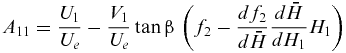 $$\begin{equation}
{A_{11}} = \frac{{{U_1}}}{{{U_e}}} - \frac{{{V_1}}}{{{U_e}}}\tan \beta \,\left( {{f_2} - \frac{{d{f_2}}}{{d\bar{H}}}\frac{{d\bar{H}}}{{d{H_1}}}{H_1}} \right)
\end{equation}$$
$$\begin{equation}
{A_{11}} = \frac{{{U_1}}}{{{U_e}}} - \frac{{{V_1}}}{{{U_e}}}\tan \beta \,\left( {{f_2} - \frac{{d{f_2}}}{{d\bar{H}}}\frac{{d\bar{H}}}{{d{H_1}}}{H_1}} \right)
\end{equation}$$
The notation above differs slightly to that used by Ashill and Smith(Reference Ashill and Smith12) in that the symbols U 1 and V 1 are used for the normal-to-generator and parallel-to-generator components of the inviscid velocity field outside the boundary layer, rather than the symbols Uχ and VR respectively. Moreover V 1 is positive towards the wing tip whereas VR is positive towards the wing root.
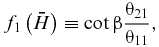
The factor f 2 above captures the relationship between the crossflow momentum thickness θ 12, Equation (15), and the streamwise momentum thickness θ 11, Equation (4), as follows
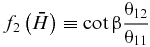 $$\begin{equation}
{f_2}\left( {\bar{H}} \right) \equiv \cot \beta \frac{{{\theta _{12}}}}{{{\theta _{11}}}}
\end{equation}$$
$$\begin{equation}
{f_2}\left( {\bar{H}} \right) \equiv \cot \beta \frac{{{\theta _{12}}}}{{{\theta _{11}}}}
\end{equation}$$
This and the other closure relationships
 ${f_n}( {\bar{H}} )$
are determined by assuming the form of the velocity profiles within the boundary layer, as is typical for integral methods: it simplifies the analysis considerably to assume that these profiles are a function only of transformed shape factor
H
, Equation (6). The closures popular with the RAE lag-entrainment codes, of which Callisto is one family member, are based on the crossflow velocity profiles proposed by Mager(Reference Mager27) and are detailed in Smith(Reference Smith17). How representative these profiles are of 3D boundary layers in adverse pressure gradients has been the subject of much debate, but is beyond the scope of this paper. Suffice to say that expressions of the form of Equation (A.3) are key to the closure of the system of three-dimensional, integral equations. The transformed shape factor
H
is usually related to the classical shape factor for compressible boundary layer flow by the following expression(Reference Green13).
${f_n}( {\bar{H}} )$
are determined by assuming the form of the velocity profiles within the boundary layer, as is typical for integral methods: it simplifies the analysis considerably to assume that these profiles are a function only of transformed shape factor
H
, Equation (6). The closures popular with the RAE lag-entrainment codes, of which Callisto is one family member, are based on the crossflow velocity profiles proposed by Mager(Reference Mager27) and are detailed in Smith(Reference Smith17). How representative these profiles are of 3D boundary layers in adverse pressure gradients has been the subject of much debate, but is beyond the scope of this paper. Suffice to say that expressions of the form of Equation (A.3) are key to the closure of the system of three-dimensional, integral equations. The transformed shape factor
H
is usually related to the classical shape factor for compressible boundary layer flow by the following expression(Reference Green13).
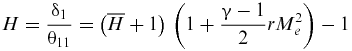 $$\begin{equation}
H = \frac{{{\delta _1}}}{{{\theta _{11}}}} = \left( {\overline H + 1} \right)\,\left( {1 + \frac{{\gamma - 1}}{2}rM_e^2} \right) - 1
\end{equation}$$
$$\begin{equation}
H = \frac{{{\delta _1}}}{{{\theta _{11}}}} = \left( {\overline H + 1} \right)\,\left( {1 + \frac{{\gamma - 1}}{2}rM_e^2} \right) - 1
\end{equation}$$
where δ 1 is defined in Equation (13) and where r is the recovery factor. Also appearing in Equation (A.2) above is the entrainment shape factor H 1 defined as
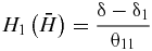 $$\begin{equation}
{H_1}\left( {\bar{H}} \right) = \frac{{\delta - {\delta _1}}}{{{\theta _{11}}}}
\end{equation}$$
$$\begin{equation}
{H_1}\left( {\bar{H}} \right) = \frac{{\delta - {\delta _1}}}{{{\theta _{11}}}}
\end{equation}$$
As with the closure relationships
 ${f_n}( {\bar{H}} )$
, the functional dependence
${f_n}( {\bar{H}} )$
, the functional dependence
 ${H_1}( {\bar{H}} )$
has been the subject of much discussion(Reference Lock and Williams4). Suffice to say that the observed singularity in the boundary layer equations at separation is captured by entrainment-based integral methods only if the derivative
${H_1}( {\bar{H}} )$
has been the subject of much discussion(Reference Lock and Williams4). Suffice to say that the observed singularity in the boundary layer equations at separation is captured by entrainment-based integral methods only if the derivative
 ${{d{H_1}}/ {d\bar{H}}}$
changes sign at separation. As with the rank of the boundary layer equations, the problem of separating flows is not within the scope of this paper.
${{d{H_1}}/ {d\bar{H}}}$
changes sign at separation. As with the rank of the boundary layer equations, the problem of separating flows is not within the scope of this paper.
The remaining coefficients of the streamwise momentum equation are as follows:
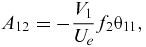 $$\begin{equation}
{A_{12}} = - \frac{{{V_1}}}{{{U_e}}}{f_2}{\theta _{11}},
\end{equation}$$
$$\begin{equation}
{A_{12}} = - \frac{{{V_1}}}{{{U_e}}}{f_2}{\theta _{11}},
\end{equation}$$
 $$\begin{equation}
{A_{13}} = - \frac{{{V_1}}}{{{U_e}}}\tan \beta \,\frac{{d{f_2}}}{{d\bar{H}}}\frac{{d\bar{H}}}{{d{H_1}}},
\end{equation}$$
$$\begin{equation}
{A_{13}} = - \frac{{{V_1}}}{{{U_e}}}\tan \beta \,\frac{{d{f_2}}}{{d\bar{H}}}\frac{{d\bar{H}}}{{d{H_1}}},
\end{equation}$$
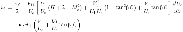 $$\begin{eqnarray}
\, {\lambda _1} &=&\frac{{{c_f}}}{2} - \displaystyle\frac{{{\theta _{11}}}}{{{U_e}}}\left[ {\displaystyle\frac{{{U_1}}}{{{U_e}}}\left( {H + 2 - M_e^2} \right) + \frac{{V_1^2}}{{{U_1}\,{U_e}}}\left( {1 - {{\tan }^2}\beta {f_4}} \right) + \frac{{{V_1}}}{{{U_e}}}\tan \beta {f_4}} \right]_{}^{}\displaystyle\frac{{d{U_e}}}{{dx}}\nonumber\\
&&+\, {\kappa _T}{\theta _{11}}\left( {\displaystyle\frac{{{V_1}}}{{{U_e}}} + \displaystyle\frac{{{U_1}}}{{{U_e}}}\tan \beta \,{f_2}} \right)
\end{eqnarray}$$
$$\begin{eqnarray}
\, {\lambda _1} &=&\frac{{{c_f}}}{2} - \displaystyle\frac{{{\theta _{11}}}}{{{U_e}}}\left[ {\displaystyle\frac{{{U_1}}}{{{U_e}}}\left( {H + 2 - M_e^2} \right) + \frac{{V_1^2}}{{{U_1}\,{U_e}}}\left( {1 - {{\tan }^2}\beta {f_4}} \right) + \frac{{{V_1}}}{{{U_e}}}\tan \beta {f_4}} \right]_{}^{}\displaystyle\frac{{d{U_e}}}{{dx}}\nonumber\\
&&+\, {\kappa _T}{\theta _{11}}\left( {\displaystyle\frac{{{V_1}}}{{{U_e}}} + \displaystyle\frac{{{U_1}}}{{{U_e}}}\tan \beta \,{f_2}} \right)
\end{eqnarray}$$
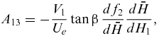
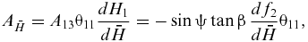
Again there is a slight difference in notation in Equation (A.8) compared to the equivalent equation quoted by Ashill and Smith(Reference Ashill and Smith12), the taper curvature term κT above appearing as ϕ/l, where ϕ is the angle AOC in Fig. 2 and l is the arc length AC. f4 in Equation (A.8) above is given by
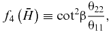 $$\begin{equation}
{f_4}\left( {\bar{H}} \right) \equiv {\cot ^2}\beta \frac{{{\theta _{22}}}}{{{\theta _{11}}}},
\end{equation}$$
$$\begin{equation}
{f_4}\left( {\bar{H}} \right) \equiv {\cot ^2}\beta \frac{{{\theta _{22}}}}{{{\theta _{11}}}},
\end{equation}$$
where θ 22 is defined in Equation (17)
The coefficients of the crossflow momentum integral equation are as follows:
 $$\begin{equation}
{A_{21}} = \tan \beta \left( {\frac{{{U_1}}}{{{U_e}}}{f_1} - \frac{{{V_1}}}{{{U_e}}}\tan \beta \,{f_4}} \right) - {H_1}\frac{{d\bar{H}}}{{d{H_1}}}\tan \beta \left( {\frac{{{U_1}}}{{{U_e}}}\frac{{d{f_1}}}{{d\bar{H}}} - \frac{{{V_1}}}{{{U_e}}}\tan \beta \frac{{d{f_4}}}{{d\bar{H}}}} \right),
\end{equation}$$
$$\begin{equation}
{A_{21}} = \tan \beta \left( {\frac{{{U_1}}}{{{U_e}}}{f_1} - \frac{{{V_1}}}{{{U_e}}}\tan \beta \,{f_4}} \right) - {H_1}\frac{{d\bar{H}}}{{d{H_1}}}\tan \beta \left( {\frac{{{U_1}}}{{{U_e}}}\frac{{d{f_1}}}{{d\bar{H}}} - \frac{{{V_1}}}{{{U_e}}}\tan \beta \frac{{d{f_4}}}{{d\bar{H}}}} \right),
\end{equation}$$
 $$\begin{equation}
{f_1}\left( {\bar{H}} \right) \equiv \cot \beta \frac{{{\theta _{21}}}}{{{\theta _{11}}}},
\end{equation}$$
$$\begin{equation}
{f_1}\left( {\bar{H}} \right) \equiv \cot \beta \frac{{{\theta _{21}}}}{{{\theta _{11}}}},
\end{equation}$$
where θ 21 is defined in Equation (16)
 $$\begin{equation}
{A_{22}} = \left( {\frac{{{U_1}}}{{{U_e}}}{f_1} - 2\frac{{{V_1}}}{{{U_e}}}\tan \beta \,{f_4}} \right)\,{\theta _{11}},\\
\end{equation}$$
$$\begin{equation}
{A_{22}} = \left( {\frac{{{U_1}}}{{{U_e}}}{f_1} - 2\frac{{{V_1}}}{{{U_e}}}\tan \beta \,{f_4}} \right)\,{\theta _{11}},\\
\end{equation}$$
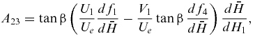 $$\begin{equation}
{A_{23}} = \tan \beta \left( {\frac{{{U_1}}}{{{U_e}}}\frac{{d{f_1}}}{{d\bar{H}}} - \frac{{{V_1}}}{{{U_e}}}\tan \beta \,\frac{{d{f_4}}}{{d\bar{H}}}} \right)\frac{{d\bar{H}}}{{d{H_1}}},\\
\end{equation}$$
$$\begin{equation}
{A_{23}} = \tan \beta \left( {\frac{{{U_1}}}{{{U_e}}}\frac{{d{f_1}}}{{d\bar{H}}} - \frac{{{V_1}}}{{{U_e}}}\tan \beta \,\frac{{d{f_4}}}{{d\bar{H}}}} \right)\frac{{d\bar{H}}}{{d{H_1}}},\\
\end{equation}$$
 $$\begin{eqnarray}
{\lambda _2} &=& \frac{{{c_f}}}{2}\tan \beta - {\left[ {\left( {2\frac{{{U_e}}}{{{U_1}}} - M_e^2\frac{{{U_1}}}{{{U_e}}}} \right)\tan \beta \,{f_1} - \frac{{{V_1}}}{{{U_e}}}\left( {1 + H + {{\tan }^2}\beta {f_4}\left\{ {1 - M_e^2} \right\}} \right)} \right]^{}}\frac{{{\theta _{11}}}}{{{U_e}}}\frac{{d{U_e}}}{{dx}}\nonumber\\
&&+\, {\kappa _T}{\theta _{11}}\tan \beta \left( {\frac{{{V_1}}}{{{U_e}}}{f_1} + \frac{{{U_1}}}{{{U_e}}}\tan \beta \,{f_4}} \right)
\end{eqnarray}$$
$$\begin{eqnarray}
{\lambda _2} &=& \frac{{{c_f}}}{2}\tan \beta - {\left[ {\left( {2\frac{{{U_e}}}{{{U_1}}} - M_e^2\frac{{{U_1}}}{{{U_e}}}} \right)\tan \beta \,{f_1} - \frac{{{V_1}}}{{{U_e}}}\left( {1 + H + {{\tan }^2}\beta {f_4}\left\{ {1 - M_e^2} \right\}} \right)} \right]^{}}\frac{{{\theta _{11}}}}{{{U_e}}}\frac{{d{U_e}}}{{dx}}\nonumber\\
&&+\, {\kappa _T}{\theta _{11}}\tan \beta \left( {\frac{{{V_1}}}{{{U_e}}}{f_1} + \frac{{{U_1}}}{{{U_e}}}\tan \beta \,{f_4}} \right)
\end{eqnarray}$$
The coefficients of the entrainment integral equation are as follows:
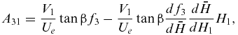 $$\begin{equation}
{A_{31}} = \frac{{{V_1}}}{{{U_e}}}\tan \beta {f_3} - \frac{{{V_1}}}{{{U_e}}}\tan \beta \frac{{d{f_3}}}{{d\bar{H}}}\frac{{d\bar{H}}}{{d{H_1}}}{H_1},
\end{equation}$$
$$\begin{equation}
{A_{31}} = \frac{{{V_1}}}{{{U_e}}}\tan \beta {f_3} - \frac{{{V_1}}}{{{U_e}}}\tan \beta \frac{{d{f_3}}}{{d\bar{H}}}\frac{{d\bar{H}}}{{d{H_1}}}{H_1},
\end{equation}$$
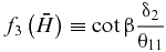 $$\begin{equation}
{f_3}\left( {\bar{H}} \right) \equiv \cot \beta \frac{{{\delta _2}}}{{{\theta _{11}}}}
\end{equation}$$
$$\begin{equation}
{f_3}\left( {\bar{H}} \right) \equiv \cot \beta \frac{{{\delta _2}}}{{{\theta _{11}}}}
\end{equation}$$
where δ 2 is defined in Equation (14)
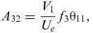 $$\begin{equation}
{A_{32}} = \frac{{{V_1}}}{{{U_e}}}{f_3}{\theta _{11}},\\
\end{equation}$$
$$\begin{equation}
{A_{32}} = \frac{{{V_1}}}{{{U_e}}}{f_3}{\theta _{11}},\\
\end{equation}$$
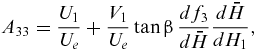 $$\begin{equation}
{A_{33}} = \frac{{{U_1}}}{{{U_e}}} + \frac{{{V_1}}}{{{U_e}}}\tan \beta \,\frac{{d{f_3}}}{{d\bar{H}}}\frac{{d\bar{H}}}{{d{H_1}}},\\
\end{equation}$$
$$\begin{equation}
{A_{33}} = \frac{{{U_1}}}{{{U_e}}} + \frac{{{V_1}}}{{{U_e}}}\tan \beta \,\frac{{d{f_3}}}{{d\bar{H}}}\frac{{d\bar{H}}}{{d{H_1}}},\\
\end{equation}$$
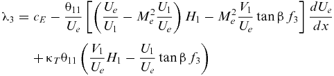 $$\begin{eqnarray}
{\lambda _3} &=& {c_E} - \frac{{{\theta _{11}}}}{{{U_e}}}\left[ {\left( {\frac{{{U_e}}}{{{U_1}}} - M_e^2\frac{{{U_1}}}{{{U_e}}}} \right){H_1} - M_e^2\frac{{{V_1}}}{{{U_e}}}\tan \beta \,{f_3}} \right]\frac{{d{U_e}}}{{dx}}\nonumber\\
&&+\, {\kappa _T}{\theta _{11}}\left( {\frac{{{V_1}}}{{{U_e}}}{H_1} - \frac{{{U_1}}}{{{U_e}}}\tan \beta \,{f_3}} \right)
\end{eqnarray}$$
$$\begin{eqnarray}
{\lambda _3} &=& {c_E} - \frac{{{\theta _{11}}}}{{{U_e}}}\left[ {\left( {\frac{{{U_e}}}{{{U_1}}} - M_e^2\frac{{{U_1}}}{{{U_e}}}} \right){H_1} - M_e^2\frac{{{V_1}}}{{{U_e}}}\tan \beta \,{f_3}} \right]\frac{{d{U_e}}}{{dx}}\nonumber\\
&&+\, {\kappa _T}{\theta _{11}}\left( {\frac{{{V_1}}}{{{U_e}}}{H_1} - \frac{{{U_1}}}{{{U_e}}}\tan \beta \,{f_3}} \right)
\end{eqnarray}$$
None of the equations above include the higher-order terms presented by Ashill et al(Reference Ashill, Wood and Weeks7) which appear in the Callisto governing equations. These are mainly concerned with improved modelling in regions of adverse pressure gradient and not included here as they have little impact upon the prediction of the flow near the AL.
One feature of the governing equations employed by Callisto which needs to be detailed is the different dependent variable used for the entrainment equation, the transformed shape factor H rather than H 1θ11, so that the governing equations appear as:
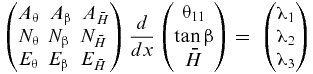 $$\begin{equation}
\left( {\begin{array}{@{}*{3}{c}@{}} {{A_\theta }}&\ {{A_\beta }}&\ {{A_{\bar{H}}}}\\ {{N_\theta }}&{{N_\beta }}&{{N_{\bar{H}}}}\\ {{E_\theta }}&{{E_\beta }}&{{E_{\bar{H}}}} \end{array}} \right)\frac{d}{{dx}}\left( {\begin{array}{@{}*{1}{c}@{}} {{\theta _{11}}}\\ {\tan \beta }\\ {\bar{H}} \end{array}} \right) = \;\left( {\begin{array}{@{}*{1}{c}@{}} {{\lambda _1}}\\ {{\lambda _2}}\\ {{\lambda _3}} \end{array}} \right)
\end{equation}$$
$$\begin{equation}
\left( {\begin{array}{@{}*{3}{c}@{}} {{A_\theta }}&\ {{A_\beta }}&\ {{A_{\bar{H}}}}\\ {{N_\theta }}&{{N_\beta }}&{{N_{\bar{H}}}}\\ {{E_\theta }}&{{E_\beta }}&{{E_{\bar{H}}}} \end{array}} \right)\frac{d}{{dx}}\left( {\begin{array}{@{}*{1}{c}@{}} {{\theta _{11}}}\\ {\tan \beta }\\ {\bar{H}} \end{array}} \right) = \;\left( {\begin{array}{@{}*{1}{c}@{}} {{\lambda _1}}\\ {{\lambda _2}}\\ {{\lambda _3}} \end{array}} \right)
\end{equation}$$
The left-hand side of Equation (A.1) can be written as
 $$\begin{equation}
{A_{11}}\frac{{d{\theta _{11}}}}{{dx}} + {A_{13}}\frac{d}{{dx}}\left( {{H_1}{\theta _{11}}} \right) = \left[ {{A_{11}} + {A_{13}}{H_1}} \right]\frac{{d{\theta _{11}}}}{{dx}} + {A_{13}}\left[ {{\theta _{11}}\frac{{d{H_1}}}{{d\bar{H}}}\frac{{d\bar{H}}}{{dx}}} \right]
\end{equation}$$
$$\begin{equation}
{A_{11}}\frac{{d{\theta _{11}}}}{{dx}} + {A_{13}}\frac{d}{{dx}}\left( {{H_1}{\theta _{11}}} \right) = \left[ {{A_{11}} + {A_{13}}{H_1}} \right]\frac{{d{\theta _{11}}}}{{dx}} + {A_{13}}\left[ {{\theta _{11}}\frac{{d{H_1}}}{{d\bar{H}}}\frac{{d\bar{H}}}{{dx}}} \right]
\end{equation}$$
This expansion can be repeated for the remaining normal-momentum and entrainment equations, so by inspection of Equation (A.20), the transformations from the variables used by Ashill and Smith to those used in Callisto can be written as:
 $$\begin{equation}
{A_\theta } = {A_{11}} + {A_{13}}{H_1}\quad {N_\theta } = {A_{21}} + {A_{23}}{H_1}\quad {E_\theta } = {A_{31}} + {A_{33}}{H_1},\\
\end{equation}$$
$$\begin{equation}
{A_\theta } = {A_{11}} + {A_{13}}{H_1}\quad {N_\theta } = {A_{21}} + {A_{23}}{H_1}\quad {E_\theta } = {A_{31}} + {A_{33}}{H_1},\\
\end{equation}$$
 $$\begin{equation}
{A_\beta } = {A_{12}}\quad {N_\beta } = {A_{22}}\quad {E_\beta } = {A_{32}},\\
\end{equation}$$
$$\begin{equation}
{A_\beta } = {A_{12}}\quad {N_\beta } = {A_{22}}\quad {E_\beta } = {A_{32}},\\
\end{equation}$$
 $$\begin{equation}
{A_{\bar{H}}} = {A_{13}}{\theta _{11}}\frac{{d{H_1}}}{{d\bar{H}}}\quad {N_{\bar{H}}} = {A_{23}}{\theta _{11}}\frac{{d{H_1}}}{{d\bar{H}}}\quad {E_{\bar{H}}} = {A_{33}}{\theta _{11}}\frac{{d{H_1}}}{{d\bar{H}}}
\end{equation}$$
$$\begin{equation}
{A_{\bar{H}}} = {A_{13}}{\theta _{11}}\frac{{d{H_1}}}{{d\bar{H}}}\quad {N_{\bar{H}}} = {A_{23}}{\theta _{11}}\frac{{d{H_1}}}{{d\bar{H}}}\quad {E_{\bar{H}}} = {A_{33}}{\theta _{11}}\frac{{d{H_1}}}{{d\bar{H}}}
\end{equation}$$
We also introduce the angle ψ between the direction of the inviscid streamline and the arc AC in Fig. 2.
 $$\begin{equation}
\frac{{{U_1}}}{{{U_e}}} = \cos \psi \quad \frac{{{V_1}}}{{{U_e}}} = \sin \psi
\end{equation}$$
$$\begin{equation}
\frac{{{U_1}}}{{{U_e}}} = \cos \psi \quad \frac{{{V_1}}}{{{U_e}}} = \sin \psi
\end{equation}$$
Following the change in independent variables, we obtain:
 $$\begin{equation}
{A_\theta } = {A_{11}} + {A_{13}}{H_1} = \cos \psi - \sin \psi \tan \beta \,{f_2},\\
\end{equation}$$
$$\begin{equation}
{A_\theta } = {A_{11}} + {A_{13}}{H_1} = \cos \psi - \sin \psi \tan \beta \,{f_2},\\
\end{equation}$$
 $$\begin{equation}
{A_{\bar{H}}} = {A_{13}}{\theta _{11}}\frac{{d{H_1}}}{{d\bar{H}}} = - \sin \psi \tan \beta \,\frac{{d{f_2}}}{{d\bar{H}}}{\theta _{11}},\\
\end{equation}$$
$$\begin{equation}
{A_{\bar{H}}} = {A_{13}}{\theta _{11}}\frac{{d{H_1}}}{{d\bar{H}}} = - \sin \psi \tan \beta \,\frac{{d{f_2}}}{{d\bar{H}}}{\theta _{11}},\\
\end{equation}$$
 $$\begin{equation}
{N_\theta } = {A_{21}} + {A_{23}}{H_1} = \tan \beta \left( {\cos \psi \,{f_1} - \sin \psi \tan \beta \,{f_4}} \right),\\
\end{equation}$$
$$\begin{equation}
{N_\theta } = {A_{21}} + {A_{23}}{H_1} = \tan \beta \left( {\cos \psi \,{f_1} - \sin \psi \tan \beta \,{f_4}} \right),\\
\end{equation}$$
 $$\begin{equation}
{N_{\bar{H}}} = {A_{23}}{\theta _{11}}\frac{{d{H_1}}}{{d\bar{H}}} = \tan \beta \left( {\cos \psi \frac{{d{f_1}}}{{d\bar{H}}} - \sin \psi \tan \beta \,\frac{{d{f_4}}}{{d\bar{H}}}} \right){\theta _{11}},\\
\end{equation}$$
$$\begin{equation}
{N_{\bar{H}}} = {A_{23}}{\theta _{11}}\frac{{d{H_1}}}{{d\bar{H}}} = \tan \beta \left( {\cos \psi \frac{{d{f_1}}}{{d\bar{H}}} - \sin \psi \tan \beta \,\frac{{d{f_4}}}{{d\bar{H}}}} \right){\theta _{11}},\\
\end{equation}$$
 $$\begin{equation}
{E_\theta } = {A_{31}} + {A_{33}}{H_1} = \cos \psi \,{H_1} + \sin \psi \tan \beta {f_3},\\
\end{equation}$$
$$\begin{equation}
{E_\theta } = {A_{31}} + {A_{33}}{H_1} = \cos \psi \,{H_1} + \sin \psi \tan \beta {f_3},\\
\end{equation}$$
 $$\begin{equation}
{E_{\bar{H}}} = {A_{33}}{\theta _{11}}\frac{{d{H_1}}}{{d\bar{H}}} = \left( {\cos \psi \frac{{d{H_1}}}{{d\bar{H}}} + \sin \psi \tan \beta \,\frac{{d{f_3}}}{{d\bar{H}}}} \right){\theta _{11}}
\end{equation}$$
$$\begin{equation}
{E_{\bar{H}}} = {A_{33}}{\theta _{11}}\frac{{d{H_1}}}{{d\bar{H}}} = \left( {\cos \psi \frac{{d{H_1}}}{{d\bar{H}}} + \sin \psi \tan \beta \,\frac{{d{f_3}}}{{d\bar{H}}}} \right){\theta _{11}}
\end{equation}$$
ACKNOWLEDGEMENTS
The authors would like to express their gratitude to the Aeromechanics team of Airbus Group Innovations for their financial support under agreement no. IW 10430.


