NOMENCLATURE

A

rotor disk area

B

number of blades

C _Q

rotor torque coefficient $${Q{\rm \,/\,}\left( {{\rrho }A{\rm \Omega }^{{\rm 2}} R^{{\rm 3}} } \right)}$$

C _P

rotor power coefficient $${P{\rm \,/\,}\left( {{\rrho }A{\rm \Omega }^{{\rm 3}} R^{{\rm 3}} } \right)}$$

C _T

rotor thrust coefficient $${T{\rm \,/\,}\left( {{\rrho }A{\rm \Omega }^{{\rm 2}} R^{{\rm 2}} } \right)}$$

c

local chord length

$${\bar{c}}$$

geometric mean chord length

c _d

profile drag coefficient

$${\bar{c}_{{\rm d}} }$$

blade averaged drag coefficient

c _l

profile lift coefficient

$${\bar{c}_{l} }$$

blade averaged lift coefficient

D _e

rotor’s equivalent drag at forward flight

F

McCormick correction function

k _ind

ratio between the ideal and actual induced power

r

radial distance from the hub

R

rotor disk radius

U

free stream axial velocity

u

induced axial velocity

u _m

mutual induced axial velocity

v

induced tangential velocity

v _m

mutual induced tangential velocity

W _e

equivalent velocity seen by the blade profile

x

axial distance

α

profile angle of attack

β

profile pitch angle

β_0.75

profile pitch angle at r=0.75R

λ_∞

tip speed ratio; $${U\,/\,\left( {{\rm \Omega }R} \right)}$$

μ

advance ratio of forward flight; $${U_{{{\rm hortizontal}}} \,/\,\left( {{\rm \Omega }R} \right)}$$

ρ

air density

σ

rotor solidity, $${B\bar{c}\,/\,\left( {{\rpi }R} \right)}$$

η_C

composite efficiency

Ω

rotor rotational speed

1.0 INTRODUCTION

Proprotors acting as rotors or propellers are commonly found in small unmanned aircraft (UAV). Unlike the large-scale rotors or propellers, these proprotors act in a low Reynolds number flow regime of less than Re_C of 3×10⁵ as based on the local chord length. Hence, the blade profiles are dominated by laminar boundary layers that are intolerant to high adverse pressure gradient, leading to early flow separation and stall as compared with the large-scale blades dominated by turbulent boundary layers⁽ Reference Mueller and DeLaurier ^{1 )}. This makes approaches that delay stall of particular interest for small UAV in terms of increasing propulsion performance and hence range and endurance.

Recently, the CIRCLE design method calling for continuous surface curvature and its derivative was used to redesign the NACA0012 and E387 profiles for low Re number flow⁽ Reference Shen, Avital, Rezaienia, Paul and Korakianitis ^{2 ,} Reference Shen, Avital, Paul, Rezaienia, Wen and Korakianitis ^{3 )}. The method name is the acronym of presCrIbed suRface Curvature distribution bLade dEsign (CIRCLE)⁽ Reference Korakianitis, Hamakham, Rezaienia, Wheeler, Avital and Williams ^{4 )}. It is based on designing the leading and trailing edges as rounded, i.e. circles or ellipses, albeit the trailing edge is of a much smaller circle. The edges are then connected using high-order polynomial and spline curves following the requirements of the profile thickness, but while keeping the surface curvature and its derivative continuous⁽ Reference Shen, Avital, Rezaienia, Paul and Korakianitis ^{2 )}. The procedure starts from the trailing edge, typically contoured as a circle with a radius of about 1.5% of the profile maximum thickness and continues building the profile towards the leading edge using the high-order polynomial and spline curves. Full details of the procedure are given in Shen et al.⁽ Reference Shen, Avital, Rezaienia, Paul and Korakianitis ^{2 )} and Korakianitis et al.⁽ Reference Korakianitis, Hamakham, Rezaienia, Wheeler, Avital and Williams ^{4 )}. It resulted in the new profiles QM13F and A7, replacing NACA0012 and E387, respectively. Redesigning the original spiky trailing edges of the NACA0012 and E387 to rounded trailing edges actually led to reduction in the production costs of the metal profiles⁽ Reference Shen, Avital, Paul, Rezaienia, Wen and Korakianitis ^{3 ,} Reference Shen, Avital, Zhao, Gao, Li, Paul and Korakianitis ^{5 )}.

In case of a highly twisted and swept blade as one may encounter in turbo-machinery, the surface curvature along the blade span can also be of interest and the CIRCLE design approach has been expanded for 3D bodies as was done for subsonic and transonic compressor blades⁽ Reference Korakianitis, Hamakham, Rezaienia, Wheeler, Avital and Williams ^{4 )}. However, the typical blade for a proprotor of a small UAV is straight and moderately twisted. Hence, any discontinuity in the surface curvature will usually be at the profile’s plane. Therefore, this study will concentrate on adopting 2D profiles designed using the CIRCLE method for use in a proprotor.

The CIRCLE method’s root for requiring continuous surface curvature in order to yield smooth pressure variation along the profile can be found in Van Dykes’ second-order thin aerofoil theory⁽ Reference Shen, Avital, Rezaienia, Paul and Korakianitis ^{2 )}. It was found to yield a delay in the burst of the leading edge separation bubble and thus a delay in the stall of thin aerofoil at high angle-of-attack (AOA). This was confirmed by RANS and Large Eddy Simulations (LES) carried using Ansys⁽ Reference Shen, Avital, Rezaienia, Paul and Korakianitis ^{2 ,} Reference Shen, Avital, Paul, Rezaienia, Wen and Korakianitis ^{3 )} and our in-house code CgLES⁽ Reference Shen, Avital, Zhao, Gao, Li, Paul and Korakianitis ^{5 )}. It was also further validated using detailed wind tunnel tests⁽ Reference Shen, Avital, Paul, Rezaienia, Wen and Korakianitis ^{3 )}. The behaviour is demonstrated in Fig. 1, showing the lift and drag coefficients c _l and c _d variations as taken from Shen et al.⁽ Reference Shen, Avital, Rezaienia, Paul and Korakianitis ^{2 ,} Reference Shen, Avital, Paul, Rezaienia, Wen and Korakianitis ^{3 )}. At low AOA, the CIRCLE design approach was experimentally and computationally found to reduce the laminar separation bubble (LSB) over the profile’s upper surface and thus mildly reduce the drag and significantly reduce the tonal trailing edge noise by up to 10 dB⁽ Reference Shen, Avital, Paul, Rezaienia, Wen and Korakianitis ^{3 ,} Reference Shen, Avital, Zhao, Gao, Li, Paul and Korakianitis ^{5 )}. The noise reduction occurred due a decrease in the LSB size which resulted in suppressing its interaction with the trailing edge and its flapping. In this study, we will concentrate on the aerodynamic performance improvement due to the use of the CIRCLE-based blade profile in low Re number single and co-axial proprotors and leave the aeroacoustic effect for a future study.

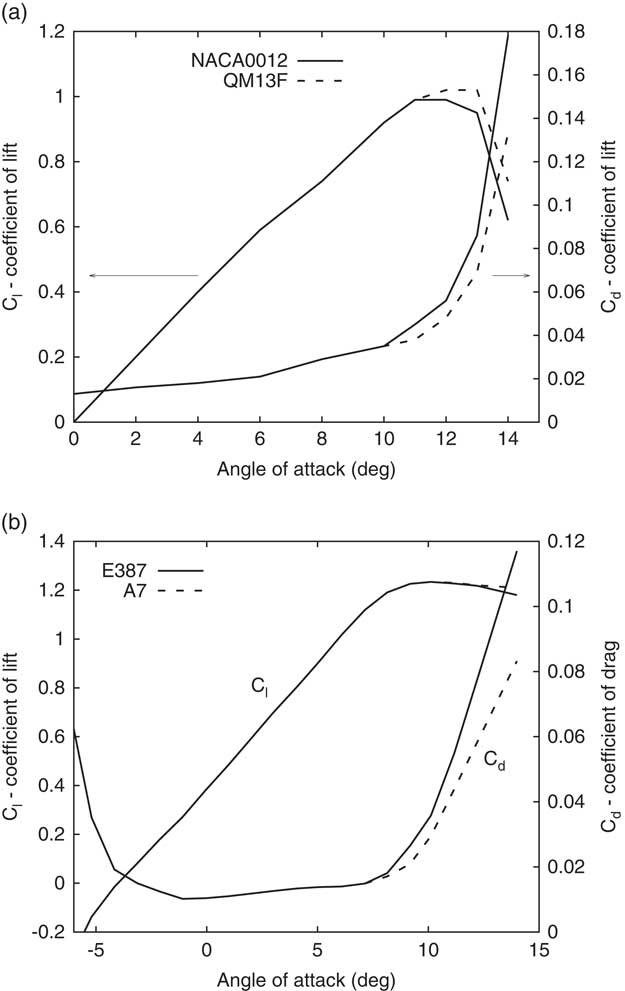
Figure 1 The lift and drag coefficients variations with the angle of attack that are plotted for the profiles: (a) NACA0012 and the CIRCLE-redesigned QM13F of Re_D=1.35×10^{5 (} Reference Shen, Avital, Rezaienia, Paul and Korakianitis ^{2 )} and (b) E387 and the CIRCLE-redesigned A7 of Re_D=2×10^{5 (} Reference Shen, Avital, Paul, Rezaienia, Wen and Korakianitis ^{3 )}.

The delay in the stall of the A7 profile as compared with the E387 profile was shown to yield about 10% increase in the power of a small wind turbine operating at a range of Re_C=200k and high AOA⁽ Reference Shen, Avital, Paul, Rezaienia, Wen and Korakianitis ^{3 )}. Thus, it is of interest to investigate its effect on proprotors. This is not just due to the small UAV application but also due to growing interest in propeller-driven propulsion for near space vehicles⁽ Reference Zhang, Yang, Song and Song ^{6 )} as well as in extraterrestrial thin atmospheres as on Mars, where the Reynolds number is also expected to be low. Asymmetric profiles as the E387 are commonly used for propellers, where symmetric profiles are more commonly used for rotors. Hence, both are investigated here for proprotor applications.

Traditionally, propeller aerodynamic performance has been analysed using the blade element method and/or models based on the vortex theory⁽ Reference Wald ^{7 )}. This holds whether the propeller is of large scale or small scale, although the aerodynamic data for the blade profiles have to be adjusted accordingly, while also taking into account effects as compressibility and swept blades⁽ Reference Zhang, Yang, Song and Song ^{6 ,} Reference Wald ^{7 )}. The blade element method has been proved to be a mature rapid analysis tool of good accuracy⁽ Reference Gur and Rosen ^{8 )}. More computational intensive tools as computational fluid dynamics (CFD) are also available and can provide higher accuracy and better insight into the flow regime development around the blade⁽ Reference Korakianitis, Hamakham, Rezaienia, Wheeler, Avital and Williams ^{4 )}, particularly when a turbulent flow simulation as LES is pursued⁽ Reference Bai, Avital, Munjiza and Williams ^{9 )}. However, CFD tools are much more computationally expensive than the blade element method approach.

While the blade element method whether coupled with the momentum theory or vortex theory is a mature approach to analyse a single proprotor, it is less developed for the counter-rotating (co-axial) configuration. Such configuration has been investigated since World War II and is particularly attractive as a rotor system to achieve balanced torque. The swirl from the front rotor is used to increase the AOA on the rear rotor blade and thus to mitigate some of the adverse effect of a higher incoming axial velocity also induced by the front rotor. The torque balance of the co-axial proprotor can be achieved by changing the rear blade pitch angle as in this study, but also by changing the rotor’s rotational speed that is much easier to implement by electric motors commonly used in drones than by gas turbines used in larger aircraft. A summary of aerodynamic models used to analyse the co-axial proprotor during the decades after WWII is given in Playle et al.⁽ Reference Playle, Korkan and Lavante ^{10 )}.

Recently, Leswisham⁽ Reference Leishman ^{11 )} elegantly extended the blade element momentum theory (BEMT) to the co-axial configuration assuming low AOAs and achieving good agreement with several experimental results. A simpler 1D model was developed by Beaumier⁽ Reference Beaumier ^{12 )}, but both models could not explicitly account for the distance between the rotors. An attempt to account for that distance was given by Juhasz et al.⁽ Reference Juhasz, Syal, Celi, Khromov, Rand, Ruzicka and Strawn ^{13 )}, who empirically extended the McCormick’s formula of the axial velocity at the centreline induced by a helical vortex⁽ Reference McCormick ^{14 )}. A new approach to explicitly account for the effect of the distance between the two rotors in the co-axial configuration is derived in this study using previous results of the generalised actuator disk⁽ Reference Hough and Ordway ^{15 )}. It also accounts for large AOAs experienced by the blade profile as expected near stall.

To summarise, the aim of this study is to investigate the effect of CIRCLE-designed profiles of a continuous surface curvature on the aerodynamic performance of single and co-axial proprotors. To achieve this, the methodology is given in the next section. It is followed by analysis based on general arguments of composite efficiency and rotor’s lift to drag ratio in order to assess the effect of the new profile. Aerodynamic analysis of several single and co-axial proprotors is also pursued and is followed by the Summary section.

2.0 THE PROBLEM DESCRIPTION AND METHODOLOGY

This study concentrates on a single or a co-axial rotor in static or axial translation conditions. These proprotors can be viewed as helicopter rotors or aircraft propellers, depending on their design, but all can be schematically described as in Fig. 2(a) and (b). Because we concentrate on low Reynolds number applications as found in small UAV, incompressibility assumption will be used. Hence, straight blades will also be assumed. Extension to account for compressibility and swept back blades is possible⁽ Reference Zhang, Yang, Song and Song ^{6 ,} Reference Playle, Korkan and Lavante ^{10 )} and can be implemented in a future study.

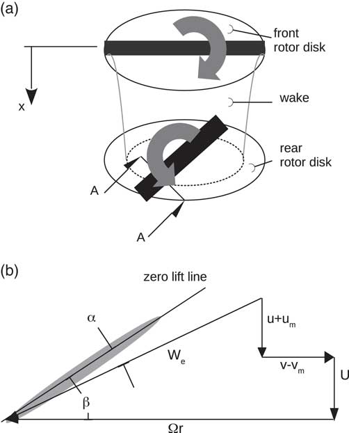
Figure 2 Schematic description of the co-axial proprotor.

Traditionally, propellers have been analysed using the blade element method approach while being coupled with the momentum method or a vortex model⁽ Reference Wald ^{7 ,} Reference Beaumier ^{12 )}. Although CFD methods are capable of providing detailed insight into the physics of the flow, they are computationally expensive as already noted. This particularly holds for the counter-rotating (co-axial) rotor where an unsteady flow simulation as URANS or LES has to be implemented. Thus, for this study, the blade element method has been used, which has been shown to provide accurate results for steady loads⁽ Reference Gur and Rosen ^{8 )}. This is except for post-stall conditions where improvement in rotor power modelling is needed⁽ Reference Morgado, Silvestre and Pascoa ^{16 )}. Nevertheless, the trend using the CIRCLE-designed profile is still clear as will be discussed in the Results section.

The BEMT approach that was developed by Leishman⁽ Reference Leishman ^{11 )} to deal with the co-axial proprotor relied on the assumption of small angles of attack (AOAs), while most of the improvement due to the CIRCLE design is in high AOA. Therefore, the McCormick vortex model as coupled with the blade element method is used⁽ Reference McCormick ^{14 )}:

(1) $${{{{4\rpi }r} \over B}F(r)v(r){\equals}{{\rm 1} \over {\rm 2}}c(r)c_{l} (r)W_{{\rm e}} (r)}$$

where r is the distance from the hub. F is McCormick’s correction factor that is similar to the Prandtl tip loss factor⁽ Reference McCormick ^{14 )}. v is the induced tangential velocity by the rotor on itself. c is the local chord length. c _l is the profile lift coefficient and W _e is the equivalent velocity, see Fig. 2(b). F will be taken as of a single rotor. It is an approximation, but the analysis of Beaumier⁽ Reference Beaumier ^{12 )} and Leishman⁽ Reference Leishman ^{11 )} has been successful in analysing each rotor as a single rotor while accounting for the effect of the other rotor just through the mutual induced velocities u _m and v _m as is done next. Furthermore, our model has shown good agreement with Leishman BEMT⁽ Reference Leishman ^{11 )} for low AOAs and with experimental results as discussed in the next section.

Equation (1) is coupled with the following geometrical relations from Fig. 2(b):

(2) $${u{\plus}u_{{\rm m}} {\equals}{{\rm 1} \over {\rm 2}}\left\{ {{\minus}U{\plus}\left[ {U^{{\rm 2}} {\plus}{\rm 4}\left( {v{\minus}v_{{\rm m}} } \right)\left( {{\rm \Omega }r{\minus}v{\plus}v_{{\rm m}} } \right)} \right]^{{{\rm 1}\,/\,{\rm 2}}}} \right\} }$$

and

(3) $${{\rm tan}\left( {{\rbeta }{\minus}{\rm \ralpha }} \right){\equals}{{U{\plus}u{\plus}u_{{\rm m}} } \over {{\rm \Omega }r{\minus}v{\plus}v_{{\rm m}} }}}$$

The signs of Ω and v _m have been adjusted for the counter-rotating configuration. If c _l(α) and c _d(α) are known, then Equations (1)–(3) can be solved for v using a non-linear equation solver, provided that the mutual induced velocities u _m & v _m are known. The solution for v, will also yield the value for the induced axial velocity u from Equation (2).

In the BEMT model, v _m=0 on the rear rotor, while Leishman⁽ Reference Leishman ^{11 )} took u _m of the rear rotor as twice of u at the front rotor, i.e. the rear rotor is the far field of the front rotor. Jushaz et al.⁽ Reference Juhasz, Syal, Celi, Khromov, Rand, Ruzicka and Strawn ^{13 )} used an empirical correction to McCormick’s formula⁽ Reference McCormick ^{14 )} for the axial distribution of u at the centre-line of a semi-infinite helical vortex sheet of radius R:

(4) $${{{u(x)} \over {u(x{\equals}{\rm 0})}}{\equals}{\rm 1}{\plus}\left( {{{x\,/\,R} \over {\sqrt {{\rm 1}{\plus}(x\,/\,R)^{{\rm 2}} } }}} \right)^{k} }$$

k=1 at the centre-line r=0⁽ Reference McCormick ^{14 )}, while it decays with the radius to about 0.3 at r=R ⁽ Reference Juhasz, Syal, Celi, Khromov, Rand, Ruzicka and Strawn ^{13 )}.

In this study, we will assume that the rear rotor is in the slip stream of the front rotor and will use the actuator disk theory of Hough & Ordway⁽ Reference Hough and Ordway ^{15 )} that showed the steady velocity field u(x,r) to be linearly dependent on an integral of the circulation contained in the disk. Assuming a uniform circulation, the distribution of u(x,r) was calculated by them and is repeated in Table 1, where x=0 denotes the location of the disk and x>0 points downstream of the disk. As seen u(x=0,r) is uniform for r<R and u(x,r=0) follows Equation (4) when taking k=1. On the other hand, the radial change in u is less than 20% for r<R and u becomes close to zero for r>R.

Table 1 Normalized axial velocity u/(U C _T) distribution as induced by an actuator disk of blade constant circulation⁽ Reference Hough and Ordway ^{15 )}

Hence, the following procedure is proposed to calculate the mutual induced velocities u _m & v _m on the rear rotor. Calculate u & v on the front rotor using the McCormick model outlined above or any blade element method, while neglecting the effect of the rear rotor, i.e. u _m=v _m=0 on the front rotor. This will result in knowing u & v for N radial elements of the front rotor (disk). Proceed to calculate u _m on the rear rotor as follows:

Step 1: Take the induced axial velocity u(x=0, r=r _N) and assume that it is the same all over the front disk. Use Equation (4) to calculate the axial distribution of u(x,r) by assuming u(x,r)=u(x) for r<R, i.e. neglect the radial variation of u, which we will call model 0. Alternatively, use Table 1 to calculate u(x,r) as relative to u(x=0, r=r _N) which we will call as model 1. In both models, we approximate u(x,r>R)=0. The omission of any induced velocity outside the disk’s stream-tube was investigated by Spalart⁽ Reference Spalart ^{17 )} to show it to be an accurate approximation, where also the change in the stream-tube from a state of climb of the rotor to descent was also investigated. Store the value of u(x,r) at the axial location of the rear disk.

Step 2: Subtract u(x=0, r=r _N ) from the distribution of u(x=0, r). This will result in a smaller disk of radius (r _N−1+r _N )/2. Repeat Step 1 but for the new hypothetical velocity $${\tilde{u}\left( {x{\equals}{\rm 0},r{\equals}r_{{N{\minus}{\rm 1}}} } \right)}$$ which is u(x=0, r=r _N−1) −u(x=0, r=r _N ). Add the contribution of u at the rear rotor to the previous value.

Step 3: Repeat Steps 2 and 1 until all radial elements of the front disk were accounted. One should note that during this process, the hypothetical velocity $${\tilde{u}\left( {x{\equals}{\rm 0},r} \right)}$$ on the front disk may become negative. In that case switch between the downstream and upstream directions in Equation (4) or Table 1.

The induced tangential velocity v _m can be calculated through angular momentum conservation, i.e. v(x=0, r _front-rotor) r _front-rotor=v(x _rear-rotor, r _rear-rotor) r _rear-rotor. To find the relation between r _rear-rotor and r _front-rotor, the mass conservation rule is used. The induced flux q(r) on the front rotor is found by integrating u(x=0,r) and similarly q _m(r) on the rear rotor by integrating u _m(r) that was just found. Then, the relation between r _rear-rotor and r _front-rotor is found by matching q(r) with q _m(r). In this step, we assumed that q(r) is monotonically increasing, i.e. u(x=0, r)≥0, so the AOA is positive. This has happened in the examples discussed in the next section. If u(x=0, r)<0, then the recommendation is to omit the contribution of v _m following Leishman⁽ Reference Leishman ^{11 )}.

After calculating u _m & v _m on the rear rotor, its u & v can be calculated using the McCormick vortex model detailed earlier or any other blade element method. An iterative procedure may be initiated to calculate u _m & v _m on the front rotor using a similar procedure as for the rear rotor. However, v _m on the front rotor is expected to be very small due to the fast decay of the swirl upstream and can be approximated as zero⁽ Reference Beaumier ^{12 )}. Our numerical experience has shown that for the kind of co-axial rotors investigated here, there is no merit in pursuing such iterative approach to find u _m on the front rotor and it was taken as zero. This is also supported by the BEMT approach that neglects u _m on the front rotor⁽ Reference Leishman ^{11 )}.

The coefficients of thrust and power of each rotor can be calculated as follows⁽ Reference McCormick ^{14 )}:

(5) $${C_{{\rm T}} {\equals}\mathop{\int}\limits_{\rm 0}^{\rm 1} {{{{\rsigma }W_{{\rm e}}^{{\rm 2}} } \over {\left{\rm 2}( {{\rm \Omega }R} \right)^{{\rm 2}} }}\left[ {c_{l} {\rm cos}\left( {{\rbeta }{\minus}{\ralpha }} \right){\minus}c_{{\rm d}} {\rm sin}\left( {{\rbeta }{\minus}{\ralpha }} \right)} \right]{\rm d}x} }$$

(6) $${C_{{\rm P}} {\equals}\mathop{\int}\limits_{\rm 0}^{\rm 1} {{{{\rsigma }xW_{{\rm e}}^{{\rm 2}} } \over {\left{\rm 2}( {{\rm \Omega }R} \right)^{{\rm 2}} }}\left[ {c_{l} {\rm sin}\left( {{\rbeta }{\minus}{\ralpha }} \right){\plus}c_{{\rm d}} {\rm cos}\left( {{\rbeta }{\minus}{\ralpha }} \right)} \right]{\rm d}x} }$$

McCormick’s vortex model requires a non-linear equation solver as well as the usual requirement to balance the torque between the front and rear rotors. This can be done by varying the rear rotor rotational speed and blade pitch angle, where for the examples discussed in the next section, it was sufficient just to vary the blade pitch angle. The robust bi-section method was used as the non-linear solver with the two loops: the inner loop for solving McCormick’s model and the outer loop to balance the torque.

Finally, a stall-delay model due to rotational augmentation was implemented following Dumirescu and Cardos⁽ Reference Dumitrescu and Cardos ^{18 )}:

(7) $${c_{l} {\equals}c_{{l,{\rm 2d}}} {\plus}\left( {c_{{l,{\rm inv}}} {\minus}c_{{l,{\rm 2d}}} } \right)\left[ {{\rm 1}{\minus}{\rm e}^{{{\minus}{\rm 1}{\rm .25}\,/\,\left( {r\,/\,c{\minus}{\rm 1}} \right)}} } \right]}$$

where c _l,2d is the c _l of the 2D blade profile, c _l,inv is the 2D profile lift coefficient if no separation occurred, where in this study, it was taken as of inviscid theory, r is the radial distance from the hub and c is the local chord length. Further improvement can be achieved by also correcting the profile drag coefficient c _d, but currently such models usually result only in a mild improvement in the thrust prediction and no noticeable improvement in the power prediction⁽ Reference Morgado, Silvestre and Pascoa ^{16 )}.

3.0 RESULTS AND ANALYSIS

3.1 General arguments

Stepniewski and Keys⁽ Reference Stepniewski and Keys ^{19 )} provided two general measures to check the effect of a blade profile aerodynamics on a single rotor performance. The first measure is the figure of merit (FM) which is the ratio between the ideal power to the actual power in static (hover) condition. The second measure is the ratio between the helicopter’s rotor lift to its equivalent drag during forward flight. The FM measure can be extended to axial translation of the rotor using the composite efficiency measure⁽ Reference Leishman ^{11 )}:

(8) $${{\reta }_{c} {\equals}{{C_{{\rm T}} {\rm \lambda }_{\infty} {\plus}C_{{{\rm P,id}}} } \over {C_{{\rm T}} {\rm \lambda }_{\infty} {\plus}C_{{{\rm P,ind}}} {\plus}C_{{{\rm Pr}}} }}}$$

where $${{\rm \lambda }_{\infty} {\equals}U\,/\,\left( {{\rm \Omega }R} \right)}$$ is the tip speed ratio (TSR). C _P,id is the ideal induced power coefficient, i.e. assuming uniform induced axial velocity and no tip losses. C _P,ind is the actual induced power coefficient and C _Pr is the profile power coefficient. In the case of a co-axial rotor, the C _P’s are contributed by the front and rear rotors, e.g. C _P,ind=C _P,ind,front+C _P,ind,rear, assuming the same ΩR for both rotors.

Assuming $${{\rm \Omega }r\,\gg\,U{\plus}u}$$ and neglecting the effect of v, one can show by following the Appendix that for a single rotor:

(9) $${{\reta }_{c} {\equals}{{{\rm 3\lambda }_{\infty} {\plus}\sqrt {{\rm \lambda }_{\infty}^{{\rm 2}} {\plus}{\rsigma }\bar{c}_{l} \,/\,{\rm 3}} } \over {{\rm 2\lambda }_{\infty} {\plus}\left( {{\rm \lambda }_{\infty} {\plus}\sqrt {{\rm \lambda }_{\infty}^{{\rm 2}} {\plus}{\rsigma }\bar{c}_{l} \,/\,{\rm 3}} } \right)k_{{{\rm ind}}} {\plus}{\rm 3}\bar{c}_{{\rm d}} \,/\,\left( {{\rm 2}\bar{c}_{l} } \right)}}}$$

where k _ind is C _P,ind/C _P,id. $${\tilde{c}_{l} }$$ and $${\tilde{c}_{{\rm d}} }$$ are the blade’s averaged coefficients of lift and drag, respectively, and σ is the solidity of the rotor. Equation (9) converges to the FM expression of Stepniewski and Keys⁽ Reference Stepniewski and Keys ^{19 )} when taking the tip speed ratio λ_∞=0.

The variations of the composite efficiency for static conditions, rotor solidity σ=0.1 and TSR of 0.1 according to Equation (9) are given in Figs 3 and 4 for the symmetric profiles NACA0012 & QM13F and the asymmetric profiles E387 & A7. QM13F & A7 are the CIRCLE re-designed profiles and the profile aerodynamic performance was taken from Fig 1(a) and (b). To account for the AOAs well after stall, post-stall empirical relations were implemented^{( 20 )}. This resulted in the gradient kinks seen in the curves, particularly for the NACA0012 & QM12F at AOA≈15⁰ in Fig. 3(a) and (b). Nevertheless, the improvement due to the re-designed profiles at high AOAs is very clear in both static and axial translation. Increases of at least 10% in efficiency can be observed as well as wider curves of maximum efficiency and thus providing more flexibility to the aerodynamic designer.

Figure 3 The figure of merit variations with the profile angle of attack that are plotted for generic single rotor disks having the profiles: (a) NACA0012 or QM13F and (b) E387 or A7 of Fig 2. k _ind – the ratio of actual to induced ideal power equally varies from 1.1 to 1.5.

Figure 4 The composite efficiency variations with the profile angle-of-attack that are plotted for the generic rotor disks of Fig. 3 at axial translation with a tip speed ratio of λ_∞=0.1.

A general expression for the ratio of a single rotor lift L to its equivalent drag D _e at forward flight was given by Stepniewski and Keys⁽ Reference Stepniewski and Keys ^{19 )}:

(10) $${{L \over {D_{{\rm e}} }}{\equals}{{\rm 1} \over {\left( {{\rsigma }k_{{{\rm ind}}} \bar{c}_{l} } \right)\,/\,\left( {{\rm 12\mu }^{{\rm 2}} } \right){\plus}{\rm 3}\left( {{\rm 1}{\plus}{\rm 4}{\rm .7\mu }^{{\rm 2}} } \right)\bar{c}_{{\rm d}} \,/\,\left( {{\rm 4\mu }\bar{c}_{l} } \right)}}}$$

and is plotted in Fig. 5 for all four investigated profiles and advance flight ratio μ=0.3. Again the CIRCLE re-designed profiles QM13F and A7 outperform the original NACA0012 and E387 profiles at high AOAs, respectively. This is caused by the better aerodynamic efficiency at high AOA. Interestingly, the asymmetric profiles show L/D _e higher than the symmetric profiles, indicating their efficiency when it comes to moderate advance flight ratio. The rest of this section concentrates on rotors or propellers in static and axial translation conditions.

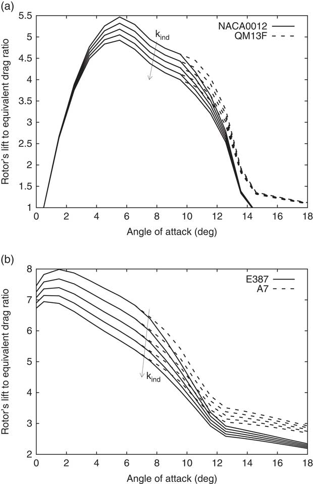
Figure 5 The rotor’s lift to equivalent drag ratio variations with the profile angle of attack that are plotted for the generic rotor disks of Fig. 3 and at horizontal flight with an advance speed ratio μ=0.3.

3.2 The co-axial rotor

The counter-rotating Harrington rotors have been commonly used as a test case due to their detailed experimental results⁽ Reference Harrington ^{21 )}. These are two-blades rotors, where Rotor 1 is of a tapered chord and thickness blade and Rotor 2 is of a tapered thickness blade. Both blades are untwisted and their profiles are NACA00XX where the XX stands for the profile thickness ratio.

The variations of the thrust coefficient C _T with the torque coefficient C _Q are plotted in Fig. 6 for both rotors in static conditions, where the chord Reynolds number at r=0.75R was of about 1M, and the profile aerodynamic data was adjusted accordingly⁽ Reference Sheldahl and Kilmas ^{22 )}. One should note that for the co-axial rotor, the front and rear rotors were torque balanced and thus C _Q is twice of the front rotor. Excellent agreement is revealed between our method and the experimental results for both the single and co-axial rotors. For the co-axial Rotor 1, not much difference is revealed between Model 0 and Model 1 that differ in calculating the radial variation of u _m along the rear rotor. However, for co-axial Rotor 2, Model 1 that better accounts for the radial variation of u _m outperforms Model 0.

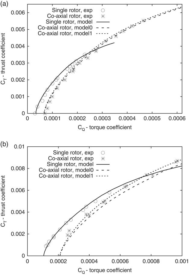
Figure 6 Variations of the thrust and torque coefficients of the Harrington two-blade rotors’ static-thrust tests⁽ Reference Harrington ^{21 )} and which are plotted for (a) Rotor 1 of the tapered chord and thickness blade and (b) Rotor 2 of the tapered thickness blade. Model 0 means u(x,r)=u(x, r=0) of Table 1 for r<R. Model 1 means u(x,r) is found using Table 1.

To examine the effect of replacing NACA0012 with QM13F, Rotor 2 was rescaled for the Reynolds number of Re_C=1.35×10⁵ as in Fig. 1(a) and modified to have a uniform profile of NACA 0012 or QM13F. This means the blade is uniform in chord length, thickness and c _l & c _d variations with the AOA. It is an approximation of a hypothetical rotor that aims to investigate the difference between the two profiles and not to provide exact results for a particular rotor. The variation of the figure of merit with the overall thrust coefficient is shown in Fig. 7 for the single and co-axial rotor configurations. The QM13F-based rotors show improved FM at high C _T due to the improved aerodynamic efficiency of QM13F at high AOA. The improvement is more noticeable in the co-axial rotor than in the single rotor.

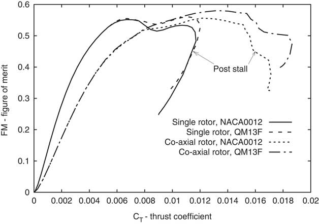
Figure 7 The variation of the figure of merit with the static thrust coefficient for a small re-scaled Harrington Rotor 2, where the blade profile is uniformly NACA0012 or QM13F of Fig. 1(a).

To better understand the effect of changing the NACA0012 profile with the QM13F profile, contours of the aerodynamic efficiency c _l /c _d are plotted in Fig. 8 as a function of the radial location and the blade pitch angle of the front rotor. As the mutual induced velocities u _m & v _m are neglected in the front rotor calculation, the contours for the front rotor should also be viewed as for the single rotor.

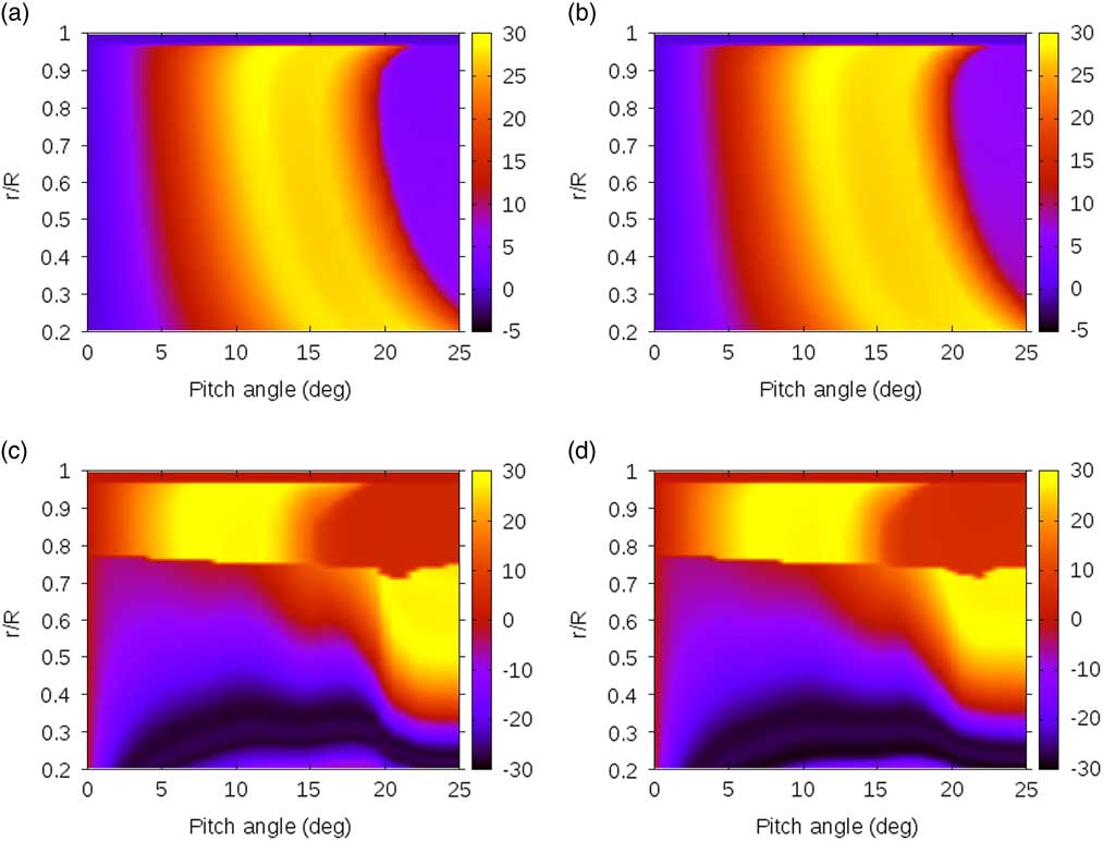
Figure 8 The spanwise variation of the blade profile’s lift to drag ratio for the range of untwisted blade pitch angle β corresponding to the FM plots of Fig. 7 and which are plotted for (a) the upper rotor with the NACA0012 profile, (b) the upper rotor with the QM13F profile, (c) the lower rotor with the NACA0012 profile and (d) the lower rotor with the QM13F.

It is seen that the front rotor’s regime of reduced aerodynamic efficiency at high-pitch angle is mildly mitigated in the QM13F profile as compared to the NACA0012 profile, thus resulting in the moderate improvement in the FM of the single rotor seen in Fig. 7. The rear rotor shows two opposite patterns of behaviour. The area of r>(0.7–0.8)R that is outside of the wake shed by the front rotor. It shows a behaviour similar to that of the front rotor, i.e. increase in the aerodynamic efficiency with the pitch angle until stall has reached and then a decrease in the aerodynamic efficiency due to post stall condition. The area that is inside the front rotor wake of r<(0.7–0.8)R shows low aerodynamic efficiency at low pitch angles because of the high u _m caused by the front rotor which reduces the AOA on the rear rotor. However, at high-pitch angle, the front rotor stalls and u _m is much reduced causing the AOA to increase on the rear rotor for r<(0.7–0.8)R as seen in Fig. 8(b) and (d). The sharp border in Fig. 8(c) and (d) around r=0.75R, is obviously an approximation of the wake effect, similar to the approach used in Leishman’s⁽ Reference Leishman ^{11 )} proprotor model for when the rear rotor was in the far field of the front rotor’s wake. Nevertheless, the model yields accurate results as seen in Fig. 6. On overall, the co-axial rotor based on the QM13F profile outperforms the NACA0012-based co-axial rotor in high-pitch angles, i.e. high thrust coefficient as seen Fig. 7.

The variation of the composite efficiency with the tip speed ratio (TSR) for the small rescaled rotor is shown in Fig. 9 for both the single and co-axial configurations. As the TSR increases, the AOA seen by the blade profile decreases and thus the difference between the QM13F and NACA0012-based blades diminishes. Hence, the highest difference is at static condition for a fixed pitch angle, where the composite efficiency becomes the figure of merit of Fig. 7. Interestingly, the composite efficiency initially increases for the co-axial rotor and high-pitch angle of 18° as the TSR is increased from zero. This is related to the behaviour of the rear rotor as seen in Fig. 8.

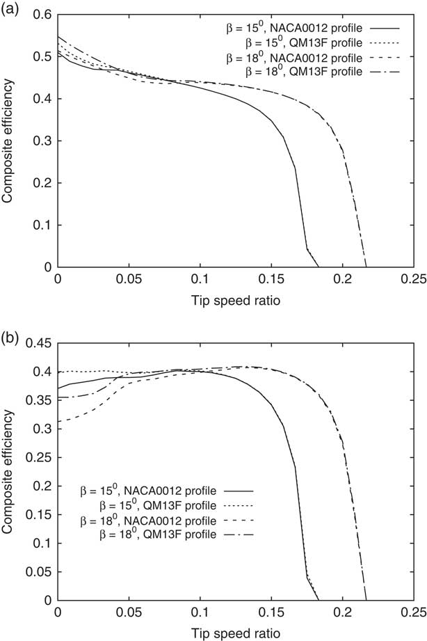
Figure 9 Variation of the composite efficiency η_C with the tip speed ratio λ_∞ for the small rescaled (a) single and (b) co-axial Harrington Rotor 2, where both are at axial translation and β is the untwisted blade pitch angle.

3.3. The single low Reynolds number propeller

Symmetric profiles as the NACA0012 are commonly used for rotors, while asymmetric profiles are more commonly used for propellers. Experimental measurements were provided by Ghoddoussi⁽ Reference Ghoddoussi ^{23 )} and his small-scale two blade COMP propeller based on the E387 was picked up for this study. The variations of the thrust and power coefficients with the TSR are given in Fig. 10, where for the model, the c _l&c _d variations were based on Re_C=10⁵. For consistency, the experimental propeller results were re-adjusted for the definitions of the thrust and power coefficients, and tip speed ratio as commonly used for rotor aerodynamics and that are used in this study.

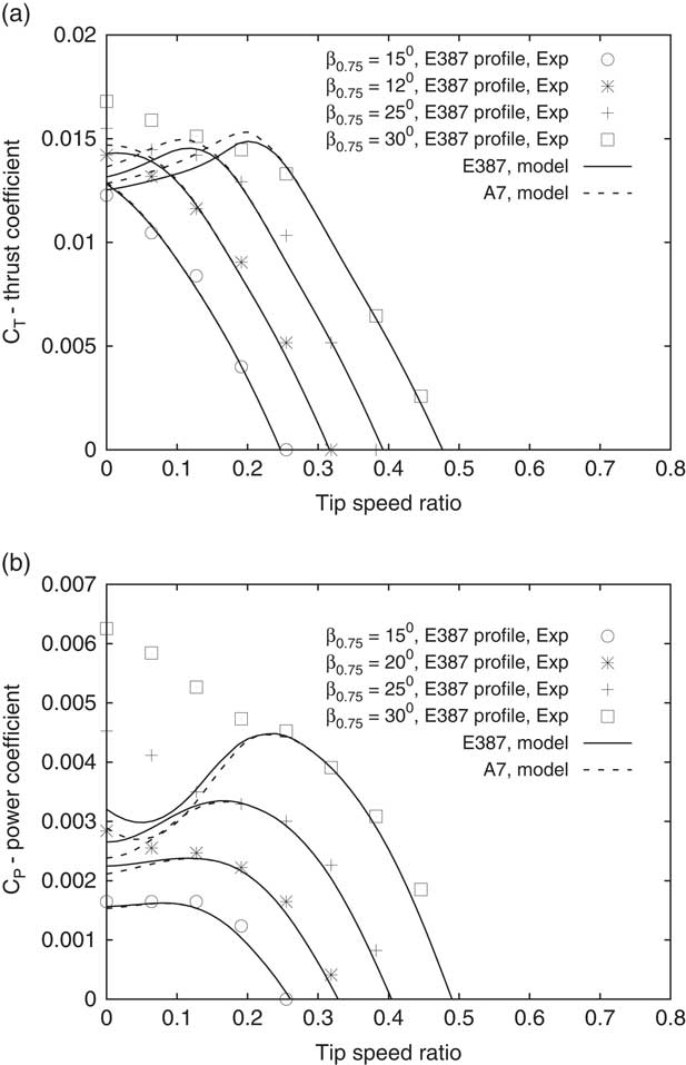
Figure 10 The variations of the (a) thrust and (b) power coefficients for the two-blade twisted COMP propeller having the E387 profile⁽ Reference Ghoddoussi ^{23 )} and the redesigned A7 profile.

Very good agreement is revealed between the experimental and model results for high TSR or low blade pitch angle, where both the E387 and A7 propellers give the same result. This is because of the low AOAs seen by the propeller blades. At high-pitch angles and low TSR, big differences can be seen between the experimental and model results, particularly for C _P. This is because of the current inadequacy of stall-delay models to accurately predict the power⁽ Reference Morgado, Silvestre and Pascoa ^{16 )}, pointing to the need to improve such models. Nevertheless, the trend caused by replacing E387 by the redesigned A7 is consistent and clear. It results in a higher C _T and a lower C _P for low TSRs and high-pitch angles. This is as expected from the better aerodynamic efficiency of the A7 at high AOA, pointing to the benefit in using the CIRCLE-based profile,

4.0 SUMMARY

Two low Reynolds number redesigned blade profiles QM13F and A7 were investigated for their effect on thrust and power of single and co-axial proprotors. The QM13F is a redesign of the NACA0012 profile and the A7 is a redesign of the E387 profile. Both redesigns followed the CIRCLE procedure calling for a continuous surface curvature and its derivative along the profile. Previously published results of c _l & c _d verses AOA of both profiles for Re_C<3×10⁵ were used and coupled with a blade-element method based on the McCormick vortex model. To model the co-axial rotor, the rear rotor was assumed to be in the slipstream of the front rotor. A new method as based on the generalised actuator disk theory was proposed to account for the effect of the distance between the rotors, leading to a formulated approach to calculate the mutual induced velocities acting on the rear rotor. For the investigated co-axial rotor configurations, it was found to be sufficient to neglect the mutual induced velocity on the front rotor.

General arguments were used to produce analysis based on the composite efficiency measure at axial translation and rotor’s lift to equivalent drag at forward flight. This was followed by blade element method analysis of several single and co-axial proprotors, leading to the following conclusions:

• ∙ The blade element method coupled with the McCormick method and the new approach to account for the distance between the rotors of a co-axial configuration produced excellent agreement with experimental results in terms of thrust and torque/power. However, the need for imported stall-delay models was highlighted for highly stalled blades and particularly for the power prediction.

• ∙ The higher aerodynamic efficiency of the CIRCLE-based blade at high AOA leads to a wider envelope of high efficiency and more flexibility for the aerodynamic designer.

• ∙ The performance improvement was more noticeable in the co-axial configuration than the single configuration due to the behaviour the rear rotor blade. The blade produced high aerodynamic efficiency at the slip stream region of the front rotor after the latter stalled. This is because of a reduction in u _m acting on the rear rotor.

Straight and moderately twisted blades were considered in this study as one may expect for proprotors of small UAVs. However, as already noted, when highly twisted and swept blades are used, discontinuities in the surface curvature may occur along the blade’s span and the CIRCLE approach should be applied three-dimensionally as it was in turbo-machinery applications⁽ Reference Korakianitis, Hamakham, Rezaienia, Wheeler, Avital and Williams ^{4 )}. This study concentrated on the aerodynamics of the proprotor, but as noted earlier the CIRCLE-based profile can yield a reduced tonal self-aerofoil noise at the low Reynolds numbers studied here. To what degree it affects the overall noise generation by the proprotor that includes other components of noise as the thrust-torque noise and wake noise is an open research question.

Appendix

The composite efficiency, general approximation

The thrust coefficient C _T and the ideal power coefficient C _P,id of a single rotor can be taken as

(A.1) $${C_{{\rm T}} {\equals}{\rm 2\lambda }_{{{\rm id}}} \left( {{\rm \lambda }_{\infty} {\plus}{\rm \lambda }_{{{\rm id}}} } \right),\quad C_{{{\rm P,id}}} {\equals}{C}_{T} \left( {{\rm \lambda }_{\infty} {\plus}{\rm \lambda }_{{{\rm id}}} } \right)}$$

where $${{\rm \lambda }_{{{\rm id}}} {\equals}u_{{{\rm id}}} \,/\,\left( {{\rm \Omega }R} \right)}$$ and $${{\rm \lambda }_{\infty} {\equals}U\,/\,\left( {{\rm \Omega }R} \right)}$$ ⁽ Reference Stepniewski and Keys ^{19 )}. u _id is the ideal uniform induced axial velocity. The ratio between the axial induced power and the ideal power is defined as k _ind=C _P,ind/C _P,id. Assuming $${{\rm \Omega }r\,\gg\,U{\plus}u}$$ and thus low flow angle β−α, one gets that;

(A.2) $${C_{{{\rm Pr}}} {\equals}{\rsigma }\bar{c}_{{\rm d}} \,/\,{\rm 8},\quad C_{{\rm T}} {\equals}{\rsigma }\bar{c}_{l} \,/\,{\rm 6}}$$

Substituting Equations (A.1) and (A.2) into the expression of the composite efficiency in Equation (8) leads to the general expression of Equation (9), after expressing λ_id as a function of λ_∞ and the blade’s averaged lift coefficient $${\bar{c}_{l} }$$ .