


1.0 Introduction
Recent years have witnessed a demand for sustainable aviation [Reference Argüelles, Lumdsen, Bischoff, Ranque, Busquin, Rasmussen, Droste, Reutlinger, Evans, Robins, Kröll, Terho, Lagardère, Wittlöv and Lina1]. This led to the greener-by-design concept, which involves low acoustic noise and low drag aircraft. One way to reduce drag is to use laminar flow technology [Reference Schrauf2]. The development of low noise aircraft and laminar flow technology both benefit from wind tunnels with low background acoustic noise and low turbulence [Reference Eckert, Mort and Jope3–Reference Cattafesta, Bahr and Mathew6]. It is within this context that the wind tunnel here introduced, the Low Acoustic Noise and Turbulence (LANT) wind tunnel, was designed and built.
Table 1 shows a comprehensive list of wind tunnels that have been used for aerodynamic, stability and/or aeroacoustic studies. For comparisons, the LANT characteristics are also shown. Such tunnels were selected because their dimensions, speed range, flow characteristics or applications are similar to the wind tunnel addressed in this paper.
Table 1. Characteristics of selected wind-tunnel facilities. Abbreviations: N/A (information not available), CS (closed section), OS (open section), CL (closed-loop), OL (open loop), S (screen), H (honeycomb), AN (anechoic chamber), KW (kevlar-walled), AM (absorbing material), C (circuit), TS (test section), AA (aeroacoustic), AD (aerodynamic), ST (stability). *but has provision

The closed-loop configuration is the dominant design among the facilities in Table 1. Among other benefits, closed-loop requires less power to drive the fan, which reflects in less fan noise. It also permits a better control of flow temperature, which is important for several applications. As the temperature has a strong effect on the air viscosity and hence Reynolds number, for experiments in flow instability with controlled excitations, a variation of temperature is very inconvenient because it also leads to a variation in the physical frequency of the unstable modes. On the other hand, such tunnels tend to overheat at high speeds. We note that most of the closed section and circuit facilities reported in Table 1 that are designed for stability experiments have a cooling circuit or provision for installation of a heat exchanger, e.g. NDF (3), ALSWT (8), MTL (10), EC (11), BUWT (12), PCT (18) and F2 (25). In LANT this effect is more severe because the acoustic treatment constitutes a thermal isolation, and this is the reason the current results are limited to 30 m/s. In the list, wind tunnels for flow stability studies have a closed working section, while those for aeroacoustics studies often have an open working section within an anechoic chamber. There are a few wind tunnels featuring the possibility of open and closed sections, e.g. FSAT (5), PCT (18), DNW-NWB (19) and D5 (31), in some cases for stability or aeroacoustic experiments, e.g. FSAT (5), PCT (18).
The open design in combination with the anechoic chamber prevents sound reverberation in the working section, which is essential for single microphone measurements. However, open-section wind tunnels have great difficulty in establishing the far-field boundary conditions of the flow around the model, in particular for lift-generating models [Reference Kröber52, Reference Amaral, Pagani, Himeno, Souza and Medeiros53]. This has led to the Kevlar wall working section design [Reference Devenport, Burdisso, Borgoltz, Ravetta, Barone, Brown and Morton7, Reference Remillieux, Crede, Camargo, Burdisso, Devenport, Rasnick, Van Seeters and Chou8, Reference Devenport, Bak, Brown and Borgoltz29, Reference Smith, Camargo, Burdisso and Devenport54], which aims at providing an effective wall for the flow and at the same time a transparent wall for the acoustic waves. This design provided a noticeable improvement in the experiments. At the same time, studies have shown that judicious use of beamforming techniques reduce reverberation effects, and working section wall acoustic treatment brings extra benefits [Reference Syms18, Reference Fischer and Doolan38, Reference Sijtsma and Holthusen55–Reference Amaral and Pagani60]. This strategy led to very good comparisons between experiments and simulations [Reference Pagani, Souza and Medeiros61–Reference Souza, Rodríguez, Himeno and Medeiros64]. Based on the above discussion, we decided for a wind tunnel design of closed return and closed working section.
Among the studied facilities, Table 1, only six wind tunnels give information of background acoustic noise, with only two in a closed working section. From these two, LAE-1 (37) is not a low turbulence tunnel, while KSWT (2), is a reference tunnel for stability experiments. KSWT (2) presents a higher background noise than LAE-1, however, LAE-1 used a much higher high-pass filter, which in general massively reduces these figures. The measurements were performed with a single microphone placed in the working section.
All tunnels addressed in Table 1 present turbulence-intensity levels. However, in a wind tunnel the dominant flow fluctuations are of low frequency, and the turbulence intensity measurement is severely affected by filtering the low frequency, content. The frequency range used varied wildly among the tunnels, and some tunnels do not mention the frequency range used. Because of that, we relied on wind tunnels that had a long history of research in flow stability, namely, the Gaster’s wind tunnel (15), currently located at City University (UK), the KSWT (2), located at Texas A&M (USA) and the MTL (10), of the KTH (Sweden), which provided detailed information about turbulence intensity. From Table 1 it is seen that, apart from the Gaster’s wind tunnel (15), the other tunnels do not appear among the lower turbulence levels reported. We believe that this may in part be attributed to the different methods of turbulence-level quantification. The spectrum of turbulence is also very important information, which is rarely given. The Gaster’s wind tunnel (15) and the KSWT (2) provide this information. MTL (10) provides turbulence-level distribution in the test section cross section.
Just under a third of these tunnels provide measurements of flow uniformity. The numbers vary substantially, and the values depend on uniformity definition and the region covered. For instance, many assessments of flow uniformity are made along a line and not over an area. Ideally one would like to have a picture of the flow distribution over the useful area of the tunnel, but only a few references provide it. KSWT (2) and MTL (15) provide detailed information about flow uniformity.
Based on this background information, our approach for the design of the Low Acoustic Noise and Turbulence (LANT) wind tunnel was to use design best practices employed in stability wind tunnels, which have low turbulence, adding specific provisions for acoustic noise control. Aeroacoustic wind tunnels are commonly derived from the facilities designed to conduct aerodynamic experiments adapted for low background acoustic noise [Reference Devenport, Burdisso, Borgoltz, Ravetta, Barone, Brown and Morton7, Reference Hunt, Downs, Kuester, White and Saric9, Reference Devenport, Bak, Brown and Borgoltz29]. Other efforts convert originally anechoic facilities into aeroacoustic wind tunnels [Reference Mathew, Bahr, Sheplak, Carroll and Cattafesta13]. In this respect, from the point of view of aeroacoustic wind tunnels, our design approach is innovative.
Best practices used in low-turbulence wind tunnels are not entirely established. Hence, a number of decisions had to be made when conflicting strategies were found; among them, we highlight the following. Short settling chambers run the risk of interference between the upstream effects of contraction and the screens, an aspect that is difficult to estimate a priori. On the other hand, long contractions produce thick boundary layers, which reduce the useful area in the working section, a very important issue for a relatively small-section wind tunnel. In fact, most wind tunnels use a short settling chamber. The distance between screens is another issue over which there is no consensus, some claiming that a rather long distance is needed. Our approach was to use a long settling chamber for the reason discussed above but also because this is one aspect that is sure to reduce freestream turbulence. To further lengthen the settling chamber, we used relatively small distances between screens. To compensate the boundary layer growth, a short contraction was used. The shorter distance reduces the opportunity for boundary layer growth, and, more importantly, the strong favourable pressure gradient prevents boundary layer growth. This comes with a risk of boundary layer separation, which was controlled in the design technique used. The resulting boundary layer thickness and turbulence level in the working settling indicates that this is an interesting strategy.
The design specifications established for the LANT wind tunnel were: (1) a top speed of 30 m/s, with power provision to raise this number to up to 60 m/s, in which case temperature control would be implemented; (2) working section area
 $1 \times 1\ \textit{m}^2$
and 3 m length; (3) turbulence intensity level below 0.1% (in the frequency range given by the dynamic filter introduced by Lindgren and Johansson [Reference Lindgren and Johansson20]); (4) flow uniformity within 1%; (5) closed section acoustic background noise below 110 dB in the frequency range 1 to 10,000 Hz; and (6) the above conditions should hold in a cross-section larger than
$1 \times 1\ \textit{m}^2$
and 3 m length; (3) turbulence intensity level below 0.1% (in the frequency range given by the dynamic filter introduced by Lindgren and Johansson [Reference Lindgren and Johansson20]); (4) flow uniformity within 1%; (5) closed section acoustic background noise below 110 dB in the frequency range 1 to 10,000 Hz; and (6) the above conditions should hold in a cross-section larger than
 $800 \times 800$
mm
$800 \times 800$
mm
 $^2$
.
$^2$
.
In this paper we address several aspects of the LANT wind tunnel. It is organised as follows. After this introduction, Section 2 discusses the design criteria and construction details of the wind tunnel. In Section 3, flow characterisation results for the empty test section are reported, whereas Section 4 provides results of benchmark experiments. Finally, Section 5 summarises the conclusions.
2.0 Design
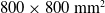
Figure 1 shows the facility aerodynamic circuit solution obtained to meet the desired requirements, and Table 2 summarises the geometrical characteristics of the wind tunnel sections. The facility is 18.5-m long
 $\times$
8.7-m wide
$\times$
8.7-m wide
 $\times$
3.7-m high.
$\times$
3.7-m high.
Table 2. Wind-tunnel aerodynamic circuit main characteristics. L is the section length,
 $\theta$
the section divergence angle and CR is the contraction ratio
$\theta$
the section divergence angle and CR is the contraction ratio

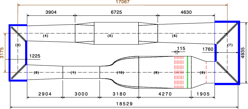
Figure 1. LANT wind tunnel aerodynamic circuit plan view. (1) test section, (2) first diffuser, (3) first and second corners, (4) second diffuser, (5) fan, (6) third diffuser, (7) third and fourth corners, (8) wide angle diffuser, (9) settling chamber and (10) contraction. Dimensions in millimetres. The thick blue lines at the first, second, third and fourth corners indicate the acoustic treatment. At the settling chamber, the dashed red lines indicate the screens (there is also a screen just before the wide-angle diffuser) and the green hatched rectangle indicate the honeycomb.
The table also presents the pressure loss coefficient
 $K_i$
, for each tunnel component, defined as
$K_i$
, for each tunnel component, defined as
 \begin{equation} K_i = \frac{\Delta P_i}{\frac{1}{2} \rho U^2} \mbox{,} \end{equation}
where U and
 $\rho$
, are the empty test section air speed and the density, respectively. The total circuit loss,
$\rho$
, are the empty test section air speed and the density, respectively. The total circuit loss,
 $\Delta P_{\rm total}$
is
$\Delta P_{\rm total}$
is
 \begin{equation} \Delta P_{\rm total} = \sum {\Delta P_i} \mbox{,} \end{equation}
where
 $\Delta P_i$
is the pressure drop in each component normalised by the dynamic pressure at the test section, with flow velocity
$\Delta P_i$
is the pressure drop in each component normalised by the dynamic pressure at the test section, with flow velocity
 $U = 30$
m/s and
$U = 30$
m/s and
 $\rho = 1.225$
kg/m
$\rho = 1.225$
kg/m
 $^3$
. Sections pressure drops were estimated by methods well-established in the literature [Reference Cattafesta, Bahr and Mathew6, Reference Bradshaw65–Reference Barlow and Rae67]. The percentile contribution to the total pressure loss is also provided. The settling chamber, which contains the screens and the honeycomb, represents approximately 1/3 of the aerodynamic circuit losses.
$^3$
. Sections pressure drops were estimated by methods well-established in the literature [Reference Cattafesta, Bahr and Mathew6, Reference Bradshaw65–Reference Barlow and Rae67]. The percentile contribution to the total pressure loss is also provided. The settling chamber, which contains the screens and the honeycomb, represents approximately 1/3 of the aerodynamic circuit losses.
A modular design was chosen for easy transport and replacement of any of the components. About half the tunnel, including the working section, is located in a clean room, where the instrumentation is housed. The other half is in a hangar and permits easy access for fan and screen maintenance. The flat wind tunnel walls were manufactured with 15-mm thick water-resistant plywood panels. A layer of primer coat was applied on the plywood panels. After the wall assembly, emery paper was employed to smooth the surfaces and level the plywood panels joints. Finally, a coat of paint was applied for protection against humidity. The contraction walls were manufactured in fibreglass. For preventing leaking, a 5-mm thick
 $\times$
50-mm wide flexible rubber sealant was employed at each tunnel module joint. The tunnel walls were supported and structured by 50-mm edge and 1.5-mm thick SAE 1020 steel rebars.
$\times$
50-mm wide flexible rubber sealant was employed at each tunnel module joint. The tunnel walls were supported and structured by 50-mm edge and 1.5-mm thick SAE 1020 steel rebars.
The following subsections give details of each component of the facility aerodynamic circuit.
2.1 Fan
The axial fan, with 1.8 and 0.68 m external and hub diameters, respectively, is driven by an 110 kW Siemens electric motor. This excessive power was chosen for future extension to higher speeds, as per Fig. 2. The rotor blades were manufactured in fibreglass and reinforced with steel bars. The fan included a stator, also with fibreglass blades. Figure 2 exhibits the required fan power as a function of the test section flow speed, based on the pressure drops in Table 2.
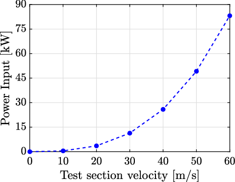
Figure 2. Fan power as a function of the test section freestream speed.
The fan design aimed at minimising the noise generation. The fan is a significant source of acoustic background noise [Reference Rumsey, Biedron, Farassat and Spence68] usually classified in two different contributions [Reference Huff69]: a broadband noise and discrete frequency noise. The noise is generated either by the rotor (rotor self-noise) or the stator, or by the interaction between them [Reference Fukano, Kodama and Senoo70]. The broadband noise is produced by the turbulence in the blade boundary layers, vortex shedding at the blades trailing edge, interactions between the blades, random turbulence in the intake flow [Reference Sharland71], among others. Noise associated with blade tip clearance is often the most important of broadband nature [Reference Rumsey, Biedron, Farassat and Spence68]; the unsteady tip vortex interacts with the rotor blades trailing edge, and, downstream, hits the stator blades. In our design the tip clearance was kept below 20 mm.
The fan rotation governs the formation of discrete noise tones. It generates noise at the blades passing frequency (BPF) and its harmonics, which can propagate both downstream and upstream. They are called spinning modes. The waveguide theory permits to establish which modes propagate (the higher frequency modes) and which modes decay (the lower frequency ones). Tyler and Sofrin [Reference Tyler and Sofrin72] applied this theory to the design of rotor and stator fans. Their model defines the propagating modes for a given stator and rotor number of blades and fan rotation and establishes which of them propagate or decay. Using this theory, we obtained that a 16-blade rotor and a 13-blade stator prevented the propagation of the lowest frequency acoustic waves that would be generated by the rotor-stator interaction, which is the most undesirable mode.
In order to minimise structural vibrations and transfer to other parts of the tunnel circuit, the fan was mounted on a large and isolated concrete slab, with a steel plate attached to the bottom of the structure and secured by anchor rods. Rubber pads were sandwiched between the plates and the floor. The fan module was isolated from the second and the third diffusers through a 100-mm wide flexible coupling.
The flow produced by the fan has a significant residual rotational component with high levels of turbulence and very poor uniformity. Most of the other wind tunnel components are designed to reduce such undesirable characteristics of the flow.
2.2 Diffusers
The diffusers are employed to enlarge the flow area from the smallest tunnel section (the working section) to the widest one (the settling chamber). To prevent flow separation on its walls, which would induce low-frequency fluctuations and turbulence in the test section, each diffuser had an equivalent cone angle of less than 5 deg and the inlet-to-outlet cross-sectional area ratio was less than 2.5 [Reference Mehta73]. For maintenance, access doors were provided in a vertical wall of each diffuser.
To reduce the length of the wind tunnel that would otherwise be required in view of the used contraction ratio, a wide angle diffuser was placed just upstream of the settling chamber. In such diffusers, flow separation can only be avoided through boundary layer control [Reference Mehta73]. The most common method to avoid the flow separation in wide angle diffusers is inlet screens, which were used here. Based on Mehta [Reference Mehta73], it was found that only one screen was needed for separation control, with the same characteristics of those employed in the settling chamber, Section 2.4. According to Mehta [Reference Mehta73], the diffuser inlet is the best location for the screen. We took as confirmation that the wide-angle diffuser is fully working the fact that the boundary-layers at the test-section walls are relatively thin, the non-uniformities are low and that no low-frequency content that scaled with tunnel speed and could then be associated with some kind of boundary layer separation was observed, as will be addressed in Sec. 3.
2.3 Corners
At each tunnel corner, turning vanes are need to prevent flow separation, reducing pressure loss. The air-conditioning industry developed very efficient devices that are used in large ducts, which reached the standards required for wind tunnel. They are for instance used on the KSWTFootnote 1 . In the LANT, Ductmate acoustical turning vanes filled with acoustic foam and specially designed for quiet installations were employed. They are constructed in an aluminium alloy. The vane pressure side has a porous surface, and the profile is filled with an acoustic absorbent material. The profile chord and spacing between the vanes are 82.55 mm (3-1/4”) and 101.6 mm (4”), respectively.
The corners internal walls were coated with recessed 100-mm thick BASF acoustic melamine-based foam to absorb soundFootnote 2 . Black polyurethane film was applied on the foam surface to prevent erosion due to the airflow and, according to the manufacturer, to further improve the noise absorption. The thickness of a layer of an acoustic absorbing material should be at least a quarter of the wavelength of the lowest frequency of interest. [Reference Cox and D’antonio74] Hence, the chosen foam is effective for frequencies higher than approximately 1,000 Hz.
2.4 Settling chamber
The 4.3-m long settling chamber is equipped with one honeycomb and up to seven screens, but in the current tests, five screens were used. The honeycomb primary objective is to remove any residual flow swirls and its length to diameter ratio (
 $L_{HC}/D_{HC}$
) should be at least 10 cell diameter for optimal reduction of swirl. [Reference Loehrke and Nagib75, Reference Saric and Reshotko76] The aluminium 63.5-mm thick honeycomb had a 3.175 mm diameter hexagonal-shaped cells (
$L_{HC}/D_{HC}$
) should be at least 10 cell diameter for optimal reduction of swirl. [Reference Loehrke and Nagib75, Reference Saric and Reshotko76] The aluminium 63.5-mm thick honeycomb had a 3.175 mm diameter hexagonal-shaped cells (
 $L_{HC}/D_{HC} = 20$
). A stainless steel 1.587 mm diameter wires were stretched at the downstream face of the honeycomb to hold it in place. It is important to ensure that the flow in the honeycomb cell is laminar. [Reference Loehrke and Nagib75] For the tunnel future top speed (60 m/s), the cell diameter 3.175 mm leads to a Reynolds number of approximately 2,000. For easy cleaning and maintenance, a rail and drawer mechanism was designed to dock the screens and honeycomb on the settling chamberFootnote
3
. The wide-angle diffuser screen was also placed in a drawer. The drawers also provided the means for tensioning the screens in placeFootnote 4.
$L_{HC}/D_{HC} = 20$
). A stainless steel 1.587 mm diameter wires were stretched at the downstream face of the honeycomb to hold it in place. It is important to ensure that the flow in the honeycomb cell is laminar. [Reference Loehrke and Nagib75] For the tunnel future top speed (60 m/s), the cell diameter 3.175 mm leads to a Reynolds number of approximately 2,000. For easy cleaning and maintenance, a rail and drawer mechanism was designed to dock the screens and honeycomb on the settling chamberFootnote
3
. The wide-angle diffuser screen was also placed in a drawer. The drawers also provided the means for tensioning the screens in placeFootnote 4.
Groth and Johansson [Reference Groth and Johansson77] demonstrated that the turbulence intensity downstream of a set of screens is primarily given by the last screen. They also say that, for the same level of turbulence, a reduced pressure drop is obtained by a set of progressively finer screens, as long as the scale of the incoming turbulence is substantially larger than the mesh size. However, in our tunnel, the honeycomb establishes a turbulence scale upstream of the screens, and, under these circumstances, it is recommended that the screens are 5–15 times finer than the honeycomb, [Reference Saric and Reshotko76] which leads to screen mesh size of 0.6 mm maximum. It is hard to find a low solidity screen with such a small cell, and, in any case, it would be very fragile. In view of that, we decided for a set of constant mesh nylon screens with a mesh size M of 1.26 mm, which is close to the recommendations by Saric and Reshotko, [Reference Saric and Reshotko76] and a wire diameter of 0.31. Groth and Johansson [Reference Groth and Johansson77] demonstrated that combinations of 2 slightly supercritical screen provide levels of turbulence similar to what would be achieved by a subcritical screen, with the added benefit of a lower pressure drop. It their tests,
 $Re_d$
(Reynolds number based on wire diameter) was 65. In our case,
$Re_d$
(Reynolds number based on wire diameter) was 65. In our case,
 $Re_d = 88$
at 30 m/s, which is not far from Groth and Johansson [Reference Groth and Johansson77]. At 60 m/s,
$Re_d = 88$
at 30 m/s, which is not far from Groth and Johansson [Reference Groth and Johansson77]. At 60 m/s,
 $Re_d = 177$
, it is possible the turbulence intensity will be higher.
$Re_d = 177$
, it is possible the turbulence intensity will be higher.
Bradshaw and Pankhurst [Reference Bradshaw and Pankhurst78] recommends a screen porosity above 0.57, whereas Groth and Johansson [Reference Groth and Johansson77] above 0.5. Reduced porosity is critical for transition experiments in boundary layer as it can severely affect boundary layer spanwise uniformity. [Reference Mehta73] The screen used had a porosity of
 $\beta_{s}$
of 0.57, and, as shown later, provided a very uniform boundary layer. Saric and Reshotko [Reference Saric and Reshotko76] recommend a distance between screens of at least 250 mesh sizes, however, Groth and Johansson [Reference Groth and Johansson77] demonstrated that a rapid decay of turbulence occurs within 25 screen cells downstream. After that, the decay is slower and linear with distance. Following Groth and Johansson [Reference Groth and Johansson77] results, our strategy was not to try and take advantage of the linear decay between screens, which could be lost in following screen, and trade it for extra room for linear decay downstream of the last screen. For construction reasons our screen had to be at least 150 mm (120 screen mesh size) apart. In any case, in the current configuration with five screens, the first three screens are separated by 230 mm (180 screen mesh size), close to Saric and Reshotko [Reference Saric and Reshotko76] recommendation. We decided to provide this larger separation for the first screens because they receive a larger scale and higher-level turbulence and are more likely to benefit fully from the linear decay between screens.
$\beta_{s}$
of 0.57, and, as shown later, provided a very uniform boundary layer. Saric and Reshotko [Reference Saric and Reshotko76] recommend a distance between screens of at least 250 mesh sizes, however, Groth and Johansson [Reference Groth and Johansson77] demonstrated that a rapid decay of turbulence occurs within 25 screen cells downstream. After that, the decay is slower and linear with distance. Following Groth and Johansson [Reference Groth and Johansson77] results, our strategy was not to try and take advantage of the linear decay between screens, which could be lost in following screen, and trade it for extra room for linear decay downstream of the last screen. For construction reasons our screen had to be at least 150 mm (120 screen mesh size) apart. In any case, in the current configuration with five screens, the first three screens are separated by 230 mm (180 screen mesh size), close to Saric and Reshotko [Reference Saric and Reshotko76] recommendation. We decided to provide this larger separation for the first screens because they receive a larger scale and higher-level turbulence and are more likely to benefit fully from the linear decay between screens.
After the last screen there is still residual turbulence that can only decay with time. For this reason, we opted for a longer settling chamber. Many tunnels have a very short settling chamber, e.g. approximately 2.5 m in the MTL wind tunnel (10) at KTH. [Reference Lindgren and Johansson20] Other low turbulence reference tunnels (e.g. the KSWT facility (2) at Texas A&M) have a settling chamber length after the screen section in the range of 0.7–1 of the settling chamber height (they are square section tunnels). Here we used a length of approximately 1.6 times the chamber height. Short settling chambers may cause an interference between the potential flow upstream effects of contraction and the screens. This conflict is, however, difficult to evaluate a priori, in particular because of the screens, but is addressed in the next section. On the other hand, long-settling chambers offer an opportunity for boundary layer growth which reduce the useful area in the working section. In fact, most wind tunnels use a short settling chamber. This issue was of great concern for our relatively small-section wind tunnel. Our approach was to use a long-settling chamber as this would also reduce freestream turbulence as discussed above. To compensate the boundary layer growth a short contraction was used, as addressed in the next section.
2.5 Contraction
The contraction design was based on a method developed by Whitehead et al. [Reference Whitehead, Wu and Waters79], which was also employed in the Gaster’s wind tunnel (15)Footnote 5 . In a contraction, between two parallel-wall ducts, there are two regions with adverse pressure gradient, at the inlet and outlet. Long contractions tend to reduce the magnitude of these undesirable gradient. The method developed by Whitehead et al. [Reference Whitehead, Wu and Waters79] permits to limit the magnitude of the adverse pressure gradient in a contraction, while keeping the contraction as short as possible and ensuring an uniform velocity shortly after the contraction. It uses a hodograph plane in which the velocity is specified along the contraction wall and the contraction shape is obtained from an integral equation. Such a fast contraction minimises the boundary layer thickness on the working section walls, which is very important for a small test cross-section wind tunnel. Small boundary layers also tend to reduce background acoustic noise and flow turbulence. Corner fillets initiate in the settling chamber just downstream from the last screen, reach a maximum of 150 mm at the contraction inlet and vanish at the contraction outlet.
There is concern about longer settling chambers, because they allow a long wind tunnel wall for boundary layer growth. This is in part compensated by our short contraction. The total length between the last screen and the test section inlet in our tunnel is 6 m while other figures are approximately 5.5 m for the MTL (10) and 7.3 m for the KSWT (2). The short contraction also subjects the boundary layer to a highly favourable pressure gradient, which reduces boundary layer thickness. In some tunnels, it is claimed that the boundary layer relaminarises in the contraction and that a trip has to be placed to avoid separation. In our tunnel, we verified that the flow was attached at the contraction, and for this reason no trip was used.
The short contraction design used is also optimal in the sense that, theoretically, it has the least impact in upstream flow uniformity and offers the shortest return to flow uniformity. In other words, if asked how far upstream, owing to potential flow effects, the contraction distorts an uniform flow by say 1%, and far downstream the flow has already return to uniformity within 1%; theoretically this contraction offers the shortest distance between this two points. An such distances are about one upstream contraction height for the distance upstream, and one downstream contraction height for the distance downstream. If the effect upstream stretches to a long distance and the settling chamber is short there will be conflict between the screens and the contraction. The screens may force a uniform flow at a point where the contraction is already distorting the flow. This conflict tends to further distort the flow downstream of the contraction towards the test section.
2.6 Test section
The 3 m long test section has 1 m width
 $\times$
1 m height inlet and 1.02 m width
$\times$
1 m height inlet and 1.02 m width
 $\times$
1 m height outlet cross-sectional area dimensions. Here the wall divergence aimed at keeping the flow speed constant along the working section by compensating for the working section wall boundary layer growth, which, otherwise would accelerate the flow in the streamwise direction. Regarding the wall divergence, based on information from other tunnels, we assumed a boundary layer of
$\times$
1 m height outlet cross-sectional area dimensions. Here the wall divergence aimed at keeping the flow speed constant along the working section by compensating for the working section wall boundary layer growth, which, otherwise would accelerate the flow in the streamwise direction. Regarding the wall divergence, based on information from other tunnels, we assumed a boundary layer of
 $\delta = 100$
mm at the working section entrance for a speed of 30 m/s and using Blasius correlation for a turbulent boundary layer at zero pressure gradient, we estimated the growth along the working section. For the range of speeds between 15 and 60 m/s, we obtained variations of
$\delta = 100$
mm at the working section entrance for a speed of 30 m/s and using Blasius correlation for a turbulent boundary layer at zero pressure gradient, we estimated the growth along the working section. For the range of speeds between 15 and 60 m/s, we obtained variations of
 $\delta^*$
between 4 and 5 mm, from which we estimated the 20 mm divergence for each vertical wall. The measurements carried out for the assessment of the flow quality revealed the assumption of
$\delta^*$
between 4 and 5 mm, from which we estimated the 20 mm divergence for each vertical wall. The measurements carried out for the assessment of the flow quality revealed the assumption of
 $\delta = 100$
mm was reasonable.
$\delta = 100$
mm was reasonable.
Four interchangeable 10 mm thick Plexiglass windows supported on aluminium frames allows easy access. Two floor/ceiling Plexiglass wall panels are also available, aiming at providing optical access for video cameras and/or laser beams. A vent was installed at the test section outlet to induce room pressure at this point. Wheels and quick-fit mechanisms enable the uncoupling of the test section from the wind tunnel, facilitating test model installation and test section exchange.
2.7 Traverse mechanism
In order to accurately move and position a probe, a stepper motor’s traverse mechanism was specially designed and built to suit the LANT test section dimensions. It is optimised for boundary layer experiments in which the model is mounted vertically in the test section centreline. The traverse positioning system can move the probe over a course of 2,400, 830 and 720 mm in the streamwise, spanwise and cross-stream directions, respectively. The movement resolution in the streamwise and vertical directions is 0.025 mm. A high resolution normal to the wall is very important because the boundary layer to be measured can be very thin. In this direction, the stepper motors employed are set to 400 revolutions per step, whereas the screw shaft have 5 mm pitch, which give the nominal resolution of 5 mm/400 = 12.5 microns. The torque is transmitted via recirculating ball screws with almost no backlash. In the example discussed later in the paper the boundary layer profile was measured with a discretisation of about 30 microns. The quality of the profile obtained indicates the system worked accordingly. The traverse system contains a plexiglass window that replaces the tunnel side wall. A horizontal slit was drilled in this window for enabling the probe holder to enter the tunnel. A rubber sealing is installed on the slit to prevent leakage. Figure 3 exhibits a CAD sketch and a photography of the traverse gearFootnote 6.

Figure 3. Traverse mechanism designed to move and position HWA probe, among other instrumentation, installed in the LANT wind tunnel test section.
3.0 Empty tunnel flow characterisation
3.1 Turbulence level
For the turbulence level measurements, a DISA 55D05 constant temperature hot-wire anemometer (HWA) circuit was employed. A 5-
 $\mu$
m diameter and 1-mm long tungsten wire sensor was welded using capacitive welding to the 55P05 probe with an in-house -built probe micro-manipulator. The HWA DC signal was acquired by an 8-channel analog inputs, 16-bit resolution National Instruments (NI) USB-6002 module. An NI 4498 acquisition board was employed to acquire the HWA AC signal. This acquisition board module has 16 analog inputs with built-in anti-aliasing filters, which operate with a 114-dB dynamic range. The NI 4498 board is connected to an NI PXI-1042Q chassis (eight-slot 3U PXI Chassis, low 43 dBA acoustic emissions). The PXI-PCI 8336 modulus links the NI PXI-1042Q chassis and the PXI-8353 computer. A Matlab script controls the HWA data acquisition and the combination of AC and DC data. The AC and DC voltage signals were added prior to conversion for velocity data via the calibration. Measurements were performed at a point centred on the test section cross-section, distant 500 mm from its inlet. Throughout this study, the HWA measured only the streamwise velocity component and the King’s law [Reference Perry80, Reference Bruun81] was used to calibrate the anemometer in-locus.
$\mu$
m diameter and 1-mm long tungsten wire sensor was welded using capacitive welding to the 55P05 probe with an in-house -built probe micro-manipulator. The HWA DC signal was acquired by an 8-channel analog inputs, 16-bit resolution National Instruments (NI) USB-6002 module. An NI 4498 acquisition board was employed to acquire the HWA AC signal. This acquisition board module has 16 analog inputs with built-in anti-aliasing filters, which operate with a 114-dB dynamic range. The NI 4498 board is connected to an NI PXI-1042Q chassis (eight-slot 3U PXI Chassis, low 43 dBA acoustic emissions). The PXI-PCI 8336 modulus links the NI PXI-1042Q chassis and the PXI-8353 computer. A Matlab script controls the HWA data acquisition and the combination of AC and DC data. The AC and DC voltage signals were added prior to conversion for velocity data via the calibration. Measurements were performed at a point centred on the test section cross-section, distant 500 mm from its inlet. Throughout this study, the HWA measured only the streamwise velocity component and the King’s law [Reference Perry80, Reference Bruun81] was used to calibrate the anemometer in-locus.
Figure 4 shows a typical anemometer calibration curve. A non-linear mean squares algorithm was employed to evaluate the King’s law calibration constants, i.e.
 $E^2 = A + B U^n$
, where E is the measured voltage and U is the measured speed. The calibration was performed inside the test section with the tunnel in the stabilised operating temperature, and the speed was measured with a Pitot-static tube. The pressure signals were acquired by two different Honeywell pressure sensors, i.e. models RSCDRR2.5MD (0 to 250 Pa pressure range), RSCDRR002ND (0 to 497.68 Pa). Each of these sensors has
$E^2 = A + B U^n$
, where E is the measured voltage and U is the measured speed. The calibration was performed inside the test section with the tunnel in the stabilised operating temperature, and the speed was measured with a Pitot-static tube. The pressure signals were acquired by two different Honeywell pressure sensors, i.e. models RSCDRR2.5MD (0 to 250 Pa pressure range), RSCDRR002ND (0 to 497.68 Pa). Each of these sensors has
 $\pm$
0.5% full-scale accuracy. We employ one of the three sensors depending on the flow speed. For lower speeds (up to 20 m/s), the 0–250 Pa pressure range sensor is employed, whereas for higher speeds the second sensor was employed. The signals were acquired by an Arduino Uno R3 circuit. All the sensors were pre-calibrated in the factory, but we regularly check the calibration with an inclined manometer. The quality of the calibration, Fig. 4, suggest the procedure is robust.
$\pm$
0.5% full-scale accuracy. We employ one of the three sensors depending on the flow speed. For lower speeds (up to 20 m/s), the 0–250 Pa pressure range sensor is employed, whereas for higher speeds the second sensor was employed. The signals were acquired by an Arduino Uno R3 circuit. All the sensors were pre-calibrated in the factory, but we regularly check the calibration with an inclined manometer. The quality of the calibration, Fig. 4, suggest the procedure is robust.

Figure 4. HWA probe calibration curve. Symbols denote the measured speed, obtained with a Pitot-static tube, and the line indicates the calibrated King’s law curve.
The turbulence intensity level is defined as
 \begin{equation} Tu = \frac{u_{\rm rms}}{U} \mbox{,} \end{equation}
where
 $u_{\rm rms}$
is the root mean square (RMS) of the velocity fluctuation and U is the freestream velocity. In our study, a 61 s signal sampled at 25 kHz was acquired. Prior to the RMS calculation, the HWA signal was band pass filtered between
$u_{\rm rms}$
is the root mean square (RMS) of the velocity fluctuation and U is the freestream velocity. In our study, a 61 s signal sampled at 25 kHz was acquired. Prior to the RMS calculation, the HWA signal was band pass filtered between
 $f_c$
(cutoff frequency) and 10 kHz.
$f_c$
(cutoff frequency) and 10 kHz.
 $f_c$
is based on a dynamic criterion [Reference Lindgren and Johansson21] which allows only oscillations for which at least half a wavelength fits in the test section. Formally,
$f_c$
is based on a dynamic criterion [Reference Lindgren and Johansson21] which allows only oscillations for which at least half a wavelength fits in the test section. Formally,
 \begin{equation} f_c = \frac{U}{\lambda_c} \mbox{,} \end{equation}
where
 $\lambda_c$
is the cutoff wavelength, and
$\lambda_c$
is the cutoff wavelength, and
 $\lambda_c/2 = 1$
m (the wind tunnel cross-section edge). In the analysis, no attempt was made to separate turbulence from acoustic waves [Reference Reshotko, Saric and Nagib4] in the HWA signal.
$\lambda_c/2 = 1$
m (the wind tunnel cross-section edge). In the analysis, no attempt was made to separate turbulence from acoustic waves [Reference Reshotko, Saric and Nagib4] in the HWA signal.
Table 3 shows the turbulence level in the 10–30 m/s flow speed range and the high-pass filter cutoff frequency. The turbulence level is 0.05% at 10 m/s, in general increases with speed and is 0.071% at 30 m/s.
Figure 5 exhibits turbulence levels for several wind-tunnels. When available, the frequency filter employed is given. Most of the tunnels have turbulence levels around 0.05% for the freestream speed range between 10 and 30 m/s. However, as discussed above, these results must be taken with care as they involve effectively different turbulence intensity level definition.
A more in-depth comparison of wind tunnel turbulence is the turbulence spectra. This is more rarely given in descriptions of wind tunnels, but, fortunately, some of the leading reference low turbulence wind tunnels do provide this information. Figure 6 shows comparison among the turbulence spectra of the LANT, KSWT (2) and Gaster’s (15)Footnote 7 wind-tunnels at 10 and 20 m/s freestream speeds. For the LANT, the same turbulence data used for the turbulence intensity calculation were used for spectral analysis. The Welchs’s method was applied for the PSD estimation. The time series was segmented into blocks 1 s long with 50% of overlap. A Hanning window was applied over each block and a Fourier Transform was performed. The spectra were then averaged to obtain the estimated PSD. KSWT (2) and Gaster’s (15) turbulence spectra were obtained from digitalisation of the figures available. Since the PSD estimates for the different wind tunnels did not use identical procedures, a question arises as to whether they can be properly compared. Based on Parseval’s theorem, we verified that the spectra were consistent with the turbulence levels quoted, by comparing the square root of the integral of each spectrum with the turbulence level specified for each tunnel.
The series of peaks above 60 Hz for the LANT turbulence spectra is related to the HWA power supply and could not be reduced. Nevertheless, they are very localised and much lower than the dominant spectral bands. Analysis where these peaks were artificially removed from the spectra demonstrate they do not affect the turbulence level estimates. There is small narrow band signal in the frequency range from 60 to 70 Hz which we traced to probe vibration. We are working on a design to improve the traverse rigidity.
The LANT facility shows spectral levels similar to that of the KSWT (2), slightly higher levels at 10 m/s and slightly lower levels at 20 m/s. The Gaster’s facility (15) is remarkable and exhibits spectral levels orders of magnitude lower, in particular at low frequencies. In the frequency range below 100 Hz, the LANT spectra is much smoother than that of KSWT and approaches that of Gaster’s. This is partially a result of the signal processing used by KSWT, but the fact that it approaches that of Gaster’s is a good indication.
3.2 Wind tunnel wall boundary layers
The test section boundary layer determines the cross-sectional area of the working section in which good quality flow may exists. This involves two aspects. First, in the boundary layer the flow becomes non-uniform. Second, the wind tunnel wall boundary layer is turbulent, hence, there, turbulence intensity is higher than in the freestream. The effect of turbulence increase is felt further from the wall than that of non-uniformity, and as such, is the most important for the above purpose.
Table 3. LANT turbulence level for several flow speeds

Figure 5. Turbulence levels of selected wind-tunnels. Data obtained from the references cited in Table 1.

Figure 6. Turbulence spectra of the LANT, KSWT(2) and Gaster’s (15) facilities for selected freestream speeds.
Figure 7 shows profiles of turbulence intensity in the wind tunnel wall boundary layer. The profiles start 50 mm from the wall, because of limitations in the traverse. Results are shown for two freestream speeds and two streamwise positions. For the 500 mm streamwise station, the turbulence starts to increase at about 85 mm from the wall, whereas for the 2,000 mm streamwise station, at approximately 100 mm, independently on the freestream velocity. These results correspond to the test section lateral wall opposite to the traverse but are representative of all working section walls. Therefore, the working section useful cross-sectional area is estimated as the central 800
 $\times$
800 mm
$\times$
800 mm
 $^2$
. Such useful area of approximately 64% is higher than that estimated for the MTL wind tunnel (10). In their case, for a 1.2
$^2$
. Such useful area of approximately 64% is higher than that estimated for the MTL wind tunnel (10). In their case, for a 1.2
 $\times$
0.8 m
$\times$
0.8 m
 $^2$
working section cross-sectional area, the useful area is within the central 0.9
$^2$
working section cross-sectional area, the useful area is within the central 0.9
 $\times$
0.5 m
$\times$
0.5 m
 $^2$
, which corresponds to approximately 47% of the total cross-section area.
$^2$
, which corresponds to approximately 47% of the total cross-section area.

Figure 7. Test section boundary layer thickness.
3.3 Uniformity level
The flow uniformity was evaluated at 500 and 2,000 mm from the test section inlet, at 15 m/s, employing the HWA. At each evaluation plane, measurements were taken at 25 equidistant points in the 600
 $\times$
600 mm
$\times$
600 mm
 $^2$
central cross-sectional area. Figure 8 exhibits the non-uniformity level maps. The contour levels were obtained as the ratio between the flow speed at each point and the mean. The flow non-uniformity level is about 1% at both planes. This is similar to that of the KSWT (2).
$^2$
central cross-sectional area. Figure 8 exhibits the non-uniformity level maps. The contour levels were obtained as the ratio between the flow speed at each point and the mean. The flow non-uniformity level is about 1% at both planes. This is similar to that of the KSWT (2).
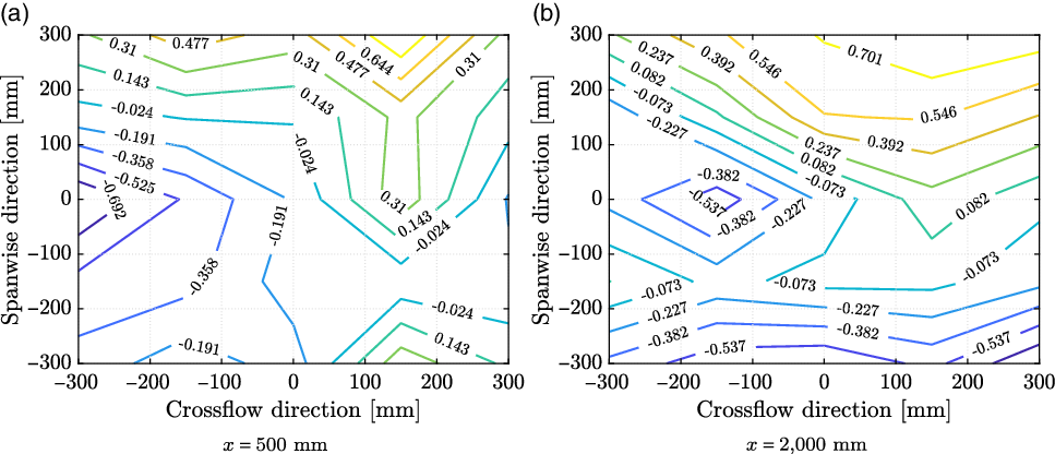
Figure 8. Flow speed non-uniformity levels at 15 m/s measured at scanning plans located 500 and 2,000 mm from the test section entrance.
HWA measurements were taken along the tunnel centreline in the streamwise direction at every 150 mm between 500 and 2,000 mm from the test section entrance, for 15 and 25 m/s, Fig. 9. The results show the difference with respect to the mean; the variation is within
 $\pm$
1%. The wall divergence was able to partially compensate for the boundary layer growth on the wall. The variation was higher for the lower speeds, which is consistent with the boundary layer being thicker at lower speeds.
$\pm$
1%. The wall divergence was able to partially compensate for the boundary layer growth on the wall. The variation was higher for the lower speeds, which is consistent with the boundary layer being thicker at lower speeds.
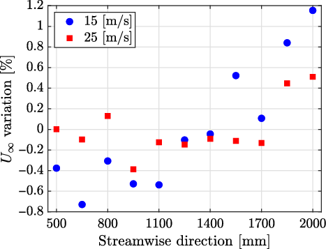
Figure 9. Flow speed variation along the test section centreline.

Figure 10. Wind-tunnel background noise spectra measured with a microphone, coupled with a nose cone, positioned in the airflow.
3.4 Acoustic background noise
Numerous studies have been published for research [Reference Mathew, Bahr, Sheplak, Carroll and Cattafesta13, Reference Mayer, Kamliya, Szöoke, Ali and Azarpeyvand23, Reference Liu, Xing, Guo and Li44, Reference Leclercq, Doolan and Reichl82–Reference Vathylakis, Chong and Kim87] and industrial [Reference Wickern and Lindener88–Reference Duell, Yen, Arnette and Walter91] open-jet wind tunnels about background acoustic noise level characterisation. However, for closed-section wind tunnels the literature is scarce and within the authors’ knowledge, there is no established methodology.
In our measurements, the instrumentation employed to characterise the wind-tunnel acoustic background noise includes a G.R.A.S. Sound & Vibration 46BD pre-amplified microphone coupled with a G.R.A.S. Sound & Vibration RA0022 nose cone. With the aid of the traverse system, the microphone was positioned in the test section centreline, 0.5 m distant from the test section entrance. The microphone operates in the 4 Hz to 70 kHz frequency range with
 $\pm$
2 dB accuracy. Its upper limit of dynamic range is 166 dB and its sensitivity is approximately 1.45 mV/Pa. Data was acquired with the National Instruments system described in Section 3.1.
$\pm$
2 dB accuracy. Its upper limit of dynamic range is 166 dB and its sensitivity is approximately 1.45 mV/Pa. Data was acquired with the National Instruments system described in Section 3.1.
Acoustic data were acquired at 48 kHz sample rate during 20 s. For the calculation of the sound power spectrum, the time series was segmented into data blocks with 50% data overlap prior to the application of a Hanning windowing function over each block. In performing the Fourier Transform a correction factor associated with the windowing function energy loss [Reference Bendat and Piersol92] was applied. Averaging over all block spectra provided the mean noise spectrum, which was evaluated in terms of Power Spectral Density (PSD), with 1 Hz resolution.
Figure 10 displays the wind-tunnel background noise for several flow speeds. Figure 10(a) also includes the noise measured by a microphone in test section with no flow, but with the fan-motor controller already energised. For speeds 15 m/s and above, the noise of the in-flow microphone is substantially higher than this noise floor. The spectra, Fig. 10(a), show that noise level increases with the flow speed. Mach number scaling to the fifth power is exhibited in Fig. 10(b), where a collapse for frequencies lower than 3 kHz is observed. Results in Strouhal number, based on the freestream speed and test section characteristic length of 1 m are shown in Fig. 10(c). Mach to the fourth power provided a reasonable collapse for Strouhal numbers higher than 20. This observation suggests that the lower and the higher frequency noise have different nature, but we made no attempt at identifying them. No narrow band peaks that could be associated with the fan blade passing frequency were observed.
The Overall Sound Pressure Level (OASPL) was evaluated between 1 and 10,000 Hz frequency range for several flow speeds and the results are shown in Fig. 11. Regarding flow speed scaling, a good fit was obtained for the 4th power of Mach number. This is lower than the power law obtained for the spectra in Fig. 10. The fifth power is adequate for most of the spectra, i.e. frequencies above 50 Hz. Below this frequency, which is the dominant part of the spectra, this power provides an over correction, which explains the 4th power obtained for the OASPL. Data from the KSWT (2), obtained in the same frequency range are also displayed. Both facilities show a similar background noise level, although the KSWT (2) is approximately 2.5 dB quieter than the LANT for lower flow speeds. Both wind-tunnels are closed-loop and closed-section, but the KSWT (2) has a test section 1.4 m in height
 $\times$
1.4 m in width
$\times$
1.4 m in width
 $\times$
4.9 m in length, whereas the LANT test section is 1-m high
$\times$
4.9 m in length, whereas the LANT test section is 1-m high
 $\times$
1-m wide
$\times$
1-m wide
 $\times$
3-m long. For the KSWT (2) measurements were taken at approximately 2.05 m downstream of the test section entrance at the tunnel centreline. We do not know what impact these differences could have on the measured noise, but we were satisfied that LANT wind tunnel met the set target. A-weighted OASPL values evaluated between 1 and 10,000 Hz frequency range are also given in the figure. OASPL values based on the more conventional frequency range of 100–10,000 Hz are given in the figure together with A-weighted OASPL for this frequency range. These values are much lower. Results are still difficult to compare with other wind tunnels because no standard procedure is established for such measurements. It nevertheless seems that our noise level is about 10 dBA higher than that of anechoic chamber facilities and similar to that of a larger closed-section wind tunnel.
$\times$
3-m long. For the KSWT (2) measurements were taken at approximately 2.05 m downstream of the test section entrance at the tunnel centreline. We do not know what impact these differences could have on the measured noise, but we were satisfied that LANT wind tunnel met the set target. A-weighted OASPL values evaluated between 1 and 10,000 Hz frequency range are also given in the figure. OASPL values based on the more conventional frequency range of 100–10,000 Hz are given in the figure together with A-weighted OASPL for this frequency range. These values are much lower. Results are still difficult to compare with other wind tunnels because no standard procedure is established for such measurements. It nevertheless seems that our noise level is about 10 dBA higher than that of anechoic chamber facilities and similar to that of a larger closed-section wind tunnel.

Figure 11. Wind-tunnel background noise OASPL. KSWT (2) data extracted from [Reference Hunt, Downs, Kuester, White and Saric9].
The traverse used to place the microphone in the flow may be a source of noise and we did our best to reduce noise produced from it by, for example, fairing and prevention of vibration. Our judgment is that the contribution of the traverse is not the dominant one, because different arrangements of in-flow microphone measurements led to the same result. A complementary study on the LANT background acoustic noise is given by Serrano et al. [Reference Serrano, Amaral, Bresci and Medeiros93]. There, the noise was measured with a microphone array and beamforming techniques instead of a microphone placed in the airflow, in a procedure similar to the one described in Section 4.2. Using beamforming, the result depends crucially on the parameters used, particularly the Region of Integration (ROI) [Reference Brooks and Humphreys94]. We chose to present here results of the in-flow microphone to allow comparison with other wind tunnels. However, if the study will use beamforming, which is the most common procedure for closed-section wind tunnels, the most relevant background noise level would be provided by this technique.
4.0 Benchmark experiments
4.1 Laminar boundary layer over a flat-plate
As a benchmark experiment in flow stability, we investigated a two-dimensional laminar and transitional flat plate boundary layer. Figure 12 exhibits a sketch of the flat plate model employed. The model consists of four elements: (1) an 120 mm long leading-edge of 10 mm thickness, (2) a plexiglass flat plate 1.8-m long and 10-mm thick, (3) a flap and (4) a tab, with a combined 200 mm chord. Its leading edge was an asymmetric 2:1 aspect ratio super-ellipse, aiming at better controlling the model suction peak and improving the quality of the zero-pressure gradient on the model working side [Reference Hanson, Buckley and Lavoie95]. The super-ellipse derivatives along the chord axis smoothly approaches zero, which prevents a discontinuity at the junction between the leading-edge (1) and the main element (2). The flap was used to adjust the pressure gradient on the model surface and the tab controlled the stagnation point. To monitor the chordwise pressure gradient, 30 pressure taps were distributed along a line distant 250 mm from the model mid-span. Such taps were connected to a multi-tube manometer. The model was vertically installed at the centreline of the tunnel test section spanning the whole section height.

Figure 12. Diagram of the flat plate model employed for the boundary layer experiments. Dimensions in millimetres. The model super-ellipse leading edge is shown in detail.
HWA measurements of the mean velocity were performed at two different streamwise stations, located 200 and 900 mm from the model leading-edge. For each of the two streamwise positions, the velocity profile was mapped along the wall-normal direction (y direction) with steps of 0.10 and 0.20 mm, respectively. The experiment covered the spanwise range of
 $\pm$
150 and
$\pm$
150 and
 $\pm$
240 mm for the 200 and 900 mm streamwise stations, respectively, with a discretisation of 30 mm. The freestream velocity was set at 16.5 m/s. Under these conditions, the boundary layer was very thin (
$\pm$
240 mm for the 200 and 900 mm streamwise stations, respectively, with a discretisation of 30 mm. The freestream velocity was set at 16.5 m/s. Under these conditions, the boundary layer was very thin (
 $\delta^*$
approximately 0.8 mm) and it was very difficult to measure the distance from the probe to the wall. As is common in flat plate laminar boundary layer experiments, this distance was obtained based on the velocity profile measured [Reference Paula, Würz, Mendonça and Medeiros96]. The freestream velocity was calculated as the mean of the 5 points measured outside the boundary layer. Using this speed and the distance from the leading edge a theoretical Blasius profile was calculated and the distance from the wall was obtained by visually matching the measured and theoretical profiles.
$\delta^*$
approximately 0.8 mm) and it was very difficult to measure the distance from the probe to the wall. As is common in flat plate laminar boundary layer experiments, this distance was obtained based on the velocity profile measured [Reference Paula, Würz, Mendonça and Medeiros96]. The freestream velocity was calculated as the mean of the 5 points measured outside the boundary layer. Using this speed and the distance from the leading edge a theoretical Blasius profile was calculated and the distance from the wall was obtained by visually matching the measured and theoretical profiles.
Figure 13 displays a good comparison between the experimental results and the theoretical Blasius profile, also lending support to the procedure for establishing the distance from the wall.

Figure 13. Comparison between experimental and Blasius boundary layer profiles for two streamwise stations.

Figure 14. Comparison of boundary layer velocity profiles from the current experiment (continuous lines) and that of Medeiros and Gaster(1999) [Reference Medeiros and Gaster97] (dashed lines).
The results were compared with those obtained by Medeiros and Gaster [Reference Medeiros and Gaster97] in the Gaster’s wind tunnel (15) in Figure 22. The experiments were not at identical Reynolds numbers, but are comparable. Their freestream velocity was 17.3 m/s. The first measurement station from Medeiros and Gaster [Reference Medeiros and Gaster97] was 300 mm from the leading-edge (
 $Re_{\delta^*} = 915$
, i.e. Reynolds number based on the displacement thickness
$Re_{\delta^*} = 915$
, i.e. Reynolds number based on the displacement thickness
 $\delta^*$
), whereas for our experiment it was 200 mm (
$\delta^*$
), whereas for our experiment it was 200 mm (
 $Re_{\delta^*} = 738$
). For the second measurement station, both data were obtained at a streamwise station 900 mm from the leading-edge, although for our experiment,
$Re_{\delta^*} = 738$
). For the second measurement station, both data were obtained at a streamwise station 900 mm from the leading-edge, although for our experiment,
 $Re_{\delta^*} = 1,620$
, and for Medeiros and Gaster [Reference Medeiros and Gaster97] experiment,
$Re_{\delta^*} = 1,620$
, and for Medeiros and Gaster [Reference Medeiros and Gaster97] experiment,
 $Re_{\delta^*} = 1,593$
. In Figure 22, the solid lines represent the current experiments, whereas the dashed lines represent the results from Medeiros and Gaster [Reference Medeiros and Gaster97]. One figure represents the initial stage of the boundary layer and the other, a later stage. At both streamwise stations, the LANT wind tunnel, presents a more two-dimensional flow, particularly close to surface, which is the region with higher impact on Tollmien-Schlichting (TS) wave growth.
$Re_{\delta^*} = 1,593$
. In Figure 22, the solid lines represent the current experiments, whereas the dashed lines represent the results from Medeiros and Gaster [Reference Medeiros and Gaster97]. One figure represents the initial stage of the boundary layer and the other, a later stage. At both streamwise stations, the LANT wind tunnel, presents a more two-dimensional flow, particularly close to surface, which is the region with higher impact on Tollmien-Schlichting (TS) wave growth.
Natural boundary layer transition over the flat plate model was also verified. The shape factor H, defined as the ratio between the displacement (
 $\delta^{*}$
) and the momentum (
$\delta^{*}$
) and the momentum (
 $\theta$
) thicknesses, is often used to indicate transition. According to Schubauer and Klebanoff [Reference Schubauer and Klebanoff98], a strong reduction in the shape factor H (
$\theta$
) thicknesses, is often used to indicate transition. According to Schubauer and Klebanoff [Reference Schubauer and Klebanoff98], a strong reduction in the shape factor H (
 $\delta^{*}/\theta$
) is observed at the transition region, decreasing from a value of 2.59 in the laminar region (in a flat plate experiment) to approximately 1.4 in the turbulent region. Boundary layer flow profiles were obtained at several chordwise positions, between 50 and 1,900 mm from the model leading-edge, and freestream speeds between 10 and 25 m/s. Figure 14 summarises the results and indicates that transition, which initiated at approximately
$\delta^{*}/\theta$
) is observed at the transition region, decreasing from a value of 2.59 in the laminar region (in a flat plate experiment) to approximately 1.4 in the turbulent region. Boundary layer flow profiles were obtained at several chordwise positions, between 50 and 1,900 mm from the model leading-edge, and freestream speeds between 10 and 25 m/s. Figure 14 summarises the results and indicates that transition, which initiated at approximately
 $Re_x \approx 2.5 \times 10^6$
, was not completed on the plate at these speeds.
$Re_x \approx 2.5 \times 10^6$
, was not completed on the plate at these speeds.

Figure 15. Flat plate model boundary layer shape factor (H) as a function of Reynolds number (
 $Re_x$
).
$Re_x$
).
Figure 15 exhibits the natural boundary-layer transition limits in terms of
 $Re_x$
number
$Re_x$
number
 $\left(= \frac{U_{\infty}x}{\nu}\right)$
and freestream turbulence
$\left(= \frac{U_{\infty}x}{\nu}\right)$
and freestream turbulence
 $\left(\frac{100\sqrt{\frac{1}{3}(u_{\rm rms}^2 + v_{\rm rms}^2 + w_{\rm rms}^2})}{U_{\infty}}\right)$
, established by Schubauer and Skramstad [Reference Schubauer and Skramstad99]. In this figure, the markers indicate the values obtained experimentally by Schubauer and Skramstad [Reference Schubauer and Skramstad99] for the transition as a function of the stream turbulence fit by the solid lines. The horizontal dash-dotted line indicates the initial transition Reynolds number in our experiment. The picture suggests our background turbulence level based on the mean of all three velocity components would be about 0.14%, which is not consistent with our measurements of
$\left(\frac{100\sqrt{\frac{1}{3}(u_{\rm rms}^2 + v_{\rm rms}^2 + w_{\rm rms}^2})}{U_{\infty}}\right)$
, established by Schubauer and Skramstad [Reference Schubauer and Skramstad99]. In this figure, the markers indicate the values obtained experimentally by Schubauer and Skramstad [Reference Schubauer and Skramstad99] for the transition as a function of the stream turbulence fit by the solid lines. The horizontal dash-dotted line indicates the initial transition Reynolds number in our experiment. The picture suggests our background turbulence level based on the mean of all three velocity components would be about 0.14%, which is not consistent with our measurements of
 $Tu < 0.1\%$
. It must be taken into account that Schubauer and Skramstad [Reference Schubauer and Skramstad99] established transition using a Preston tube, while our approach was different. It is also not clear what was the frequency band used in their experiment. In view of these uncertainties, we are satisfied that our results are close to theirs. The initial transition location in our experiment, (
$Tu < 0.1\%$
. It must be taken into account that Schubauer and Skramstad [Reference Schubauer and Skramstad99] established transition using a Preston tube, while our approach was different. It is also not clear what was the frequency band used in their experiment. In view of these uncertainties, we are satisfied that our results are close to theirs. The initial transition location in our experiment, (
 $Re_x \approx 2.5 \times 10^6$
) was close to the limit indicated in Fig. 16. According to the same figure, the transition ends at
$Re_x \approx 2.5 \times 10^6$
) was close to the limit indicated in Fig. 16. According to the same figure, the transition ends at
 $Re_x \approx 3.9 \times 10^6$
, which is the limit.
$Re_x \approx 3.9 \times 10^6$
, which is the limit.

Figure 16. Natural boundary layer transition limit Schubauer and Skramstad [Reference Schubauer and Skramstad99]. The dash-dotted line indicates the values obtained experimentally.
Figure 16 exhibits the PSD of the HWA signals at
 $x = 900$
mm and
$x = 900$
mm and
 $\eta \approx 1$
, which corresponds to the TS wave inner peak location. For the calculation of this spectrum, an 11 s long time series was collected at a sampling rate of 25 kHz. The signal was divided into 66 data blocks, and a Hanning window was applied to each block with no overlap. The Fourier transform was taken and averaged over the blocks.
$\eta \approx 1$
, which corresponds to the TS wave inner peak location. For the calculation of this spectrum, an 11 s long time series was collected at a sampling rate of 25 kHz. The signal was divided into 66 data blocks, and a Hanning window was applied to each block with no overlap. The Fourier transform was taken and averaged over the blocks.

Figure 17. TS peak PSD obtained at the position
 $z = -30$
mm and
$z = -30$
mm and
 $\eta \approx 1$
.
$\eta \approx 1$
.
Figure 17 shows the amplification of the two-dimensional instability waves as computed by the integration of the growth rates obtained from the Orr-Sommerfeld Equation (OSE) starting from the first branch of each wave. To facilitate comparison, the experimental and numerical results are normalised by their spectral peak. The agreement is good. It is recognised that in natural transition there will be a certain amount of oblique waves which would tend to display lower frequencies. Nevertheless, the 2D wave is expected to be the dominant and this procedure is often presented used in the literature [Reference Crouch, Kosorygin and Sutanto100, Reference Crouch and Kosorygin101].

Figure 18. Comparison between OSE and the experiment.
To obtain an experimental estimate of the TS wave amplitude distribution the following procedure was adopted. The integral of the PSD in the frequency range 156–180 Hz was obtained for the signal at different distances from the wall. Figure 18 shows the comparison between theoretical and experimental TS amplitude distribution, represented by the solid line and markers, respectively. The agreement is good.

Figure 19. Comparison between numerical (continuous lines) and experimental (markers) normalised TS profiles.
4.2 Acoustic radiation from an immersed cylinder
The benchmark test chosen for wind tunnel validation in aeroacoustics was the sound from a cylinder immersed in a flow, an experiment employed for several aeroacoustic facilities [Reference Mayer, Kamliya, Szöoke, Ali and Azarpeyvand23, Reference Leclercq, Doolan and Reichl82, Reference Vathylakis, Chong and Kim87]. A cylindrical wire of
 $1.3$
mm diameter was clamped to the test section floor and ceiling. Experiments were performed in the 13.1–25.4 m/s flow speed range. For this study, measurements were conducted with the antenna specially designed for the LANT facility. The tunnel working section can be considered small for beamforming experiments. Limited aperture of microphone arrays can lead to poor beamforming resolution at low frequency [Reference Mueller102]. This however was mitigated with an optimised array design [Reference Amaral, Serrano and Medeiros103]. The microphones distribution play an important role in the array performance. Optimising the microphones distribution is fundamental for obtaining good resolution without loss of dynamic range.
$1.3$
mm diameter was clamped to the test section floor and ceiling. Experiments were performed in the 13.1–25.4 m/s flow speed range. For this study, measurements were conducted with the antenna specially designed for the LANT facility. The tunnel working section can be considered small for beamforming experiments. Limited aperture of microphone arrays can lead to poor beamforming resolution at low frequency [Reference Mueller102]. This however was mitigated with an optimised array design [Reference Amaral, Serrano and Medeiros103]. The microphones distribution play an important role in the array performance. Optimising the microphones distribution is fundamental for obtaining good resolution without loss of dynamic range.
The antenna is populated with 112 1/4-in G.R.A.S. Sound & Vibration 40PH microphones. Such microphones have a frequency range reaching up to 20 kHz, a dynamic range topping at approximately 135 dB, an accuracy of
 $\pm$
2 dB, up to 20 kHz, and a sensitivity of approximately 50 mV/Pa. In-house conventional beamforming algorithms [Reference Amaral and Pagani60, Reference Pagani, Caldas and Medeiros104] were employed to post-process the microphone array data. Such algorithms [Reference Mueller102, Reference Chiariotti, Martarelli and Castellini105, Reference Merino-Martínez, Sijtsma, Snellen, Ahlefeldt, Antoni, Bahr, Blacodon, Ernst, Finez, Funke, Geyer, Haxter, Herold, Huang, Humphreys, Leclère, Malgoezar, Michel, Padois, Pereira, Picard, Sarradj, Siller, Simons and Spehr106] steer the microphone array to a chosen region and estimate the acoustic noise source magnitude and distribution in the region.
$\pm$
2 dB, up to 20 kHz, and a sensitivity of approximately 50 mV/Pa. In-house conventional beamforming algorithms [Reference Amaral and Pagani60, Reference Pagani, Caldas and Medeiros104] were employed to post-process the microphone array data. Such algorithms [Reference Mueller102, Reference Chiariotti, Martarelli and Castellini105, Reference Merino-Martínez, Sijtsma, Snellen, Ahlefeldt, Antoni, Bahr, Blacodon, Ernst, Finez, Funke, Geyer, Haxter, Herold, Huang, Humphreys, Leclère, Malgoezar, Michel, Padois, Pereira, Picard, Sarradj, Siller, Simons and Spehr106] steer the microphone array to a chosen region and estimate the acoustic noise source magnitude and distribution in the region.
Figure 19 exhibits a sketch containing the cylindrical wire (thick continuous line), the test section top and bottom walls (narrow continuous line) and the array microphones (blue filled circles). The mesh (dashed-dotted lines) is 1,250 mm long in the spanwise direction and 2,500 mm long in the streamwise direction, 460 mm distant from the microphone array where the wire was placed. The resolution reduces if the source is not located in the array focus [Reference Amaral, Serrano and Medeiros103]. Hence, this constitutes a more demanding test. A Region of Integration (ROI) is defined as a subspace of the mesh (dashed lines in Fig. 20), in our case, measuring 750 and 200 mm in spanwise and streamwise directions, respectively, centred at the wire position. The ROI is employed to estimate the spectra of the noise emitted by the wire.

Figure 20. Sketch containing the cylindrical wire (thick continuous line), test section top and bottom walls (thin continuous lines), array microphones (blue filled circles), mesh (dash-dotted lines) and ROI (dashed lines). The freestream speed is from left to right.
For each beamforming evaluation, microphone data were acquired at 48 kHz during 20 s. The Cross-Spectral Matrix (CSM) of the sound pressure measurements of the array microphones was calculated through the segmentation of the time series into data blocks of 50% overlap and application of a Hanning windowing on each block. The outer product of the Fourier Transformed data blocks of pairs of microphones was calculated and averaged over all blocks. Correction factors owing to the windowing function energy loss [Reference Bendat and Piersol92] and location of the microphones on a hard wall [Reference Fischer and Doolan38] were applied. Further details of the procedure used can be obtained in Amaral et al. [Reference Amaral and Pagani60]. The CSM diagonal was discarded for the reduction of noise contamination associated with the wind-tunnel wall boundary layer turbulence on the microphones [Reference Mueller102].
Figure 20 exhibits the resulting noise spectra. There were narrow band peaks whose frequency increased with the freestream speeds. The spectra collapsed on a non-dimensional scaling of Strouhal number based on the cylindrical wire diameter and the freestream speed. The peak at Strouhal number of 0.21 agrees very well with literature [Reference Blake107].

Figure 21. Cylinder noise spectra measured with the microphone phased array and post-processed with in-house conventional beamforming algorithm.
Conventional beamforming acoustic source maps are displayed in Fig. 22, obtained at freestream speeds of 17.5 and 21.9 m/s, for 2.85 and 3.6 kHz frequencies, respectively, both corresponding to Strouhal number 0.21. The acoustic source is well defined and mapped along the cylindrical wire span. The noise source was better represented for the higher frequency, consistent with the fact that the beamforming resolution increases with frequency [Reference Mueller102]. The quality of the beamforming results, regarding the resolution of the acoustic maps and the levels of the noise spectra, can be enhanced if, among other practices, deconvolution algorithms and array shading are employed [Reference Amaral and Pagani60], and a test section foamed-walls set-up is available [Reference Amaral and Pagani60]. We refrained from using these techniques to offer a more transparent and accessible measure of the wind tunnel quality.
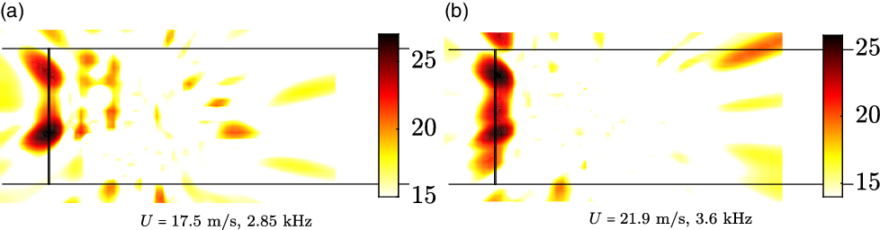
Figure 22. Conventional beamforming acoustic source maps for the cylindrical wire experiments for
 $St = 0.21$
. The different freestream speeds were from left to right.
$St = 0.21$
. The different freestream speeds were from left to right.
5.0 Conclusions
The design, construction and flow quality assessment of the LANT wind tunnel is reported in this paper. The tunnel is of the closed-loop and closed test section type and is designed for low turbulence and low acoustic background noise. The fan is composed of a 16-blade rotor and 13-blade stator. Currently the top speed is 30 m/s, but there is provision to double the speed. At the corners, the wind tunnel walls are covered with acoustic absorbent material and possess turning vanes filled with acoustic absorbent material. The tunnel circuit presents several narrow angle diffusers and, just upstream of the settling chamber, one wide angle diffuser, where boundary layer separation is prevented by a screen. The settling chamber features five screens (mesh 0.95 mm) and a honeycomb (cell diameter 3.175 mm). Downstream of the last screen a long empty settling chamber was left for residual turbulence decay. The 7:1 area ratio contraction was short to reduced working section wall boundary layer thickness and designed by the hodograph method.
HWA measurements indicate freestream turbulence level between 0.050% and 0.071% in the range of freestream velocities of 10 and 30 m/s. Such value was obtained employing the commonly used dynamic filter that selects the cutoff frequency based on the tunnel freestream speed and test-section dimensions [Reference Lindgren and Johansson21]. The high-pass filter frequency cutoff were 5, 7.5, 10, 12.5 and 15 Hz for 10, 15, 20, 25 and 30 m/s freestream speeds, respectively. A low-pass filter of 10 kHz was also used [Reference Hunt, Downs, Kuester, White and Saric9]. This level of turbulence is close to that of MTL wind tunnel (10), a well-known reference wind tunnel which used the same kind of filter.
The freestream turbulence spectra are similar to that of the KSWT (2), another recognised facility for transition studies, in the frequency range 1 Hz to 10 kHz, but higher than that of the Gaster’s wind tunnel (15) which is remarkably low.
The test section wall boundary layers were measured, including the turbulence intensity. It was found that the freestream turbulence levels discussed above are observed in the 800
 $\times$
800 mm
$\times$
800 mm
 $^2$
central region of the test section. We could not find this figure in the extensive literature we covered, but from personal communications, it appeared that maintaining the wind tunnel wall boundary layer and turbulence within 10 cm in a 3 m long working section with a long settling chamber is a very good result. At a speed of 15 m/s, the flow in the test section central region was uniform within roughly 1%, a level similar to that of the KSWT (2).
$^2$
central region of the test section. We could not find this figure in the extensive literature we covered, but from personal communications, it appeared that maintaining the wind tunnel wall boundary layer and turbulence within 10 cm in a 3 m long working section with a long settling chamber is a very good result. At a speed of 15 m/s, the flow in the test section central region was uniform within roughly 1%, a level similar to that of the KSWT (2).
The OASPL acoustic background noise evaluated in the 1–10,000 Hz frequency range is approximately 90 and 110 dB at freestream speeds of 10 and 30 m/s, respectively. This is similar to the noise levels reported for the KSWT (2). In summary, the design targets, namely, turbulence intensity level below 0.1%, uniformity within 1% and acoustic background noise below 110 dB at 30 m/s in a useful area of
 $800 \times 800$
mm
$800 \times 800$
mm
 $^2$
were achieved.
$^2$
were achieved.
A laminar and transitional flat plate boundary layer was also carried out as a benchmark for instability experiments. A boundary layer profile with almost perfect agreement with Blasius theory was measured at a
 $Re_{\delta^*} = 738$
and 1620, corresponding to distances of 200 and 900 mm from the leading edge, respectively. It was also shown the boundary layer was two-dimensional to a degree higher than that reported in studies of Gaster’s wind tunnel (15). Natural transition initiated at
$Re_{\delta^*} = 738$
and 1620, corresponding to distances of 200 and 900 mm from the leading edge, respectively. It was also shown the boundary layer was two-dimensional to a degree higher than that reported in studies of Gaster’s wind tunnel (15). Natural transition initiated at
 $Re_x \approx 2.5 \times 10^6$
. This is close to the limit of laminar flow as established by Schubauer and Skramstad [Reference Schubauer and Skramstad99]. Indeed, at 25 m/s transition was not completed on the model. The streamwise velocity spectral content and amplitude distribution inside the boundary layer prior to transition were agreed with predictions of linear stability theory for TS waves.
$Re_x \approx 2.5 \times 10^6$
. This is close to the limit of laminar flow as established by Schubauer and Skramstad [Reference Schubauer and Skramstad99]. Indeed, at 25 m/s transition was not completed on the model. The streamwise velocity spectral content and amplitude distribution inside the boundary layer prior to transition were agreed with predictions of linear stability theory for TS waves.
A benchmark experiment on aeroacoustics was also carried out, namely, the noise emitted from a cylinder immersed in the flow. A 1.3 mm wire was used as the cylinder. A microphone phased array acquired the acoustic signals and an in-house conventional beamforming algorithm post-processed the data to generate the acoustic maps and evaluate the noise spectra. The experiment successfully captured the sound emitted from the wire. For a range of freestream speeds, a spectral narrowband peak was observed and corresponded to a Strouhal number of 0.21, the value established in the literature. At this Strouhal number, a well-defined acoustic source was mapped at the wire position.
The wind tunnel can be considered small for beamforming studies, but the results show that, which an optimised array design, is capable of housing such studies. In general, the design was not innovative, as it mostly used strategies already established in the design of other tunnels. However, it is innovative in the sense that it combined in a single tunnel, different strategies used in different tunnels. It is also innovative in that it was designed from the start for stability and aeroacoustic experiments, where, in general, tunnels have been adapted for aeroacoustic used after being built. Another important innovative aspect was that it used a very long stretch of settling chamber after the last screen which is often thought to increase boundary layer thickness on the test section wall, reducing flow quality and useful area. The results showed that, in combination with short contraction the thickness of these boundary layer is controlled. The overall conclusion is that the wind tunnel described is well suited for its design purpose, namely, stability experiments, in particular boundary layer transition, and aeroacoustics experiments.
Acknowledgments
F.R.A. received funding from Coordination for the Improvement of Higher Education Personnel (CAPES/Brazil), grant #DS00011/07-0, and from Sao Paulo Research Foundation (FAPESP/Brazil), grant #2019/02203-2. J.C.S.R. received support from National Council for Scientific and Technological Development (CNPq/Brazil), grant #140211/2014-4, and from University of Pamplona. C.S.B. was supported by CAPES/Brazil, grant #88882.379171/2019-1. M.M.B. was funded by CAPES/Brazil, grant #88882.379172/2019-1. V.B.V. received support from CNPq/Brazil, grant #134335/2018-0. E.M.G, J.C.S.R. and M.A.F.M received funding from CNPq/Brazil, grant #381443/2012-4. M.A.F.M. was funded from CNPq/Brazil, grant #307956/2019-9, and from the Air Force Office of Scientific Research (AFOSR/USA), grant #FA9550-18-1-0112, managed by Dr. Geoff Andersen from Southern Office of Aerospace Research and Development (SOARD). The project financial support was provided by Funding Authority for Studies and Projects (FINEP/Brazil), grant #01.09.0334.04, and from FAPESP/Brazil, grants #2006/52568-7 (in the context of the Brazilian Silent Aircraft Program) and #2019/15366-7. The authors are also indebted to Fernando Henrique Tadashi Himeno, Marlon Sproesser Mathias, Fabio Luis Gallo, José Cláudio Pinto de Azevedo, Hernan Dario Ceron Muñoz, Leandro Guilherme Crenite Simões, Fernando Martini Catalano and many others who somehow contributed to this project.


