NOMENCLATURE
- AOA
-
angle-of-attack
- BVI
-
blade vortex interaction
- C
-
blade chord length
- Cn
-
radial force coefficient of blade 1 in moving frame, in terms of the blade tangential velocity
- Ct
-
tangential force coefficient of blade 1 in moving frame, in terms of the blade tangential velocity
- FM
-
figure of merit
- LESB
-
leading-edge separation bubble
- LEV
-
leading-edge vortex
- MAV
-
micro-aerial vehicle
- P
-
power consumed by cycloidal propeller
- PL
-
power loading
- Q
-
torque caused by cycloidal propeller
- S
-
area of the blade
- T
-
thrust of the cycloidal propeller, it is the resultant force of vertical force and side force
- Tc
-
time of one cycle
- TEV
-
trailing-edge vortex
- V
-
tangential velocity of the blade observed in the inertial frame
- Vy
-
vertical velocity of the air observed in the inertial frame
- αp
-
blade pitch angle
- θ
-
azimuth angle of the cycloidal propeller
- ρ
-
air density
- ω
-
rotation speed of the cycloidal rotor in inertial frame. ω > 0 when cycloidal rotor rotates in counter-clock-wise direction
- ωbi
-
pitch rate of blade i in moving frame. ωbi > 0 when blade i pitches in counter-clockwise direction
1.0 INTRODUCTION
Cyclogyro or cyclocopter is a type of rotorcraft which flies by cycloidal propellers. The cycloidal propeller is a kind of rotor whose blades rotate around an axis parallel to the rotor shaft. The blade control is varied cyclically along an azimuth in each revolution by a control ring that is located eccentrically to the rotor shaft. The motion of each blade is comprised of the rotation about the rotor axis and the pitching oscillation about its pitching axis. If viewed in the moving reference frame attached to the cycloidal propeller, each blade is actually performing a pitch oscillation in the curvilinear flow. If the position of the control ring varied, the magnitude and the direction of the thrust will be instantly changed. Therefore, the cycloidal propeller can provide instant omni-directional vectored thrust. This provides the cyclogyro with very good manoeuvrability. This is very useful for the Micro-Aerial Vehicles (MAVs) that fly in closed space and indoors.
The cyclogyro has been studied since the early 20th century. However, only within the recent decade, there were major progresses for cyclogyro. Gil Iosilevskii and Yuval Levy performed both experiments and Computational Fluid Dynamics (CFD) simulations with a small cycloidal propeller with the diameter of 0.11m(Reference Iosilevskii and Levy1,Reference Iosilevskii and Levy2) . The results of Fast Fourier Transformation on the vertical force coefficients indicated that there are strong interactions between the blades and the wakes of neighbouring blades(Reference Iosilevskii and Levy1). The numerical simulation results also indicated that the cycloidal propeller can be compared with heavy-loaded helicopter rotor. Seong Hwang et al. developed a quad-rotor cyclogyro and proved that the cycloidal propeller can provide enough thrust for hovering and forward flight(Reference Kim, Yun and Kim3−Reference Hwang, Min and Lee8). Benedict et al conducted extensive experimental and numerical simulations on the cycloidal propellers for MAVs(Reference Benedict, Chopra, Ramasamy and Leishman9,Reference Yang14) . According to their experiments and analyses, they concluded that, compared to a conventional rotor, each span-wise blade element of a cyclorotor operates at similar aerodynamic conditions, so the blades can be more easily optimised to achieve the best aerodynamic efficiency, and the cycloidal rotors are more efficient at low Reynolds numbers because of the unsteady aerodynamic effects associated with cycloidal blades(12). The aero-elastic analysis also showed that the low-torsion flexibility of the blade will cause lower thrust of the cycloidal propeller(11). They also developed a cyclogyro which can fly in any direction(Reference Benedict, Gupta and Chopra13). Kan Yang made a CFD analysis incorporated with the structural model developed by Moble Benedict. The CFD analysis was conducted, based on a small-scale cycloidal rotor for MAV with a radius of 70.6mm and a blade span of 141.1mm(Reference Yang14). The CFD simulation results showed that the simulation based on a 2D mesh system corresponds to the mid-span section of the 3D mesh system. Both the 2D and 3D simulation can obtain a fairly good prediction on the vertical force, but cannot capture side force well and under-predicts the power. Both 2D and 3D simulations can obtain fairly good flow fields, if compared with results from Particle Image Velocimetry (PIV). Therefore, the results from the CFD simulation was used to qualitatively explore the characteristics of the flow field(Reference Yang14).
A series of experiments on the cycloidal propellers for the MAVs were conducted by us, as well. Based on these experiments, two cyclogyroes were developed. The first one was equipped with two contra-rotating cycloidal propellers and two screw propellers. Its span is 1,300mm and it weighted 1.35kg. The second one was equipped with two cycloidal propellers rotating in the same direction and a tail rotor to provide both yaw and pitch control. Its span was 700mm and it weighted 1.1kg. This cyclogyro can be precisely controlled and can stay in the air for more than 5min with 300g of payload. All these cyclogyroes were flying by cycloidal propellers with 2mm plate aerofoils.
From previous research work, it can be seen that the unsteady aerodynamic effects associated with cycloidal blades have a significant impact on the aerodynamic forces of the cycloidal rotor. However, although extensive experimental and simulation results were obtained by previous research work, the mechanism behind the high efficiency of cycloidal propellers is yet to be understood.
To improve the understanding of the cycloidal propeller, the unsteady aerodynamic effects of the blade dynamic stall, parallel Blade Vortex Interaction (BVI), inflow variation and flow curvature were discussed in this paper. The 2D CFD simulations were performed on the cycloidal propeller with a flat plate aerofoil in hovering status and compared with the results of the experiment. Then, the streamlines and vorticity contours were drawn in the moving frame. This helped us to better understand the flow structure around and within the cycloidal propeller. Finally, the unsteady aerodynamic effects mentioned above will be discussed based on the results from numerical simulations.
2.0 THE EXPERIMENT APPARATUS
As shown in Fig. 1, the experiment apparatus consists of a six-component force balance developed by China Aerodynamics Research and Development Center (CARDC), the data acquisition and conditioning system, a high-precision excitation power source and a cycloidal propeller driven by a Panasonic servo motor. The ranges of the components on vertical force and horizontal force are 150N and 50N, respectively. The range of the torque is 5nm. In order to avoid large impulsive forces produced by cycloidal rotor damage from the force balance and also to sustain the weight of the cycloidal rotor system, the range of the force balance is relatively large in comparison with the mean aerodynamic forces of the cycloidal rotor. However, the force balance has been carefully designed and systematically calibrated, such that the maximum relative static error of each force component is less than 0.3%. A high-precision power supply was used to provide 12V excitation voltage with maximum error of 5μV. The data acquisition and conditioning system is composed of an NI SCXI-1520 universal strain gage input module, an NI PCI-6133 high-speed synchronous data acquisition card and an NI SCXI-1314 terminal block. The servo motor is driven by a driver block and the rotation speed of the cycloidal rotor was precisely controlled. A Programmable Logic Controller (PLC) was used to read user input from a touch screen and to set the rotation speed of the motor. The parameters of the experimental cycloidal propellers are shown in Table 1.

Figure 1. The experiment apparatus.
Table 1 The parameters of the experimental cycloidal propellers

3.0 NUMERICAL SIMULATION MODEL
3.1 Blade pitching kinematics
The control mechanism is shown in Fig. 2. The pitch angle of the blade is controlled by an eccentric. For one of the blades, the control mechanism is a four bar control mechanism (O, O′, B, A). For the rest of blades, the control mechanism is equivalent to a geared, five bar control mechanism with a gear ratio of 1:1 (O, O', C, D, E), as shown in Fig. 2. The kinetics of the blades can be expressed by the equations for four-bar and five-bar mechanisms from Reference NortonRef. 15. The resultant pitch angle curve, with respect to time, is very close to a sinusoidal curve. The equations for blade kinetics are then incorporated into the user-defined function and loaded into the solver.
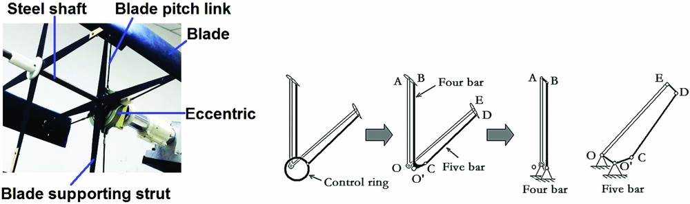
Figure 2. The control mechanism of the cycloidal propeller.
3.2 The numerical simulation model
There are three main types of turbulent modelling methods i.e. Direct Numerical Simulation (DNS), Large Eddy Simulation (LES) and Reynolds-Averaged Navier-Stokes (RANS). DNS is the most detailed approach, but it demands huge computation resources; therefore, it is too prohibitive to be used for the cases in this paper. LES is more suitable for 3D simulations and also too computationally expensive to be used for the problems in this paper. Therefore, RANS would be the best choice that incorporates both acceptable computation cost and accuracy(Reference Wang, Ingham and Ma16,Reference McNaughton, Billard and Revell18) .
Since both 2D and 3D simulations can provide acceptable accuracy(14), and the purpose of this paper is to study the effects of the dynamic stall and parallel BVI related to the pitching aerofoil in curved flow, 2D simulation, based on Fluent software, was performed in this paper.
Two coordinate systems were defined in this paper. The first one was an inertial frame whose origin is located at the axis of the cycloidal propeller. Its X and Y axes point to the vertical and horizontal directions, respectively (Fig. 3(a)). The vertical and side forces were defined in this frame. The positive vertical force points upwards along the Y axis and the positive side force points rightwards along the X axis. The resultant force of the vertical and side forces is defined as the thrust. The other one was the moving frame, which is attached to the cycloidal propeller (Fig. 3 (b)). Its origin is also located at the pitching axis of a blade. The radial and tangential force coefficients of each blade were defined in this frame. The positive radial force points outwards. The positive tangential force points to the direction of the blade tangential velocity and positive torque is in the counter-clockwise direction. Since the moving frame rotates with the shaft of the cycloidal propeller, only the pitch oscillation of each blade can be observed if the moving frame is selected as the frame of reference. This helps us to observe the effect of the dynamic stall and BVI more clearly than in the inertial frame.
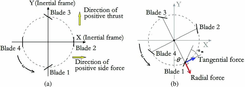
Figure 3. The definition of the coordinate system and blades.
In Fig. 3, the blades are numbered in a counter-clockwise direction. θ = 0 when blade 1 is located at the lowest point of its trajectory.
The sliding mesh technique was used to model the motion of the blade(Reference Kim, Yun and Kim3), as shown in Fig. 4. The dimension of the computation domain stretched at least 20 times the rotor diameter so that the influence of the far-field is minimised, as shown in Fig. 4(a). Unstructured mesh was deployed in the computation domain. The computation domain was subdivided into three levels of sub-domains, as shown in Fig. 4(a), (b) and (c). The sub-domain around the cycloidal propeller will rotate around the shaft of the rotor. The sub-domain around each blade will move with the moving sub-domain around the rotor, and at the same time, they will pitch around the blade pitching axis along with the blade. All these sub-domains connect with each other with mesh interfaces. The far-field condition was set to be zero pressure gradients and zero velocity. The prism elements were attached to the blade surface to capture the boundary-layer effects more efficiently, as shown in Fig. 4(d). In order to simulate the boundary-layer effects more accurately, no wall functions are used. Hence, the height of the 1st row prism elements near the blade surface was set, such that y+ is equal to or less than 1.0 and 10 rows of prism elements are deployed(19). The width of the prism elements was set, such that the aspect ratio is equal to or less than 5.0. The mesh elements were condensed around the blade and the rotor region where blade wake and vortices were expected. The total number of grid elements was of the order of 105. The Reynolds number ranges from 20 000 to 80 000; hence, the SST K-ω model with low Reynolds correction was used. This model can predict the aerofoil dynamic stall with better accuracy than that with the k-ε model and standard k-ω model(Reference Wang, Ingham and Ma16,Reference McNaughton, Billard and Revell18) . Various time step lengths were tested, and finally, it was found that the time step equal to 0.0008333Tc was fine enough to produce a time-independent solution. This corresponded to 1,200 steps per cycle, or the Courant number ⩽ 4.58 for the smallest grid in the computation domain.

Figure 4. The grid system and aerofoil used for numerical simulation.
4.0 RESULTS AND DISCUSSION
4.1 Validation of the numerical simulation model
In order to validate the numerical model employed in this paper, the simulations were performed based on the experimental cycloidal propellers, stated in Table 1. The streamline in the inertial frame revealed the same flow pattern as described in Reference Iosilevskii and LevyRef. 1, in which a distorted doublet was observed. The curved slip stream of the cycloidal propeller also can be observed from the velocity magnitude contour, as shown in Figs 5(a) and (b). When the rotation speed is 900 RPM, the tangential velocity of the blade is 17m/s. At the lowest position of the blade trajectory, the magnitude of Vy is about 8ms−1 to 16ms−1, which is comparable to blade tangential velocity, as shown in Fig. 5(b). Hence, there is strong downwash in the cycloidal rotor cage and the effective angle-of-attack (AOA) of blade 1, at this point, will be much smaller than its pitch angle.
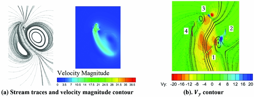
Figure 5. The velocity field of the cycloidal propeller obtained by CFD simulation (C = 70mm, 900RPM, Velocity is measured in inertial frame, θ = 3°).
The rotor aerodynamic forces obtained by CFD were validated with experimental data. The initial force measurement was performed where the centre of the eccentric lies just below the rotor shaft. It means that the blade pitch angle reaches its extreme value when it is at the highest and lowest position of its track (denoted as experiment setup 1 in Fig. 7). It was found that in this case, the CFD simulation can predict vertical force and torque well. But the side forces only qualitatively agree with the experimental results.
For the side force, the first reason for relatively larger error is that the experiment setup was not appropriate. The direction of side force actually varied from one side to another with large fluctuation and small mean value (Fig. 6(b)). Hence, for the experiment setup 1, the side force was actually fluctuating around 0. But, the force balance produces poor measurement results around zero point; therefore, the accuracy of the side force measurement was reduced.
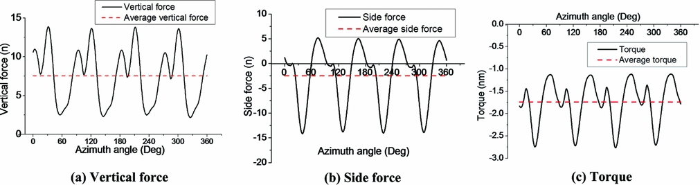
Figure 6. The forces generated by a cycloidal propeller in the inertial frame (By CFD simulation, C = 70mm, 900RPM).
Another reason for a relatively larger discrepancy between the predicted and measured side force is the fact that we are using results from a 2D solver to validate with the experiment results with a finite blade span. The effects of the finite blade span and the perpendicular BVI, due to the blade tip vortex, are ignored.
To improve the side force measurement, the position of the eccentric was turned around the rotor shaft by 90 degrees. Therefore, the blade pitch angle reaches its extreme value when it is at the leftmost and rightmost position of its track (denoted as experiment setup 2 in Fig. 7). In this case, the vertical force in experiment setup 1 was in the horizontal direction and the side force in experiment setup 1 was in the vertical direction. The weight of the cycloidal rotor system (8kg) was added to the side force so that the side force will no longer fluctuate around 0 anymore. Another benefit was that the ground effect, which was not considered in CFD simulation, can be eliminated.

Figure 7. The comparison between the experimental and CFD simulation results.
The results from CFD were compared with that from experiment setup 1 and experiment setup 2, as shown in Fig. 7. In comparison with other force components, there were still relatively larger discrepancies between predicted and measured side force. It means that in order to improve the prediction of the side force, the effect of the finite blade span and the perpendicular BVI due to blade tip vortex has to be involved into the numerical simulation. This can be addressed by a 3D numerical simulation in future work.
4.2 The force generated by a blade in one cycle
Based on numerical simulation, the vertical force generated by blade 1 can be obtained (Fig. 8). It can be noted that negative vertical force is generated during certain time intervals for each blade, which deteriorates the performance of the cycloidal propeller (Fig. 8(a)). However, the resultant vertical force generated by the cycloidal propeller is always positive and there are four pairs of vertical force peaks due to the phase shift of the blade vertical force, as shown in Fig. 6(a). The side force and torque generated by blade 1 is shown in Fig. 8(b). As shown in Figs 6(c) and 8(c), there are torque peaks due to a large fluctuation of the tangential force. This poses difficulties for stability and control of the cyclogyroes.
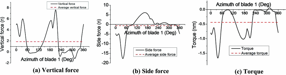
Figure 8. The forces generated by blade 1 in the inertial frame. (By CFD simulation, C = 70mm, 900RPM.)
4.3 The details of flow field around blade 1 and force generation history of blade 1 in one cycle
Based on numerical simulation, the radial force and tangential force coefficients defined in the moving frame were obtained, as shown in Fig. 9. The vertical dashed lines mark the azimuth angle corresponding to sub-figures in Fig. 10 and the letters in the parentheses under the vertical dashed lines correspond to the sub-figure IDs of Fig. 10. The vorticity contour and stream line in the moving frame are shown in Fig. 10. The vorticity in red means positive Z-vorticity and blue means negative Z-vorticity.
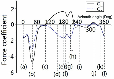
Figure 9. The radial and tangential force coefficient of blade 1 in one cycle. (By CFD simulation, C = 70mm, 900RPM.)

Figure 10. Vorticity contour and stream traces in the moving frame for test case 1 (By CFD simulation, C = 70mm, 900RPM.)
In Fig. 9, it can be seen that the radial force and tangential force coefficients are unusually high. This is because these coefficients were calculated using blade tangential speed but not the net aerodynamic velocity experienced by the blades. The relative aerodynamic velocity includes the downwash velocity in the rotor cage, and previous studies have shown that the downwash in the rotor cage is comparable to the blade tangential speed(12).
From Figs 9 and 10, it can be seen that when θ = 3°, blade 1 is located at the lowest position of its trajectory, if observed in the inertial frame (Figs 9 and 10(a)). At this position, although α p is large, the actual AOA of the blade is small, and only a very small Leading-Edge Separation Bubble (LESB) above the blade surface can be observed. This is because the downwash velocity of the flow in the cycloidal rotor cage is of the same magnitude of the tangential velocity of the blade (Fig. 5(b)). When θ ≈ 42°, the Trailing-Edge Vortex (TEV), due to dynamic stall of blade 2, approaches blade 1, and parallel BVI will occur. A strong Leading-Edge Vortex (LEV) is induced, due to the combined effect of the upwash induced by the TEV and the clockwise pitching motion of blade 1. This will result in negative radial force. At the same time, there is relatively larger inflow due to downwash in the rotor cage. The downwash also straightens the stream line so that the blade's virtual camber, due to flow curvature, is relatively smaller. However, the virtual camber at this place still helps to generate the negative radial force, which is consistent with the effects of dynamic stall and BVI. So, the combined effects of dynamic stall, parallel BVI, relatively larger inflow and virtual camber effect results in the largest radial force and tangential force peaks, as shown in Figs 9 and 10(b). Since this occurs at the lower right portion of the blade trace, this force peak results in the largest side force peak. Then, the vortices move downstream, the flow near blade 1 separates and the forces on blade 1 drop sharply. When θ ≈ 99° (Figs 9 and 10(c)), blade 1 pitches clockwise and the α p of blade 1 approaches 0. No significant aerodynamic forces are produced by blade 1. However, around this region, tangential force causes negative vertical force. Then, blade 1 goes on pitching in a clockwise direction and the α p of blade 1 increases again but changes its sign (Figs 9 and 10(d)). The LEV can be found at the bottom of blade 1. When θ = 180°, the clockwise pitching motion of blade 1 stops and the counter-clockwise pitching motion begins. The LEV causes another radial force and tangential force peak, as shown in Figs 9 and 10(e). The LEV, then, moves away from blade 1 and results in the reduction of both radial force and tangential force when θ ≈ 189° (Figs 9 and 10(f)). After this, the vortices shed from blade 2 induce parallel BVI upon blade 1. New LEV and TEV appear near blade 1, due to the upwash induced by vortices shed from blade 2. The forces on blade 1 recover at θ = 210° (Figs 9, 10(g) and 10(h)), due to the parallel BVI. Hence, parallel BVI actually can delay the stall of the blade and change the actual reduced frequency. Then, the vortices from blade 1 move away and blade 1 fully stalls (Figs 9 and 10(i)). When blade 1 continues pitching in a counter-clockwise direction, the pitch angle of blade 1 increases again. When θ = 315°, blade 1 is pitching up and a positive vertical force can be expected, but a LEV appears at the lower surface of blade 1 (Figs 9 and 10(j)) and a negative vertical force is produced. If viewed in the inertial frame, this is actually because the downwash flow in the rotor cage is blowing the blade from above, and the pitch angle of the blade is not big enough. If viewed in the moving frame, downwash causes a very large flow curvature in this area and changes the local effective AOA of the blade at the leading edge. This causes inverse AOA and positive radial force in the moving frame, or negative vertical force in the inertial frame. Therefore, the flow curvature, or the virtual camber effect, may deteriorate the performance of the cycloidal rotor in this region. After this, the LEV moves downwards and the blade is fully stalled again. When the blade continues pitching in a counter-clockwise direction, the sign of α p varies and the magnitudes of the radial force and tangential force begin to increase (Figs 9 and 10(k)). When θ = 360°, the blade starts to pitch clockwise and the next cycle begins (Figs 9 and 10(l)).
From the above discussion, it can be seen that for the cycloidal propeller with flat plate, the dynamic stall vortices on the blade cause large radial force and tangential force on the blade. The vortices shed from the upstream blade causes parallel BVI with the downstream blade. The combined effects of blade dynamic stall, parallel BVI, inflow variation and flow curvature will lead to either a drop or rise of the forces on the blade.
The force generation history is summarised in Fig. 11. It can be seen that there are two regions where intense BVI can be observed. Take blade 1 as an example – the 1st region is where the θ lies approximately between 0° and 45°. In this region, the influence of the vortices shed from blade 2 and the effect of the clockwise pitch motion of blade 1 lead to a strong LEV on blade 1. Combined with the effects of large inflow velocity caused by downwash in the rotor cage and the virtual camber effect, very large aerodynamic forces are produced (Figs 9 and 10). The 2nd region is θ approximately between 150° and 250°. In this region, multiple vortices shed from blade 2 will interact with blade 1. The interaction and the pitching motion of blade 1 result in the fluctuation of the force coefficients. A low speed region caused by downwash in the rotor cage can be observed near this region (Fig. 11(b)) and the virtual camber effect causes reverse camber in terms of vertical force generation. Hence, smaller aerodynamic forces are produced in this region. Between the 1st region and the 2nd region, blade 1 stalled first, and after that, it behaved more like an aerofoil undergoing pitch up motion with dynamic stall. Between the 2nd region and the end of the cycle, the blade stalled and then negative vertical force was generated, due to downwash or very high flow curvature in the rotor cage. Fortunately, the blade is travelling in the low speed region, as shown in Fig. 11(b), and aerodynamic forces will be relatively small if the leading edge of the blade does not stretch too far forward. After this, the blade will gain vertical force again and the next cycle will begin.
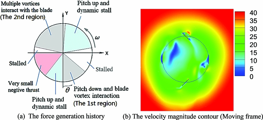
Figure 11. Demonstration of force generation history of blade 1 in one cycle.
The scaled radial force, tangential force and their resultant force are shown in Fig. 12. It is clear that most of the aerodynamic force is generated when blade 1 is at the upper and bottom position in the inertial frame. When the blade is at the left and right side, the force vectors can be barely seen. In most periods, if the magnitude of the tangential force and radial force are of the same order, it means that the cycloidal rotor generates a large thrust with a very large torque.

Figure 12. The scaled force vectors of blade 1 at different azimuth angle. (By CFD simulation, C = 70mm, 900RPM.)
The power loading can be expressed in the following from Reference LeishmanRef. 20:
 $$\begin{equation}
{\rm{PL}} = \frac{T}{P} = \frac{T}{{Q \times \omega }}
\end{equation}$$
$$\begin{equation}
{\rm{PL}} = \frac{T}{P} = \frac{T}{{Q \times \omega }}
\end{equation}$$
T/Q of the cycloidal rotor is low, but in comparison with a screw propeller working at the same disc loading, the cycloidal propeller works at a very low rotation speed. Therefore, the cycloidal propeller still has at least comparable efficiency to that of a screw propeller. This might be caused by the following factors:
-
1. The blade dynamic stall, BVI, inflow variation and virtual camber effect lead to very large aerodynamic force and thrust. In the test case stated above, the maximum Cn is almost 5.0 and the average Cn is 1.0035;
-
2. The parallel BVI between the dynamic stall vortices and downstream blade will induce downwash and upwash on the downstream blade. There are new LEVs on the downstream blade and they induce new force peaks. This actually delays the stall of the blade;
-
3. For the conventional screw propeller, most of the thrust is generated by the blade elements located near the blade tip. The blade elements near the rotor hub suffer from low speed and relatively lower efficiency. But for the cyclorotor, the entire blade is working at the same speed at the periphery of the rotor; therefore, the cycloidal propeller can generate a high thrust at a very low rotation speed. And just as described in Ref. 12, each span-wise blade element of a cyclorotor operates at similar aerodynamic conditions, so the blades can be more easily optimised to achieve best aerodynamic efficiency.
5.0 CONCLUSIONS
The numerical simulation and analysis based on 2D RANS model were performed on a cycloidal rotor with a 2mm flat plate aerofoil and a chord length of 70mm. The following conclusions can be drawn based on the test case stated in this paper:
-
1. The dynamic stall can be observed due to the pitching motion of the blade. There are intense parallel BVI induced by dynamic stall vortices at the upper left and lower right part of the blade trace. Parallel BVI can change the effective AOA and reduced frequency of the blade. These effects result in high-force coefficient peaks. Therefore, most of the aerodynamic force is generated when a blade travels through the upper and lower part of its trace. The parallel BVI also helps delay the stall of the blade, which is beneficial to the thrust generation.
-
2. There is downwash in the rotor cage whose velocity is comparable to the blade tangential velocity. The downwash will change the magnitude and direction of the inflow velocity experienced by the blade, and vary the flow curvature or virtual camber if observed in the moving reference frame. The flow curvature can be either beneficial or harmful to the thrust generation, depending on the location of the blade and its leading edge. Downwash and flow curvature may either help to generate very large aerodynamic force peak, which is beneficial to thrust generation, or cause negative vertical force, which is harmful to thrust generation.
-
3. The combined effects of dynamic stall, parallel BVI, inflow variation and flow curvature (or virtual camber effect) induce very large aerodynamic force over the blade. Combined with the fact that the entire blade works in a similar condition, the cycloidal propeller can produce high thrust at a very low rotation speed. This ensures that the hovering efficiency of the cycloidal propeller is at least comparable to that of the screw propeller, although the torque of the cycloidal rotor blade is very large. On the other hand, very large fluctuation of the aerodynamic force causes vibration and poses difficulties for stability and control of the cyclogyro.