Nomenclature
Abbreviations
- BE
-
Boltzmann Equation
- DSMC
-
Direct Simulation Monte Carlo
- MD
-
Molecular Dynamics
- NSF
-
Navier-Stokes Fourier
- PPC
-
Particles Per Cell
Symbols
-
 $c^{\prime} $
-
Thermal velocity of the molecules [m/s]
-
$C_p $
-
Pressure coefficient
-
$C_f $
-
Skin friction coefficient
-
$C_h $
-
Heat transfer coefficient
-
$ d$
-
Molecular diameter [m]
-
$ f$
-
Distribution function
-
$ h$
-
Characteristic length-(Step height) [m]
- H
-
Channel height at outlet [m]
-
$k_b $
-
Boltzmann constant
-
$ Kn$
-
Knudsen Number
-
$ m$
-
Molecular mass [kg]
-
$M $
-
Mach Number
-
$ n$
-
Number density [
$\textrm{m}^{-3} $
] -
$ N$
-
Number of molecules
-
$ P$
-
Pressure [N/m2]
-
$ q$
-
Heat flux [W/m2]
-
$ R$
-
Gas constant [J/mol. K]
-
$ Re$
-
Reynolds Number
-
$t $
-
Time [s]
-
$ T$
-
Temperature [K]
- X
-
Distance in x-direction [m]
- Y
-
Distance in y-direction [m]


Greek Symbols
-
$\chi $
-
Mole fraction
-
$\omega $
-
Viscosity-temperature index
-
$\rho $
-
Density of the gas [kg/m3]
-
$ \mu $
-
Viscosity of the gas [N.s/m2]
-
$\tau $
-
Shear stress [N/m2]
-
$\lambda $
-
Mean free path [m]
-
$\varsigma $
-
Degree of freedom
-
$ \Delta $
-
Timestep
-
$\Theta $
-
Vibrational temperature
-
$ \delta $
-
Boundary layer thickness


Subscripts
-
$\infty $
-
Free stream
-
$s $
-
Slip
-
$j $
-
Jump
-
$w $
-
Wall
-
$ R$
-
Rotational
-
$T $
-
Translational
-
$V $
-
Vibrational
-
$ov $
-
Overall


1.0 Introduction
The aerospace vehicles that enter the earth from outer space require extensive research in rarefied gas flow dynamics. Generally, such vehicles operate at hypersonic speeds (Mach number of above 5), at higher altitudes, and encounter a rarefied flow environment. Furthermore, they usually experience different rarefaction regimes, ambient temperatures, and intricate flow patterns, including shocks [Reference Guo and Luo1]. Also, the chemical reactions at higher altitudes influence the flow field properties [Reference Gallis, Bond and Torczynski2]. While it is desirable to have a smooth aerodynamic surface shape, several irregularities exist on such vehicles in the form of steps, contours, gaps during their development stage or flight. These abnormalities arise due to sensor installations, manufacturing tolerances and the placement of thermal protection system tiles [Reference Palharini, Scanlon and Reese3]. Such abnormalities in advanced aerodynamic configurations lead to flow separation [Reference Morgan, Periaux and Thomasset4, Reference Chen, Asai, Nonomura, Xi and Liu5]. The backward-facing step (BFS) is one of such simplified irregularities, which is mainly explored. The investigation into the BFS flow also has many practical applications in various fields [Reference Leite and Santos6]. Therefore, in this paper, the rarefaction effects on the flow behaviour past a BFS are addressed. The Knudsen number (
 $Kn$
) is employed to estimate the flow rarefaction and is given by [Reference Ahmadian, Roohi, Teymourtash and Stefanov7].
$Kn$
) is employed to estimate the flow rarefaction and is given by [Reference Ahmadian, Roohi, Teymourtash and Stefanov7].
 \begin{align}Kn = \frac{{\rm{\lambda }}}{{\rm{h}}}\end{align}
where,
 ${\rm{\lambda }}$
depicts the mean free path, and
${\rm{\lambda }}$
depicts the mean free path, and
 $h$
is the characteristic dimension of the geometry under consideration. In the present work,
$h$
is the characteristic dimension of the geometry under consideration. In the present work,
 $h$
is the step height.
$h$
is the step height.
The Knudsen number classifies the flow regimes as [Reference Mohammadzadeh, Roohi, Niazmand, Stefanov and Myong8]:
 $Kn \le 0.001$
(Continuum regime),
$Kn \le 0.001$
(Continuum regime),
 $0.001 \le Kn \le 0.1$
(Slip regime),
$0.001 \le Kn \le 0.1$
(Slip regime),
 $0.1 \le Kn \le 10$
(Transitional regime) and
$0.1 \le Kn \le 10$
(Transitional regime) and
 $Kn \ge 10$
(free-molecular regime). The breakdown of continuum theory occurs as the flow approaches the slip regime owing to prevalent rarefaction results, thereby requiring the use of computational alternatives, such as the solution of Boltzmann equations (BE), direct simulation Monte Carlo (DSMC), and Molecular dynamics (MD).
$Kn \ge 10$
(free-molecular regime). The breakdown of continuum theory occurs as the flow approaches the slip regime owing to prevalent rarefaction results, thereby requiring the use of computational alternatives, such as the solution of Boltzmann equations (BE), direct simulation Monte Carlo (DSMC), and Molecular dynamics (MD).
The Knudsen number (
 $Kn$
), Reynolds number
$Kn$
), Reynolds number
 $\left( {{\rm{Re}}} \right),$
and Mach number
$\left( {{\rm{Re}}} \right),$
and Mach number
 $\left( {\rm{M}} \right)$
are related to each other as follows:
$\left( {\rm{M}} \right)$
are related to each other as follows:
 \begin{align}Kn = \sqrt {{{\pi \gamma } \over 2}} {{\rm{M}} \over {{\rm{Re}}}}\,{\rm{where}}\,{\rm{M}} = {{{U_\infty }} \over {\sqrt {\gamma RT} }}\,{\rm{and}}\,{\rm{Re}} = {{\rho {U_\infty }h} \over \mu }\end{align}
where ρ represents the density,
 ${U_\infty }$
the free-stream velocity,
${U_\infty }$
the free-stream velocity,
 $h$
is the step height, and
$h$
is the step height, and
 $\mu $
is the dynamic viscosity of the fluid, and R denotes the gas constant.
$\mu $
is the dynamic viscosity of the fluid, and R denotes the gas constant.
The BFS is an interesting configuration due to the prevalence of flow separation and reattachment. Numerous investigations have been performed to comprehend the phenomenon of flow separation and reattachment over BFS. The studies regarding the effect of aspect ratio, Prandtl number, Reynold’s number, and step height have been documented using numerical and analytical methods for 3D and 2D flow to further our understanding of the BFS. In general, near-space corresponds to a region where its altitude ranges from 20 kilometers to 100 kilometers [Reference Nabapure and Kalluri16] and attracts greater focus in modern times because of the defense applications. Many researchers have documented numerous investigations involving both experimental and computational approaches involving flow over basic geometries. The studies carried out also include the BFS flow in the subsonic [Reference Darbandi and Roohi19, Reference Mahdavi and Roohi20], supersonic [Reference Mahdavi, Le, Roohi and White21, Reference Gavasane, Agrawal and Bhandarkar22] and hypersonic [Reference Guo, Liu and Zhang23, Reference Paolicchi and Santos24] domains, though most of them are in the continuum regime. Therefore, a few significant studies are discussed in this introduction.
Choi et al. [Reference Choi, Lee and Lee9] implemented a compressible Navier-Stokes Fourier (NSF) equation with Langmuir slip boundary condition for the BFS flow and accurately predicted the flow physics. Hsieh [Reference Hsieh, Hong and Pan10] investigated the 3D microscale BFS flow using the DSMC method. The study was carried out by simplifying the 3D configuration to 2D, and they examined the flow separation, recirculation and reattachment. Beskok [Reference Beskok11] devised a velocity-slip boundary condition and applied the same for the BFS flows. Similarly, Celik and Edis [Reference Celik and Edis12] formed the Finite element form of the Navier-Stokes equation and implemented it for the BFS flows. Rached and Daher [Reference Rached and Daher13] used the conventional control-volume approach with slip/jump boundary conditions to explore the BFS flow. They compared their results with analytical findings and found a good agreement with each other. An analogous procedure for BFS was implemented by Baysal et al. [Reference Baysal, Erbas and Koklu14]. Xue and Chen [Reference Xue and Chen15] used the DSMC method for flow past BFS on a microscale and investigated the rarefaction effects. Their outcomes indicated that the flow phenomena such as flow separation, reattachment and recirculation disappeared when
 $Kn$
exceeded 0.1. Xue et al. [Reference Xue and Chen15] explained the reasons for the above phenomena in another study.
$Kn$
exceeded 0.1. Xue et al. [Reference Xue and Chen15] explained the reasons for the above phenomena in another study.
Nabapure and Kalluri [Reference Nabapure and Kalluri16] investigated the compressibility and effect of wall temperature on the hypersonic BFS flow using the DSMC method. Kursun and Kapat [Reference Kursun and Kapat17] used the DSMC-IP (Information preservation) method to investigate BFS flows. They carried out the studies for
 ${\rm{Re}}$
of 0.03 to 0.64,
${\rm{Re}}$
of 0.03 to 0.64,
 ${\rm{M}}$
of 0.013 to 0.083. For the above conditions, they did not report any recirculation region. Bao and Lin [Reference Bao and Lin18] studied the microscale-BFS flows using the continuum-based Burnett equations. They correlated their numerical findings with the available experimental and numerical results from the literature, which showed good agreement. Darbandi and Roohi [Reference Darbandi and Roohi19] employed the DSMC technique to investigate the micro/nano-BFS flows in the subsonic domain and investigated the effect of rarefaction. Their results indicated a decrease in the separation region length as the flow entered the transitional regime. Mahadavi and Roohi [Reference Mahdavi and Roohi20] analysed the effects of rarefaction, pressure ratio and wall temperature for nano BFS flow using DSMC and studied the flow behaviour. Mahadavi et al. [Reference Mahdavi, Le, Roohi and White21] analysed the micro/nano BFS by incorporating hybrid slip/jump boundary conditions in the NSF equations and evaluated the influence of various pressure ratios, inlet temperatures and wall temperatures. The results of their modified boundary condition predicted better compared to DSMC. Gavasane et al. [Reference Gavasane, Agrawal and Bhandarkar22] also used the DSMC method and analysed the rarefaction and pressure ratio effects on the micro-BFS with Argon as the fluid. Guo et al. [Reference Guo, Liu and Zhang23] employed the DSMC method to investigate the BFS flow in the slip and transitional flow regime and explored the various flow characteristics. Leite et al. [Reference Leite and Santos6] used the DSMC technique to analyse the hypersonic BFS flow with non-reacting air as the fluid and inspected the aerodynamic properties for different step heights.
${\rm{M}}$
of 0.013 to 0.083. For the above conditions, they did not report any recirculation region. Bao and Lin [Reference Bao and Lin18] studied the microscale-BFS flows using the continuum-based Burnett equations. They correlated their numerical findings with the available experimental and numerical results from the literature, which showed good agreement. Darbandi and Roohi [Reference Darbandi and Roohi19] employed the DSMC technique to investigate the micro/nano-BFS flows in the subsonic domain and investigated the effect of rarefaction. Their results indicated a decrease in the separation region length as the flow entered the transitional regime. Mahadavi and Roohi [Reference Mahdavi and Roohi20] analysed the effects of rarefaction, pressure ratio and wall temperature for nano BFS flow using DSMC and studied the flow behaviour. Mahadavi et al. [Reference Mahdavi, Le, Roohi and White21] analysed the micro/nano BFS by incorporating hybrid slip/jump boundary conditions in the NSF equations and evaluated the influence of various pressure ratios, inlet temperatures and wall temperatures. The results of their modified boundary condition predicted better compared to DSMC. Gavasane et al. [Reference Gavasane, Agrawal and Bhandarkar22] also used the DSMC method and analysed the rarefaction and pressure ratio effects on the micro-BFS with Argon as the fluid. Guo et al. [Reference Guo, Liu and Zhang23] employed the DSMC method to investigate the BFS flow in the slip and transitional flow regime and explored the various flow characteristics. Leite et al. [Reference Leite and Santos6] used the DSMC technique to analyse the hypersonic BFS flow with non-reacting air as the fluid and inspected the aerodynamic properties for different step heights.
Also, various works have investigated the flow over cavities. Palharini et al. [Reference Palharini, Scanlon and Reese3] used the DSMC method to study the impact of three-dimensionality on the aerodynamic characteristics of the cavity flow. Santos et al. [Reference Paolicchi and Santos24] used the DSMC technique to investigate the effect of changing cavity height on the aerodynamic characteristics of a hypersonic cavity flow. Guo et al. [Reference Guo and Luo1] used the DSMC method to study rarefied flow across different cavity shapes and studied the flow field characteristics. In another study, Guo et al. [Reference Guo and Luo25] examined the flow-field properties of a 2D hypersonic cavity flow for different Knudsen numbers within the transitional regime. In similar research, Palharini et al. [Reference Palharini and Santos26] used the DSMC technique to investigate the impact of changing cavity length for various (L/D) (length to depth) ratios in the cavity in the transitional regime. Jin et al. [Reference Jin, Wang, Cheng, Wang and Huang27] used the DSMC method to investigate the effect of the Maxwellian accommodation coefficient on rarefied hypersonic flows across 3D cavity flows in the transitional regime.
Based on the above review, significant research exists on the rarefied flow over a BFS in different flow regimes. Nonetheless, the aerothermodynamic conditions encountered by hypersonic re-entry vehicles are challenging to analyse owing to the various complexities involved, which are not adequately recorded in the open literature. Most of the past research primarily concentrated on investigating the rarefaction effects at lower Knudsen numbers. Moreover, only a handful of studies have analysed the range of rarefaction regimes that the hypersonic re-entry vehicles encounter, but they are limited to the transitional flow regime. However, the re-entry vehicles typically experience higher levels of rarefaction at higher altitudes, and the rarefaction levels reduce as they descend back to the earth. However, to the best of the authors’ knowledge, none of the previous investigations provide a comprehensive analysis of the effects of rarefaction on the flow and surface properties that a re-entry vehicle typically encounters during its flight, particularly in the free molecular regime. Thus, this paper aims to bridge the gap and explores the flow-field and aerodynamic properties for a range of Knudsen numbers covering different flow regimes from the slip to free-molecular.
Therefore, in the present analysis, we use the DSMC approach by adopting an open-source solver named dsmcFoam to analyse the rarefaction effects for flow over a BFS. The research objectives are to (i) to examine the rarefaction effects by considering a range of Knudsen numbers covering the slip to free-molecular regimes, (ii) to study the variation of the flow and surface properties at various locations along the transverse direction, (iii) to examine the recirculation regions formed and estimate the recirculation lengths for the different regimes (iv) to compare the non-reacting flows against the reacting flows and outline the differences.
2.0 Numerical methodology
In this section, the computational domain, a brief description of the computational approach employed for the analysis, and the various computational parameters used in the investigation are provided.
2.1 DSMC
Bird [Reference Bird28] introduced the direct simulation Monte Carlo (DSMC) technique in the mid-1960s, which is regarded as one of the most robust approaches for solving the Boltzmann equation. The DSMC solution is a useful computational method for simulating rarefied gas flows, whether reactive or not. This approach guides molecules into stages of decoupling, motion, and collision, using the kinetic theory to obtain non-continuum gas characteristics accurately. The DSMC is mainly used in simulating high-speed rarefied gas flows having higher levels of rarefaction.
As known, the air density declines steadily as the elevation rises, and the rarefaction effects influence the flow properties. Also, there is a breakdown of NSF equations [Reference Mohammadzadeh, Roohi, Niazmand, Stefanov and Myong8], paving the way for the usage of the Boltzmann equation given as [Reference Zhang, Liu and Jin29]:
 \begin{align}{{\partial f} \over {\partial t}} + v.{\nabla _x}f = {1 \over {Kn}}Q\left( {f,f} \right)\!,\,x \in {{\mathbb R}^{dx}},\,v \in {{\mathbb R}^{dv}}\end{align}
where
 $f\!\left( {t,x,v} \right)$
denotes the density distribution function of a dilute gas at a position
$f\!\left( {t,x,v} \right)$
denotes the density distribution function of a dilute gas at a position
 $x$
, velocity
$x$
, velocity
 $v$
and at time
$v$
and at time
 $t$
.
$t$
.
 $Kn$
represents the Knudsen number of the flow and the collision operator
$Kn$
represents the Knudsen number of the flow and the collision operator
 $Q\left( {f,f} \right)$
denotes the binary collisions taking place.
$Q\left( {f,f} \right)$
denotes the binary collisions taking place.
The basic rules of the DSMC approach comprise four main aspects: moving, indexing, collision and sampling. The DSMC scheme employs a mathematical framework that models the actual gas dynamics by the movement of various simulated particles represented as a conglomeration of several actual particles and determines their interactions. A parallel DSMC package is used in the current analysis to save computing power by utilising 32 cores. The computational domain comprising a structured 2D grid is split into cells for choosing the collision pairs. There are many schemes to select a collision pair; a review is given in Refs [Reference Roohi and Stefanov30, Reference Roohi, Stefanov, Shoja-Sani and Ejraei31]. Here the No Time Counter scheme(NTC) [Reference Abe32] is selected. Also, DSMC has a variety of collision models, which are explained in Ref. (Reference Prasanth and Kakkassery33). The current study handles the intermolecular collisions using the Variable Hard Sphere (VHS) collision model.
The DSMC approach primarily depends on the proper selection of the cell size, particles per cell, and time step for generating accurate results. The cell size is usually chosen to be smaller than a third of the mean free path [Reference Alexander, Garcia and Alder34], and similarly, the time step is smaller than a third of the collision’s mean time [Reference Hadjiconstantinou35]. The above criteria are adapted in the present study. The particles per cell were 25 providing sufficient accuracy.
In this study, DSMC computations employed the open-source dsmcFoam code [Reference Scanlon, Roohi, White, Darbandi and Reese36, Reference White37]. The code is highly efficient and scalable by adapting efficient parallelisation techniques such as OpenMPI. Moreover, the code has been validated on various problems in rarefied gas flows.
2.2 Geometry and computational domain
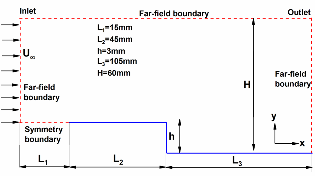
The rarefied flow over a 2D BFS, as shown in Fig. 1, is the geometry considered for analysis. The study is conducted for a range of Knudsen numbers where the flow moves from left to right.
 $X$
and
$X$
and
 $Y$
denote the cartesian coordinates along the streamwise and transverse directions. The upstream length was kept at 60mm, including an initial 15mm length of the symmetry region. The downstream length considered was 105mm, and the step was located at 60mm from the inlet and is far enough from both the inlet and outlet. For all simulations, the step height (
$Y$
denote the cartesian coordinates along the streamwise and transverse directions. The upstream length was kept at 60mm, including an initial 15mm length of the symmetry region. The downstream length considered was 105mm, and the step was located at 60mm from the inlet and is far enough from both the inlet and outlet. For all simulations, the step height (
 $h$
) was set at 3mm. The channel height at the outlet was fixed at
$h$
) was set at 3mm. The channel height at the outlet was fixed at
 ${\rm{H}} = 60{\rm{mm}}$
after conducting a domain independence study such that the top surface does not influence the flow-field and surface properties. The range of
${\rm{H}} = 60{\rm{mm}}$
after conducting a domain independence study such that the top surface does not influence the flow-field and surface properties. The range of
 $Kn$
studied was 0.05, 0.1, 1.06, 10.33, 21.10, covering all the rarefaction regimes.
$Kn$
studied was 0.05, 0.1, 1.06, 10.33, 21.10, covering all the rarefaction regimes.

Figure 1. Schematic of the 2D BFS.
2.3 Boundary conditions and mesh
The different boundary conditions applied on the surfaces are, as shown in the computational domain in Fig. 1. The left, top, and right boundaries represent the far-field boundary condition through which the simulated particles easily enter and leave the domain. The solid boundary (blue) represents the BFS and is given a diffused reflection with full thermal accommodation condition. In a diffuse reflection model, the simulated molecules are equally reflected in all directions. The initial length of 15mm from the inlet to the edge of the flat plate represents symmetry and is used to accomplish a precise velocity in the perpendicular directions [Reference Roohi and Stefanov30]. Thus, this surface is analogous to a specular reflecting model.
The computational domain is divided into several blocks and meshed in a structured manner, as shown in Fig. 2. The cell widths in both
 $X$
and
$X$
and
 $Y$
directions were maintained below the mean free path, i.e.
$Y$
directions were maintained below the mean free path, i.e.
 ${\rm{\Delta }}{x_{cell}}$
,
${\rm{\Delta }}{x_{cell}}$
,
 ${\rm{\Delta }}{y_{cell}}$
< 0.3
${\rm{\Delta }}{y_{cell}}$
< 0.3
 ${\lambda _\infty }$
. The total number of cells for the case of
${\lambda _\infty }$
. The total number of cells for the case of
 $Kn = 1.06$
was about 11,250 cells. Also, the cell count varied for other cases depending on the corresponding mean free path.
$Kn = 1.06$
was about 11,250 cells. Also, the cell count varied for other cases depending on the corresponding mean free path.
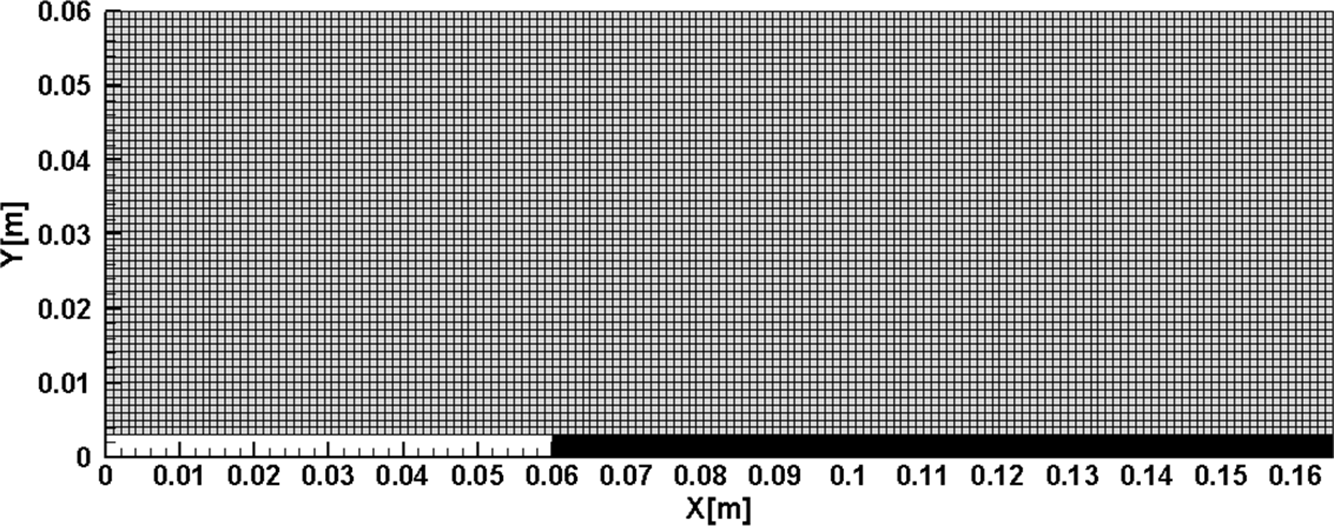
Figure 2. Meshed domain.
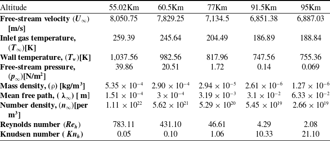
Tables 1 and 2 show the gas properties and the free-stream flow parameters employed in the present simulations. Such flow characteristics are experienced by a hypersonic vehicle during its re-entry and are taken from the U.S. Standard Atmosphere charts [38]. In the initial studies, the fluid considered was non-reacting air, and the chemical reactions were relaxed. This assumption has been used in numerous published studies [Reference Palharini, Scanlon and Reese3, Reference Palharini and Santos26, Reference Jin, Wang, Cheng, Wang and Huang27, Reference Leite and Santos39]. Also, the fluid was assumed to have a molecular weight of about 28.96 g/mol with a major composition of 76%
 ${{\rm{N}}_2}$
and 23%
${{\rm{N}}_2}$
and 23%
 ${{\rm{O}}_2}$
. The inflow free stream
${{\rm{O}}_2}$
. The inflow free stream
 $M$
was set as 25 and was constant for all cases. The literature has various studies where the Mach number of 25 was considered [Reference Palharini and Santos26, Reference Leite and Santos39]. Also, since these vehicles travel at speeds greater than Mach 25, the downstream body surface still experiences velocities around Mach 25. Alternatively, the flow can be impinging at an angle in which case the flow directly encounters the BFS. Sharp or slender objects are other instances with a weak bow shock, which could result in the situation that is considered in the present study. All the wall surfaces
$M$
was set as 25 and was constant for all cases. The literature has various studies where the Mach number of 25 was considered [Reference Palharini and Santos26, Reference Leite and Santos39]. Also, since these vehicles travel at speeds greater than Mach 25, the downstream body surface still experiences velocities around Mach 25. Alternatively, the flow can be impinging at an angle in which case the flow directly encounters the BFS. Sharp or slender objects are other instances with a weak bow shock, which could result in the situation that is considered in the present study. All the wall surfaces
 $({T_w})$
were maintained at four times the free-stream temperature
$({T_w})$
were maintained at four times the free-stream temperature
 $4{T_\infty }$
.
$4{T_\infty }$
.
Table 1. Gas properties [Reference Leite and Santos39]
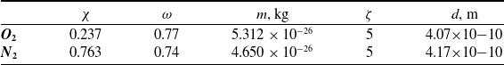
Table 2. Flow and simulation parameters [38]

In Table 1,
 ${\rm{\chi }}$
denotes the mole fraction,
${\rm{\chi }}$
denotes the mole fraction,
 $m$
denotes the molecular mass,
$m$
denotes the molecular mass,
 $d$
the molecular diameter,
$d$
the molecular diameter,
 $\omega$
represents the temperature dependent viscosity index, and
$\omega$
represents the temperature dependent viscosity index, and
 $\zeta $
represents the degrees of freedom.
$\zeta $
represents the degrees of freedom.
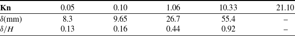
Table 2 lists the flow and simulation parameters, which show the different atmospheric altitudes examined, ranging from 55Km to 95Km. All the simulations ran for about
 $1.5{\rm{ms}}$
, which consisted of 75,000 timesteps and employed about 276,500 simulated particles. The time averaging of the DSMC particle fields was started once the total DSMC particles reached a steady state. The solution was considered steady-state when the average linear kinetic energy of the system showed no significant variation [Reference Scanlon, Roohi, White, Darbandi and Reese36]. The Knudsen number (
$1.5{\rm{ms}}$
, which consisted of 75,000 timesteps and employed about 276,500 simulated particles. The time averaging of the DSMC particle fields was started once the total DSMC particles reached a steady state. The solution was considered steady-state when the average linear kinetic energy of the system showed no significant variation [Reference Scanlon, Roohi, White, Darbandi and Reese36]. The Knudsen number (
 $K{n_h}$
) and Reynolds number
$K{n_h}$
) and Reynolds number
 $\left( {{\rm{R}}{{\rm{e}}_h}} \right)$
were estimated by choosing the step height (h) as the characteristic dimension.
$\left( {{\rm{R}}{{\rm{e}}_h}} \right)$
were estimated by choosing the step height (h) as the characteristic dimension.
In the later part of the study, the comparison of chemically reacting flows with non-reacting flows was carried out. This section briefly describes the details of the chemical modeling. Several chemical reaction models, like the Total Collision Energy (TCE) model, introduced by Bird [Reference Bird40], are available in the DSMC. Predominantly the popular TCE utilises the equilibrium kinetic theory to correlate the macroscopic and microscopic properties of the gas by translating the Arrhenius rate coefficients into collision probabilities, which are a function of macroscopic gas temperature and microscopic collision energy, respectively. In recent years, an alternative reaction model, the Quantum-Kinetic (Q-K) chemistry model, was proposed by Bird [Reference Bird41]. This model is used in the present study and has been employed in dsmcFoam+ code.
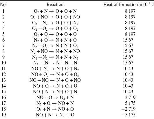
The Q-K method is a molecular level chemistry model that employs the fundamental molecular properties, antithetical to the classical TCE model, which relies on experimental data availability. In this study, the Q-K chemistry model has been used to define the chemical reactions of a five-species air model with a total of 19 chemical reactions in the dsmcFoam+. Two chemical reaction types are relevant to the present discussion: Dissociation (No. 1–15 in Table 3) and Exchange reactions (No. 16–19 in Table 3).
Table 3. List of chemical reactions employed

The overall temperature is defined as the weighted average of translational, rotational, and vibrational temperatures [Reference Bird42] and is given by,
 \begin{align}{T_{ov}} = \frac{{3{T_T} + {\xi _R}{T_R} + {\xi _V}{T_V}}}{{3 + {\xi _R} + {\xi _V}}}\end{align}
where
 $\xi $
is the degree of freedom and the subscripts
$\xi $
is the degree of freedom and the subscripts
 $T$
,
$T$
,
 $R$
and
$R$
and
 $V$
stand for translation, rotation and vibration, respectively.
$V$
stand for translation, rotation and vibration, respectively.
The following equations give the translational, rotational and vibrational temperatures,
 \begin{align}{T_T} = {1 \over {3{k_b}}}{{\mathop \sum \nolimits_{j = 1}^N {m_j}c{'^2}} \over N}\end{align}
 \begin{align}{T_R} = \frac{2}{{{k_b}{\xi _R}}}\frac{{\mathop \sum \nolimits_{j = 1}^N {{({\varepsilon _R})}_j}}}{N}\end{align}
 \begin{align}{T_V} = \frac{{{{\rm{\Theta }}_V}}}{{{\rm{ln}}\left( {1 + \frac{{{k_b}{{\rm{\Theta }}_V}}}{{\mathop \sum \nolimits_{j = 1}^N {{({\varepsilon _V})}_j}}}} \right)}}\end{align}
where
 ${k_b}$
is the Boltzmann constant,
${k_b}$
is the Boltzmann constant,
 ${\varepsilon _R}$
and
${\varepsilon _R}$
and
 ${\varepsilon _V}$
represent the average rotational and vibrational energies and
${\varepsilon _V}$
represent the average rotational and vibrational energies and
 ${{\rm{\Theta }}_V}$
denotes the characteristic vibrational temperature, which has a value of 3,371K and 2,256K for
${{\rm{\Theta }}_V}$
denotes the characteristic vibrational temperature, which has a value of 3,371K and 2,256K for
 ${N_2}$
and
${N_2}$
and
 ${O_2}$
respectively. The rotational and vibrational collision relaxation number considered in the study was 5 and 50, respectively.
${O_2}$
respectively. The rotational and vibrational collision relaxation number considered in the study was 5 and 50, respectively.
3.0 Model validation and verification
In the section, the validation studies performed to assess the accuracy of the solver are explained. Without considering the chemical reactions, the validation was performed for a comparable case of flow over a BFS. Furthermore, the solver was validated, accounting for the chemical reactions using a cylinder test case. Also, the verification studies carried out to predict the results accurately are presented.
3.1 Validation
3.1.1 Flow over BFS
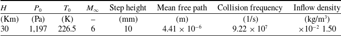
In the present study, the investigations are performed by utilising the dsmcFoam solver. The solver has been validated for different cases [Reference Nabapure, Sanwal, Rajesh and Murthy43–Reference Nabapure and Murthy51]. For the comparable case of flow over BFS, the results predicted by the current model using the DSMC method are compared with the numerical results of Guo et al. [Reference Guo, Liu and Zhang23]. Guo et al. [Reference Guo, Liu and Zhang23] investigated the flow characteristics of a hypersonic BFS of step height 10mm in the slip and transitional regime using the DSMC method. The simulation parameters adopted for the case of
 ${\rm{H}} = 30{\rm{Km}}$
are shown in Table 4. For visual validation, the velocity contours reported by Guo et al. were compared and are presented in Fig. 3, which shows a good agreement.
${\rm{H}} = 30{\rm{Km}}$
are shown in Table 4. For visual validation, the velocity contours reported by Guo et al. were compared and are presented in Fig. 3, which shows a good agreement.
Table 4. Computational details of Guo et al. [Reference Guo, Liu and Zhang23]

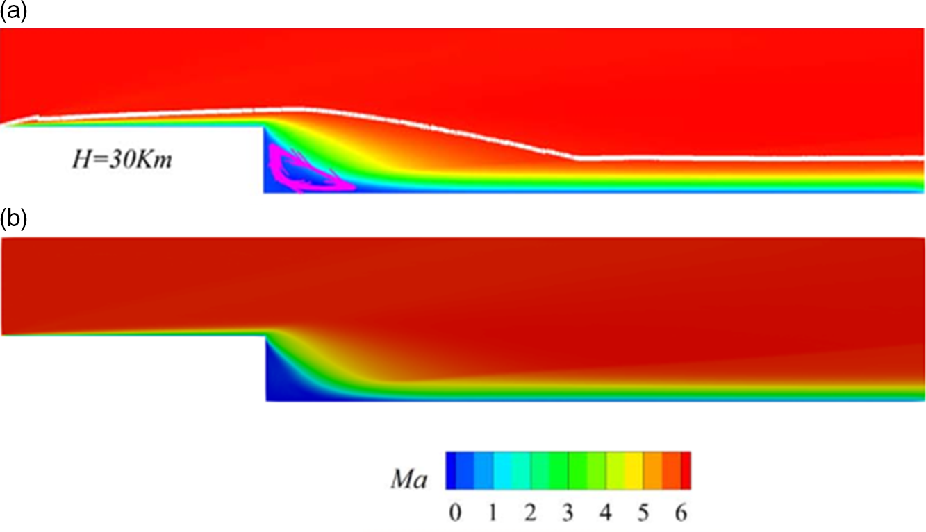
Figure 3. Comparison of velocity contour for the case of
 $H = 30{\rm{Km}}$
(a) published results [Reference Guo, Liu and Zhang23] (b) simulation results.
$H = 30{\rm{Km}}$
(a) published results [Reference Guo, Liu and Zhang23] (b) simulation results.
Additionally, the streamwise velocity and the pressure normal to the BFS surface at
 $X/h = 5$
are shown in Fig. 4. Where
$X/h = 5$
are shown in Fig. 4. Where
 $X$
represents the axial distance normalised by the free-stream step height (
$X$
represents the axial distance normalised by the free-stream step height (
 $h$
). From the streamwise velocity profile, it is observed that both the results show reasonable agreement, with a slight discrepancy near the wall. Also, the comparison of the pressure shows a fair match between our results with the published results. Thus, our findings match well with Guo et al., thus validating the current study’s numerical model.
$h$
). From the streamwise velocity profile, it is observed that both the results show reasonable agreement, with a slight discrepancy near the wall. Also, the comparison of the pressure shows a fair match between our results with the published results. Thus, our findings match well with Guo et al., thus validating the current study’s numerical model.
3.1.2 Chemically reacting flow over a circular cylinder
To validate the solver incorporating the chemical reactions, a test case of the cylinder was simulated. A two-dimensional hypersonic rarefied air flow over a circular cylinder with a diameter of 2m, investigated by Scanlon et al. [Reference Scanlon52], was used as a benchmark case, and the Quantum-Kinetics (Q–K) chemical reaction model was considered. The free-stream and flow conditions for atmospheric altitude,
 $H = 86{\rm{Km}}$
, are shown in Table 5. Figure 5(a) compares Mach number contours reported by Scanlon et al. and the present simulation. Figure 5(b) depicts the species’ number density along the stagnation line in front of the cylinder. The results obtained match well with the Q–K results of Scanlon et al., thus, supporting the validity of our results for chemically reacting rarefied flow in the present work.
$H = 86{\rm{Km}}$
, are shown in Table 5. Figure 5(a) compares Mach number contours reported by Scanlon et al. and the present simulation. Figure 5(b) depicts the species’ number density along the stagnation line in front of the cylinder. The results obtained match well with the Q–K results of Scanlon et al., thus, supporting the validity of our results for chemically reacting rarefied flow in the present work.
Table 5. Computational details of Scanlon et al. [Reference Scanlon52]
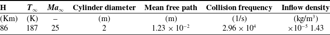
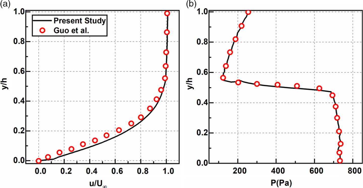
Figure 4. Comparison of (a) streamwise velocity and (b) pressure along the vertical line of
 $X/h = 5$
for the case of
$X/h = 5$
for the case of
 $H = 30{\rm{Km}}$
.
$H = 30{\rm{Km}}$
.
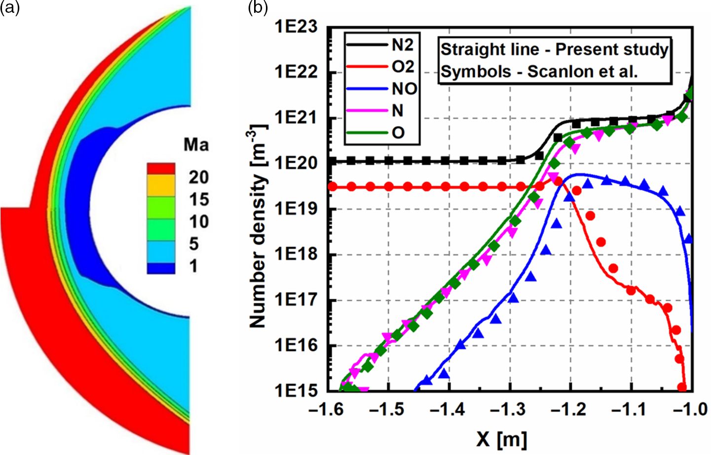
Figure 5. (a) Comparison of overall Mach number contour between published Q–K results by Scanlon et al. [Reference Scanlon52] (lower half) and present simulation results (upper half), (b) Comparison of number density along the stagnation line.
3.2 Verification
The various errors involved in the DSMC technique [Reference Karchani and Ejtehadi53] are thoroughly examined in the present section. The verification studies are typically carried out for cell size, time-step, particles per cell, and number of samples [Reference Guo, Liu and Zhang23, Reference Leite and Santos39]. For grid independency, the flow past BFS for
 $M = 25$
,
$M = 25$
,
 $Kn = 0.05$
, and
$Kn = 0.05$
, and
 $H = 60{\rm{mm}}$
were investigated for different grids, namely, coarse, medium, and fine. The coarse grid consisted of 50% less cells than the medium grid, whereas the fine grid had 50% additional cells. Furthermore, cell ratio (
$H = 60{\rm{mm}}$
were investigated for different grids, namely, coarse, medium, and fine. The coarse grid consisted of 50% less cells than the medium grid, whereas the fine grid had 50% additional cells. Furthermore, cell ratio (
 $\Delta x)$
to mean free path (
$\Delta x)$
to mean free path (
 $\lambda )$
considered was 0.3. Figure 6(a) shows the non-dimensional overall temperature at
$\lambda )$
considered was 0.3. Figure 6(a) shows the non-dimensional overall temperature at
 $X = 59{\rm{mm}}$
for the grids considered. (The dashed purple line in the figures represent the level of the step height
$X = 59{\rm{mm}}$
for the grids considered. (The dashed purple line in the figures represent the level of the step height
 $h = 0.003{\rm{m}}.$
The profile shows a close match for the medium and fine grids. Thus, to reduce the computational time, the medium grid (shown in Fig. 2) was used in all the simulations. Also, the grid was changed as per the mean free path of the corresponding Knudsen number case.
$h = 0.003{\rm{m}}.$
The profile shows a close match for the medium and fine grids. Thus, to reduce the computational time, the medium grid (shown in Fig. 2) was used in all the simulations. Also, the grid was changed as per the mean free path of the corresponding Knudsen number case.
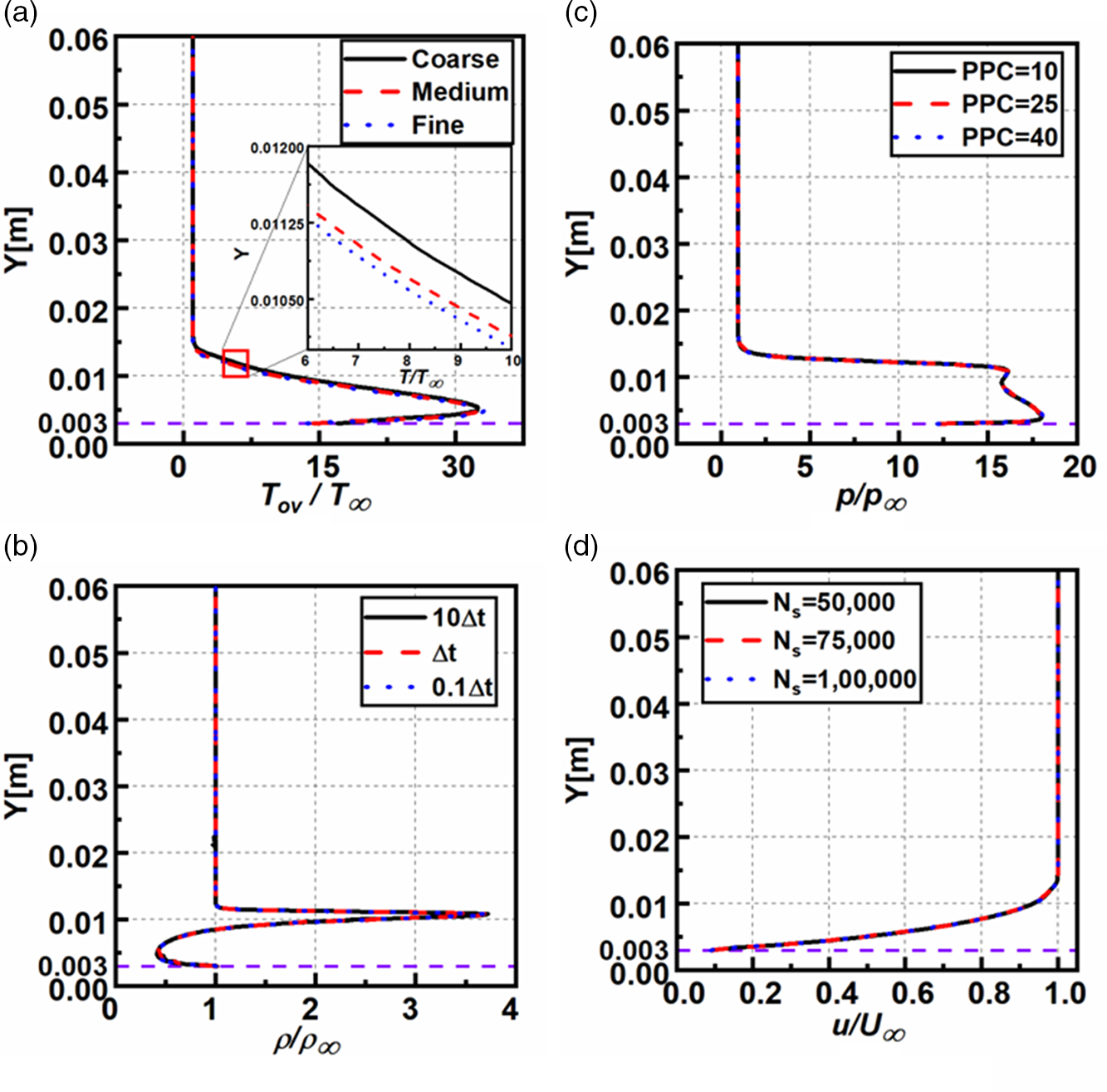
Figure 6. Variation of the non-dimensional (a) overall temperature, (b) density, (c) velocity and (d) pressure in the transverse direction of BFS at
 $X = 120{\rm{mm}}$
for
$X = 120{\rm{mm}}$
for
 $H = 60{\rm{mm}}$
,
$H = 60{\rm{mm}}$
,
 $Kn = 0.05.$
Likewise, for three distinct timesteps, i.e. 10
 $\Delta t$
,
$\Delta t$
,
 $\Delta t,$
and 0.1
$\Delta t,$
and 0.1
 $\Delta t$
, a time-independence evaluation was carried out, with
$\Delta t$
, a time-independence evaluation was carried out, with
 $\Delta t = 2 \times {10^{ - 8}}$
s. For the timesteps considered, the ratio of the time step to the mean collision time are
$\Delta t = 2 \times {10^{ - 8}}$
s. For the timesteps considered, the ratio of the time step to the mean collision time are
 $\Delta t/\Delta {t_{mc}} = 1.17 \times {10^{ - 3}},1.17 \times {10^{ - 4}},1.17 \times {10^{ - 4}}$
, respectively. As a result, all the timesteps assumed were smaller than the mean collision time. Figure 6(b) represents the non-dimensional density for the timesteps, which show a close match for
$\Delta t/\Delta {t_{mc}} = 1.17 \times {10^{ - 3}},1.17 \times {10^{ - 4}},1.17 \times {10^{ - 4}}$
, respectively. As a result, all the timesteps assumed were smaller than the mean collision time. Figure 6(b) represents the non-dimensional density for the timesteps, which show a close match for
 $\Delta t$
and 0.1
$\Delta t$
and 0.1
 $\Delta t$
. This suggests that the selected standard time step is sufficiently small to ensure that computational findings are timestep independent. Thus, a
$\Delta t$
. This suggests that the selected standard time step is sufficiently small to ensure that computational findings are timestep independent. Thus, a
 $\Delta t = 2 \times {10^{ - 8}}$
s was adopted.
$\Delta t = 2 \times {10^{ - 8}}$
s was adopted.
Also, to select an optimum particle per cell (PPC), simulations were performed for three distinct PPC, namely 10, 25, and 40. Figure 6(c) shows the non-dimensional pressure at
 $X = 59{\rm{mm}}$
for the three PPC’s considered, showing an overlapping trend for PPC of 25, 40. Hence a PPC of 25 was adopted.
$X = 59{\rm{mm}}$
for the three PPC’s considered, showing an overlapping trend for PPC of 25, 40. Hence a PPC of 25 was adopted.
A final study was carried out to choose the total number of samples (
 ${N_{\rm{s}}})$
required. Figure 6(d) shows the non-dimensional velocity at
${N_{\rm{s}}})$
required. Figure 6(d) shows the non-dimensional velocity at
 $X = 59{\rm{mm}},$
which overlaps for
$X = 59{\rm{mm}},$
which overlaps for
 ${N_{\rm{s}}} = 75{,}000$
and
${N_{\rm{s}}} = 75{,}000$
and
 ${N_{\rm{s}}} = 1{,}00{,}000.$
Thus
${N_{\rm{s}}} = 1{,}00{,}000.$
Thus
 ${N_{\rm{s}}} = 75{,}000$
was selected. Therefore, the present study’s computational model provides a reasonably good prediction of the cases investigated.
${N_{\rm{s}}} = 75{,}000$
was selected. Therefore, the present study’s computational model provides a reasonably good prediction of the cases investigated.
4.0 Numerical results and discussion
In order to study the rarefaction effects on the flow past BFS, five distinct Knudsen numbers (given in Table 2) in various rarefaction regimes are simulated, and the flow field and surface characteristics are analysed. For all the instances, the free-stream Mach number considered was 25, with a step height of
 $(h = 3{\rm{mm}}$
), and the wall surface
$(h = 3{\rm{mm}}$
), and the wall surface
 $({T_w})$
was maintained at four times the free-stream temperature
$({T_w})$
was maintained at four times the free-stream temperature
 $4{T_\infty }$
. The various flow features are evaluated vertically at four different
$4{T_\infty }$
. The various flow features are evaluated vertically at four different
 $X$
locations, namely
$X$
locations, namely
 $X = 30$
,
$X = 30$
,
 $59$
,
$59$
,
 $61$
, and
$61$
, and
 $120{\rm{mm}}$
, respectively.
$120{\rm{mm}}$
, respectively.
4.1 Flow-field properties
4.1.1 Flow contours
For the case of
 $M = 25$
,
$M = 25$
,
 $Kn = 1.06$
, and
$Kn = 1.06$
, and
 $H = 60{\rm{mm}}$
, the various flow-field contours are shown in Fig. 7(a–d). Figure 7(a) shows the non-dimensional velocity contour depicting the growth of hydrodynamic boundary layer, with lower magnitudes at the wall and higher magnitudes away from it in the central domain. Downstream of the step due to the recirculation region’s formation, the velocity magnitudes are very low. Also, the band of near-wall low velocity extends from the step to the outlet region.
$H = 60{\rm{mm}}$
, the various flow-field contours are shown in Fig. 7(a–d). Figure 7(a) shows the non-dimensional velocity contour depicting the growth of hydrodynamic boundary layer, with lower magnitudes at the wall and higher magnitudes away from it in the central domain. Downstream of the step due to the recirculation region’s formation, the velocity magnitudes are very low. Also, the band of near-wall low velocity extends from the step to the outlet region.

Figure 7. Contours of non-dimensional (a) velocity, (b) density, (c) pressure and (d) overall temperature for
 $H = 60{\rm{mm}}$
,
$H = 60{\rm{mm}}$
,
 ${\rm{M}} = 25$
and
${\rm{M}} = 25$
and
 $Kn = 1.06$
.
$Kn = 1.06$
.
The non-dimensional density contour shown in Fig. 7(b) shows a higher density near the upstream wall and a gradual reduction away from it. The density magnitude is close to one in most of the computational domain. The region close to the step has low density magnitudes due to the recirculation and expansion effects. Furthermore, a high-density magnitude band arises from the upstream surface and traverses towards the top surface, causing a regionalised density rise.
The non-dimensional pressure contour is shown in Fig. 7(c), which attain greater values at the upstream wall and are one order greater than that of the free stream. Due to the minimal influence of the step in the central domain, pressure attains the free-stream value. In the downstream direction, the pressure magnitudes are very low due to the recirculation. Also, the wall pressures are lower than their upstream counterparts, primarily due to the flow expansion.
The non-dimensional overall temperature contour is shown in Fig. 7(d), which follows the pressure contour and depicts higher magnitudes near the wall due to the viscous heating and compressibility phenomena. The band of high temperature at the step height level continues to dissipate the energy farther downstream of the step. Like the pressure contour, the non-dimensional temperature also shows lower magnitudes close to the step; however, these low temperatures are confined to a lower region than the pressure.
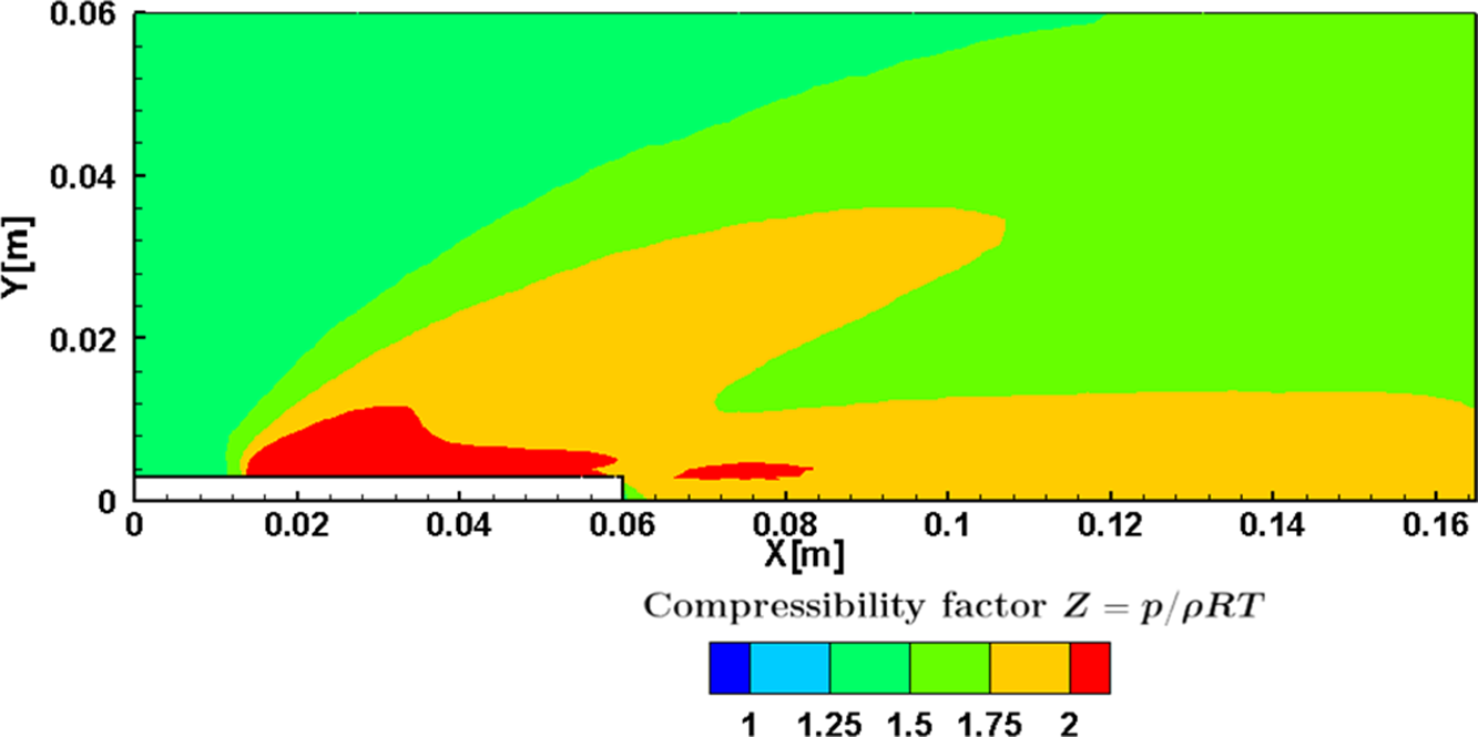
The Compressibility (
 $Z$
) contour is shown in Fig. 8. The compressibility factor shows the departure of the gas from the ideal behaviour and is given by
$Z$
) contour is shown in Fig. 8. The compressibility factor shows the departure of the gas from the ideal behaviour and is given by
 \begin{align}Z = \frac{p}{{\rho RT}}\end{align}
where
 $p$
denotes the pressure,
$p$
denotes the pressure,
 $\rho $
the density,
$\rho $
the density,
 $R$
the gas constant, and
$R$
the gas constant, and
 $T$
is the temperature.
$T$
is the temperature.

Figure 8. Compressibility (
 ${\rm{Z}}$
) contour for
${\rm{Z}}$
) contour for
 $H = 60{\rm{mm}}$
,
$H = 60{\rm{mm}}$
,
 ${\rm{M}} = 25$
and
${\rm{M}} = 25$
and
 $Kn = 1.06$
.
$Kn = 1.06$
.
The regions of higher
 $Z$
magnitudes are witnessed on the upstream surface due to the shear effects. A similar trend is noticed downstream of the step; however, the magnitudes of Z are lower compared to the upstream. In the region close to the step and the center of the domain, the magnitudes of
$Z$
magnitudes are witnessed on the upstream surface due to the shear effects. A similar trend is noticed downstream of the step; however, the magnitudes of Z are lower compared to the upstream. In the region close to the step and the center of the domain, the magnitudes of
 $Z$
are relatively low, depicting equilibrium.
$Z$
are relatively low, depicting equilibrium.
4.1.2 Velocity field
The non-dimensional velocity
 $\left( {u/{U_\infty }} \right)$
distribution for various
$\left( {u/{U_\infty }} \right)$
distribution for various
 $Kn$
at sections
$Kn$
at sections
 $X = 30{\rm{mm}}$
,
$X = 30{\rm{mm}}$
,
 $X = 59{\rm{mm}}$
,
$X = 59{\rm{mm}}$
,
 $X = 61{\rm{mm}},$
and
$X = 61{\rm{mm}},$
and
 $X = 120{\rm{mm}}$
is depicted in Fig. 9(a-d).
$X = 120{\rm{mm}}$
is depicted in Fig. 9(a-d).
 $Y$
represents the perpendicular distance in
$Y$
represents the perpendicular distance in
 $y$
-direction above the BFS surface.
$y$
-direction above the BFS surface.
The profiles at section
 $X = 30{\rm{mm}}$
and
$X = 30{\rm{mm}}$
and
 $X = 59{\rm{mm}}$
are similar, depicting the flow is undisturbed upstream of the step. At Section
$X = 59{\rm{mm}}$
are similar, depicting the flow is undisturbed upstream of the step. At Section
 $X = 61{\rm{mm}}$
, the velocity profiles show negative magnitudes, portraying recirculation; a similar phenomenon was found in Grotowsky and Ballmann’s [Reference Grotowsky and Ballmann54] continuum regime analysis. Interestingly, at section
$X = 61{\rm{mm}}$
, the velocity profiles show negative magnitudes, portraying recirculation; a similar phenomenon was found in Grotowsky and Ballmann’s [Reference Grotowsky and Ballmann54] continuum regime analysis. Interestingly, at section
 $X = 61{\rm{mm}}$
up to the step height, the
$X = 61{\rm{mm}}$
up to the step height, the
 $\left( {u/{U_\infty }} \right)$
profiles overlap for all regimes and show a diverging trend above the step. The profiles close to the outlet at
$\left( {u/{U_\infty }} \right)$
profiles overlap for all regimes and show a diverging trend above the step. The profiles close to the outlet at
 $X = 120{\rm{mm}}$
remain relatively unaffected, like those at the inlet. However, the velocity slip at the wall is significant for all sections, excluding section
$X = 120{\rm{mm}}$
remain relatively unaffected, like those at the inlet. However, the velocity slip at the wall is significant for all sections, excluding section
 $X = 61{\rm{mm}}$
, where the slip is relatively the same for all the regimes [Reference Ejtehadi, Roohi and Esfahani55]. This trend deviates from the traditional continuum results, which show zero velocity at the walls.
$X = 61{\rm{mm}}$
, where the slip is relatively the same for all the regimes [Reference Ejtehadi, Roohi and Esfahani55]. This trend deviates from the traditional continuum results, which show zero velocity at the walls.
The rarefaction effects also reduce the non-dimensional velocity along
 $Y$
. The increase in rarefaction reduces the intermolecular collisions and increases the molecular mean free path. Consequently, the wall effects propagate more into the flow field, reducing the velocity. This is quantified by the boundary layer thickness, another important flow characteristic. Here, the boundary layer thickness (
$Y$
. The increase in rarefaction reduces the intermolecular collisions and increases the molecular mean free path. Consequently, the wall effects propagate more into the flow field, reducing the velocity. This is quantified by the boundary layer thickness, another important flow characteristic. Here, the boundary layer thickness (
 $\delta $
) is extracted considering the point where
$\delta $
) is extracted considering the point where
 $u/{U_\infty } = 0.99$
. For the top surface location considered in the present study, the boundary layer is fully established for different
$u/{U_\infty } = 0.99$
. For the top surface location considered in the present study, the boundary layer is fully established for different
 $Kn$
, except
$Kn$
, except
 $Kn = 21.10,$
which shows a developing trend. For a particular location of
$Kn = 21.10,$
which shows a developing trend. For a particular location of
 $X = 59{\rm{mm}}$
, (
$X = 59{\rm{mm}}$
, (
 $\delta $
) and (
$\delta $
) and (
 $\delta $
/H) are given in Table 6.
$\delta $
/H) are given in Table 6.
Table 6. Thickness of the boundary layer (
 $\delta $
) for various
$\delta $
) for various
 $Kn$
at
$Kn$
at
 $X = 59{\rm{mm}}$

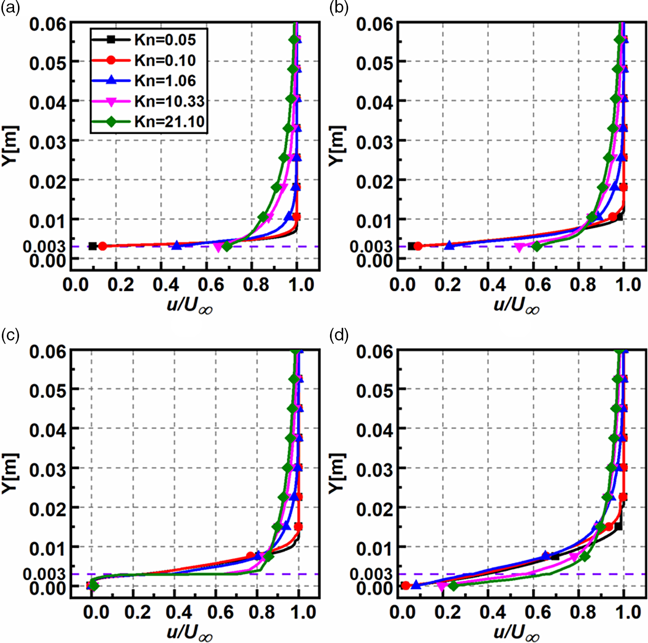
Figure 9. Non-dimensional velocity variation for various
 $Kn$
at (a)
$Kn$
at (a)
 $X = 30{\rm{mm}}$
, (b)
$X = 30{\rm{mm}}$
, (b)
 $X = 59{\rm{mm}}$
, (c)
$X = 59{\rm{mm}}$
, (c)
 $X = 61{\rm{mm}}$
and (d)
$X = 61{\rm{mm}}$
and (d)
 $X = 120{\rm{mm}}$
.
$X = 120{\rm{mm}}$
.
The near-wall velocity (slip) also increases with rarefaction. The profiles for different rarefaction regimes at a given Y location also differ only slightly from each other. At section
 $X = 61{\rm{mm}}$
, magnitudes of
$X = 61{\rm{mm}}$
, magnitudes of
 $\left( {u/{U_\infty }} \right)$
at
$\left( {u/{U_\infty }} \right)$
at
 $Y = 0.03$
are 1.00, 0.99, 0.99, 0.96 and 0.94 for
$Y = 0.03$
are 1.00, 0.99, 0.99, 0.96 and 0.94 for
 $Kn$
0.05, 0.1, 1.06, 10.33 and 21.10, respectively.
$Kn$
0.05, 0.1, 1.06, 10.33 and 21.10, respectively.
The velocity streamlines for different
 $Kn$
are depicted in Fig. 10. It is observed that for all
$Kn$
are depicted in Fig. 10. It is observed that for all
 $Kn$
, a recirculation region exists. Furthermore, streamlines of the free-molecular flow for the case of
$Kn$
, a recirculation region exists. Furthermore, streamlines of the free-molecular flow for the case of
 $Kn = 21.10$
suggests that there exists a secondary smaller recirculation region. The lengths of recirculation for various
$Kn = 21.10$
suggests that there exists a secondary smaller recirculation region. The lengths of recirculation for various
 $Kn$
in is given in Table 7. These lengths are calculated from the corner of the step (i.e. from
$Kn$
in is given in Table 7. These lengths are calculated from the corner of the step (i.e. from
 $X = 60{\rm{mm}}$
) and are denoted by
$X = 60{\rm{mm}}$
) and are denoted by
 ${X_{\rm{L}}}$
and
${X_{\rm{L}}}$
and
 ${Y_{\rm{L}}}$
. These are extracted where the skin friction coefficient
${Y_{\rm{L}}}$
. These are extracted where the skin friction coefficient
 $\left( {{C_f} = 0} \right)$
[Reference Schäfer, Breuer and Durst56, Reference Deepak, Gai and Neely57]. Both
$\left( {{C_f} = 0} \right)$
[Reference Schäfer, Breuer and Durst56, Reference Deepak, Gai and Neely57]. Both
 ${X_{\rm{L}}}$
and
${X_{\rm{L}}}$
and
 ${Y_{\rm{L}}}$
show a diminishing value with
${Y_{\rm{L}}}$
show a diminishing value with
 $Kn$
[Reference Xue and Chen15] (as
$Kn$
[Reference Xue and Chen15] (as
 ${\rm{Re}}$
decreases as seen from Table 2). This behaviour is analogous to the one found in continuum flows for decreasing Reynolds number.
${\rm{Re}}$
decreases as seen from Table 2). This behaviour is analogous to the one found in continuum flows for decreasing Reynolds number.
Table 7. Recirculation lengths for different
 $Kn$
$Kn$
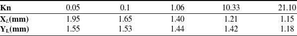
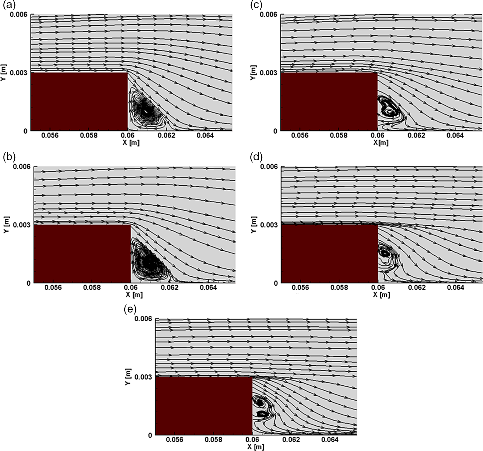
Figure 10. Velocity streamlines for (a)
 $Kn = 0.05$
, (b)
$Kn = 0.05$
, (b)
 $Kn = 0.1$
, (c)
$Kn = 0.1$
, (c)
 $Kn = 1.06$
, (d)
$Kn = 1.06$
, (d)
 $Kn = 10.33$
and (e)
$Kn = 10.33$
and (e)
 $Kn = 21.10$
.
$Kn = 21.10$
.
4.1.3 Velocity slip
The plots of non-dimensional velocity slip
 $\left( {{u_s}/{U_\infty }} \right)$
for different
$\left( {{u_s}/{U_\infty }} \right)$
for different
 $Kn$
on the upper, lower surfaces is shown in Fig. 11. The slip is calculated considering the difference in wall velocity and the fluid close to the wall. It can be extracted by direct sampling of the microscopic particles impacting the wall. It can also be obtained by retrieving the macroscopic flow properties in the cell adjacent to the wall [Reference Balaj, Akhlaghi and Roohi58]; the latter is used in this analysis.
$Kn$
on the upper, lower surfaces is shown in Fig. 11. The slip is calculated considering the difference in wall velocity and the fluid close to the wall. It can be extracted by direct sampling of the microscopic particles impacting the wall. It can also be obtained by retrieving the macroscopic flow properties in the cell adjacent to the wall [Reference Balaj, Akhlaghi and Roohi58]; the latter is used in this analysis.
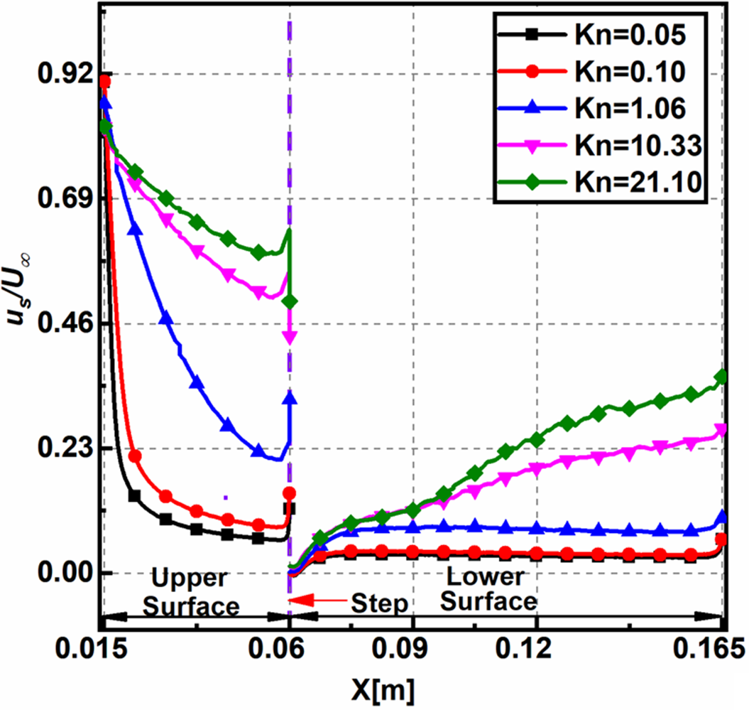
Figure 11. Non-dimensional velocity slip on the upper and lower surfaces for various
 $Kn$
.
$Kn$
.
The velocity slip reduces non-linearly towards the step. Towards the upper surface’s leading edge, the velocity difference between the incoming flow and the wall is large, which leads to a peak in the velocity slip. This decreases downstream as the presence of the wall decelerates the flow. The velocity slip increases along the lower surface downstream of the step, possibly because a larger part of the flow domain gains temperature.
Upstream and downstream of the step, the velocity slip increases with
 $Kn$
due to increased rarefaction effects. For lower
$Kn$
due to increased rarefaction effects. For lower
 $Kn$
, the non-dimensional velocity slip at a given location is less and almost a constant compared to the other cases.
$Kn$
, the non-dimensional velocity slip at a given location is less and almost a constant compared to the other cases.
4.1.4 Pressure field
The non-dimensional pressure
 $\left( {p/{p_\infty }} \right)$
distribution for various
$\left( {p/{p_\infty }} \right)$
distribution for various
 $Kn$
at sections
$Kn$
at sections
 $X = 30{\rm{mm}}$
,
$X = 30{\rm{mm}}$
,
 $X = 59{\rm{mm}}$
,
$X = 59{\rm{mm}}$
,
 $X = 61{\rm{mm}},$
and
$X = 61{\rm{mm}},$
and
 $X = 120{\rm{mm}}$
is presented in Fig. 12(a–d). The non-dimensional pressure behaves similarly in all the sections and increases with increasing the Knudsen number. Also, close to the step, the pressure surpasses the free-stream values by an order of magnitude. There is a considerable variation in the near-wall pressure for different
$X = 120{\rm{mm}}$
is presented in Fig. 12(a–d). The non-dimensional pressure behaves similarly in all the sections and increases with increasing the Knudsen number. Also, close to the step, the pressure surpasses the free-stream values by an order of magnitude. There is a considerable variation in the near-wall pressure for different
 $Kn$
at all the sections, except at
$Kn$
at all the sections, except at
 $X = 61{\rm{mm}}$
, where it is approximately the same. Moreover, the pressure at a specified
$X = 61{\rm{mm}}$
, where it is approximately the same. Moreover, the pressure at a specified
 $X$
attains the free-stream values quicker for
$X$
attains the free-stream values quicker for
 $Kn = 0.05,0.10$
. In section X = 61mm, the pressure in the wake region of the step (for
$Kn = 0.05,0.10$
. In section X = 61mm, the pressure in the wake region of the step (for
 $Y \lt 0.003$
) is close to the free-stream magnitude. Further away from the wall (for
$Y \lt 0.003$
) is close to the free-stream magnitude. Further away from the wall (for
 $Y \gt 0.003)$
, the pressure reaches a peak (owing to the presence of shock layer upstream) and gradually decreases to free-stream value. In
$Y \gt 0.003)$
, the pressure reaches a peak (owing to the presence of shock layer upstream) and gradually decreases to free-stream value. In
 $X = 120{\rm{mm}},$
the pressure profiles behave like those at section
$X = 120{\rm{mm}},$
the pressure profiles behave like those at section
 $X = 61$
mm, but with a marginally lower magnitude. At sections
$X = 61$
mm, but with a marginally lower magnitude. At sections
 $X = 61{\rm{mm}},X = 120{\rm{mm}}$
, the pressure magnitudes decrease due to sudden expansion. Also, due to the compressibility effects of the free-stream flow, there is a pressure surge in all the plots near the step’s face and is highest in the free-molecular regime. For evaluation, in section
$X = 61{\rm{mm}},X = 120{\rm{mm}}$
, the pressure magnitudes decrease due to sudden expansion. Also, due to the compressibility effects of the free-stream flow, there is a pressure surge in all the plots near the step’s face and is highest in the free-molecular regime. For evaluation, in section
 $X = 61{\rm{mm}}$
, the peak pressure ratios are 15.10, 16.01, 36.35, 48.94 and 42.80 for
$X = 61{\rm{mm}}$
, the peak pressure ratios are 15.10, 16.01, 36.35, 48.94 and 42.80 for
 $Kn$
0.05, 0.1, 1.06, 10.33 and 21.10, respectively.
$Kn$
0.05, 0.1, 1.06, 10.33 and 21.10, respectively.
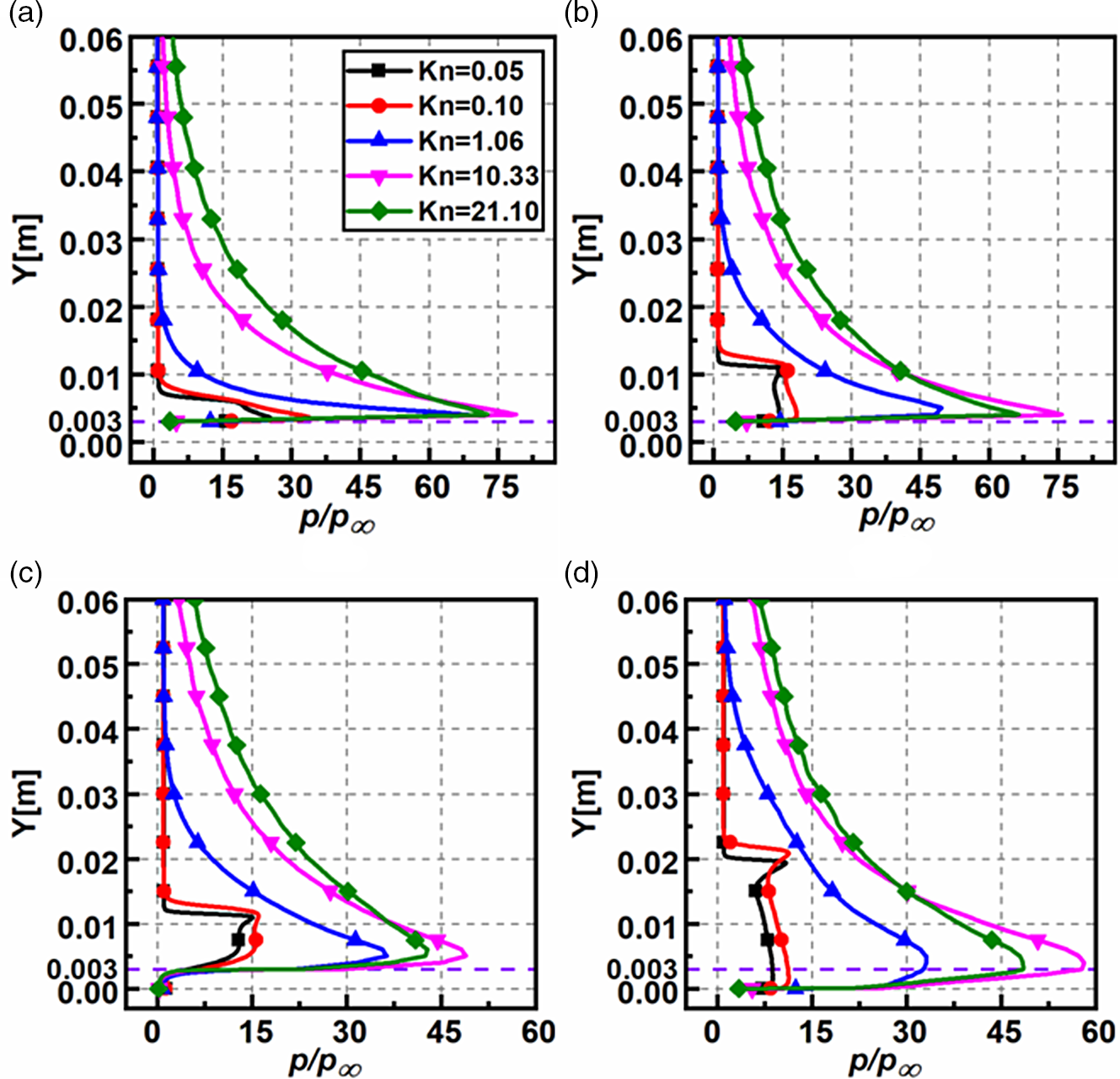
Figure 12. Non-dimensional pressure variation for various
 $Kn$
at (a)
$Kn$
at (a)
 $X = 30{\rm{mm}}$
, (b)
$X = 30{\rm{mm}}$
, (b)
 $X = 59{\rm{mm}}$
, (c)
$X = 59{\rm{mm}}$
, (c)
 $X = 61{\rm{mm}}$
, and (d)
$X = 61{\rm{mm}}$
, and (d)
 $X = 120{\rm{mm}}$
.
$X = 120{\rm{mm}}$
.
4.1.5 Temperature field
The non-dimensional overall temperature
 $\left( {{T_{ov}}/{T_\infty }} \right)$
variation for different
$\left( {{T_{ov}}/{T_\infty }} \right)$
variation for different
 $Kn$
at sections
$Kn$
at sections
 $X = 30{\rm{mm}}$
,
$X = 30{\rm{mm}}$
,
 $X = 59{\rm{mm}}$
,
$X = 59{\rm{mm}}$
,
 $X = 61{\rm{mm}}$
and
$X = 61{\rm{mm}}$
and
 $X = 120{\rm{mm}}$
is described in Fig. 13(a–d). The magnitudes of
$X = 120{\rm{mm}}$
is described in Fig. 13(a–d). The magnitudes of
 $T/{T_\infty }$
increases with
$T/{T_\infty }$
increases with
 $Kn$
at all the sections. Moreover, there is a considerable variation in the near-wall temperature at all the sections, except at
$Kn$
at all the sections. Moreover, there is a considerable variation in the near-wall temperature at all the sections, except at
 $X = 61{\rm{mm}}$
. Because of the substantial flow speed, the viscous heating rates result in a high magnitude of near-wall temperatures. In contrast, at
$X = 61{\rm{mm}}$
. Because of the substantial flow speed, the viscous heating rates result in a high magnitude of near-wall temperatures. In contrast, at
 $X = 61{\rm{mm}}$
, near the vicinity of the step, the temperature near the wall is nearly the same for different
$X = 61{\rm{mm}}$
, near the vicinity of the step, the temperature near the wall is nearly the same for different
 $Kn$
.
$Kn$
.
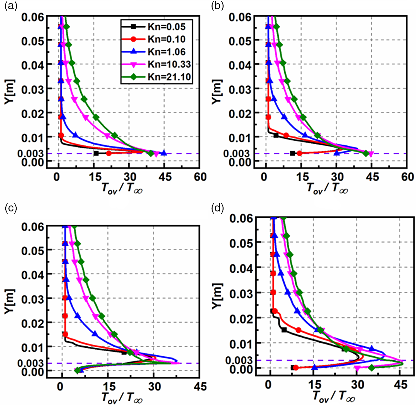
Figure 13. Non-dimensional overall temperature variation for various
 $Kn$
at (a)
$Kn$
at (a)
 $X = 30{\rm{mm}}$
, (b)
$X = 30{\rm{mm}}$
, (b)
 $X = 59{\rm{mm}}$
, (c)
$X = 59{\rm{mm}}$
, (c)
 $X = 61{\rm{mm}}$
, and (d)
$X = 61{\rm{mm}}$
, and (d)
 $X = 120{\rm{mm}}$
.
$X = 120{\rm{mm}}$
.
At the midpoint of the domain, at
 $Y = 0.03$
, the non-dimensional temperature increases with Kn. As
$Y = 0.03$
, the non-dimensional temperature increases with Kn. As
 $Kn$
increase, the molecules’ number density reduces; thus, the viscous heating occurring in the shear layer is dissipated among lesser molecules causing higher magnitudes of non-dimensional temperature [Reference Hong and Asako59]. However, for smaller
$Kn$
increase, the molecules’ number density reduces; thus, the viscous heating occurring in the shear layer is dissipated among lesser molecules causing higher magnitudes of non-dimensional temperature [Reference Hong and Asako59]. However, for smaller
 $Kn$
in the slip and transitional regimes, the number density is several orders higher than the free-molecular regime. Thus, the same viscous heating levels are dispersed among more molecules, causing the overall temperature reduction. For quantitative assessment, at the section
$Kn$
in the slip and transitional regimes, the number density is several orders higher than the free-molecular regime. Thus, the same viscous heating levels are dispersed among more molecules, causing the overall temperature reduction. For quantitative assessment, at the section
 $X = 61{\rm{mm}}$
, the non-dimensional temperature at
$X = 61{\rm{mm}}$
, the non-dimensional temperature at
 $Y = 0.03$
are 0.99, 0.99, 2.31, 7.73 and 9.92 for
$Y = 0.03$
are 0.99, 0.99, 2.31, 7.73 and 9.92 for
 $Kn$
0.05, 0.1, 1.06, 10.33 and 21.10, respectively.
$Kn$
0.05, 0.1, 1.06, 10.33 and 21.10, respectively.
In the transverse direction from the BFS surface, the non-dimensional temperature surges quickly decrease and reach values close to free-stream magnitudes. Again, for quantitative assessment at section
 $X = 61{\rm{mm}}$
, on the top face of the step, the peak temperature ratios are 29.38, 30.69, 37.65, 38.48 and 35.50 for
$X = 61{\rm{mm}}$
, on the top face of the step, the peak temperature ratios are 29.38, 30.69, 37.65, 38.48 and 35.50 for
 $Kn$
0.05, 0.1, 1.06, 10.33 and 21.10, respectively. Thus, the non-dimensional temperature follows an identical pattern in all sections and reasonably shows an increasing trend with
$Kn$
0.05, 0.1, 1.06, 10.33 and 21.10, respectively. Thus, the non-dimensional temperature follows an identical pattern in all sections and reasonably shows an increasing trend with
 $Kn$
.
$Kn$
.
Figure 14(a–d) shows the non-dimensional rotational (
 ${T_R})$
, overall (
${T_R})$
, overall (
 ${T_{OV}})$
, and translational temperature (
${T_{OV}})$
, and translational temperature (
 ${T_T})$
in the perpendicular direction at sections
${T_T})$
in the perpendicular direction at sections
 $X = 30{\rm{mm}}$
,
$X = 30{\rm{mm}}$
,
 $X = 59{\rm{mm}}$
,
$X = 59{\rm{mm}}$
,
 $X = 61{\rm{mm}}$
and
$X = 61{\rm{mm}}$
and
 $X = 120{\rm{mm}}$
for
$X = 120{\rm{mm}}$
for
 $Kn = 0.05,21.10$
. The temperature profiles show a common trend in all sections. However, the magnitudes of the temperature in the free-molecular regime of
$Kn = 0.05,21.10$
. The temperature profiles show a common trend in all sections. However, the magnitudes of the temperature in the free-molecular regime of
 $Kn = 21.10$
is greater than the slip regime of
$Kn = 21.10$
is greater than the slip regime of
 $Kn = 0.05.$
This trend can again be attributed to the number density variation and the dispersion of the viscous heating effects among a lesser number of particles at high
$Kn = 0.05.$
This trend can again be attributed to the number density variation and the dispersion of the viscous heating effects among a lesser number of particles at high
 $Kn$
, as explained earlier. The thermal boundary layer thickness grows as the flow traverses downstream, which can be seen in the peaks near the step height (
$Kn$
, as explained earlier. The thermal boundary layer thickness grows as the flow traverses downstream, which can be seen in the peaks near the step height (
 $Y = 0.003),$
which grows in size. The rotational temperature component shows appreciable variation only in the slip regime, demonstrating that at higher degrees of rarefaction, most of the energy generated due to the wall and shear layer effects manifests itself in the translational and overall temperature components. Also, the change in the rotational component is noticed only at lower
$Y = 0.003),$
which grows in size. The rotational temperature component shows appreciable variation only in the slip regime, demonstrating that at higher degrees of rarefaction, most of the energy generated due to the wall and shear layer effects manifests itself in the translational and overall temperature components. Also, the change in the rotational component is noticed only at lower
 $Kn$
, whereas at higher
$Kn$
, whereas at higher
 $Kn$
the rotational component reasonably remains the same at all sections. Furthermore, the rotational component at the wall increases close to the outlet section of
$Kn$
the rotational component reasonably remains the same at all sections. Furthermore, the rotational component at the wall increases close to the outlet section of
 $X = 120{\rm{mm}}$
when compared to the wake of the step of
$X = 120{\rm{mm}}$
when compared to the wake of the step of
 $X = 61{\rm{mm}}$
.
$X = 61{\rm{mm}}$
.
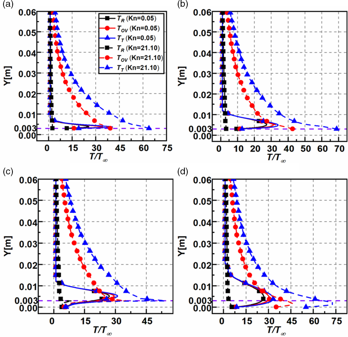
Figure 14. Variation of the non-dimensional rotational, overall, and translational temperature for
 $Kn = 0.05,21.10$
at (a)
$Kn = 0.05,21.10$
at (a)
 $X = 30{\rm{mm}}$
, (b)
$X = 30{\rm{mm}}$
, (b)
 $X = 59{\rm{mm}}$
, (c)
$X = 59{\rm{mm}}$
, (c)
 $X = 61{\rm{mm}}$
and (d)
$X = 61{\rm{mm}}$
and (d)
 $X = 120{\rm{mm}}$
.
$X = 120{\rm{mm}}$
.
4.1.6 Temperature jump
The plots of the non-dimensional temperature jump
 $\left( {{T_j}/{T_\infty }} \right)$
for different
$\left( {{T_j}/{T_\infty }} \right)$
for different
 $Kn$
on the upper, lower surfaces is shown in Fig. 15. The temperature jump is deduced similarly to the velocity slip. For a specified location, the temperature jump shows an increase with
$Kn$
on the upper, lower surfaces is shown in Fig. 15. The temperature jump is deduced similarly to the velocity slip. For a specified location, the temperature jump shows an increase with
 $Kn$
. On the upstream surface for
$Kn$
. On the upstream surface for
 $Kn \le 1.06$
, the temperature jump reaches a peak and decreases towards the step, whereas it continually increases for
$Kn \le 1.06$
, the temperature jump reaches a peak and decreases towards the step, whereas it continually increases for
 $Kn \ge 10.33$
. The wall temperature increase causes a surge in the near-wall fluid temperature, consequently increasing the local mean free path and the rarefaction. This increase in the rarefaction leads to an increase in the temperature jump. The wall shear rates soon decrease downstream of the leading edge and reduce the near-wall temperature and the resulting rarefaction effects. Moreover, the peak value of the temperature jump is about the same for different
$Kn \ge 10.33$
. The wall temperature increase causes a surge in the near-wall fluid temperature, consequently increasing the local mean free path and the rarefaction. This increase in the rarefaction leads to an increase in the temperature jump. The wall shear rates soon decrease downstream of the leading edge and reduce the near-wall temperature and the resulting rarefaction effects. Moreover, the peak value of the temperature jump is about the same for different
 $Kn$
. Additionally, on the lower surface, the temperature jump increases with
$Kn$
. Additionally, on the lower surface, the temperature jump increases with
 $Kn$
like the non-dimensional temperature.
$Kn$
like the non-dimensional temperature.
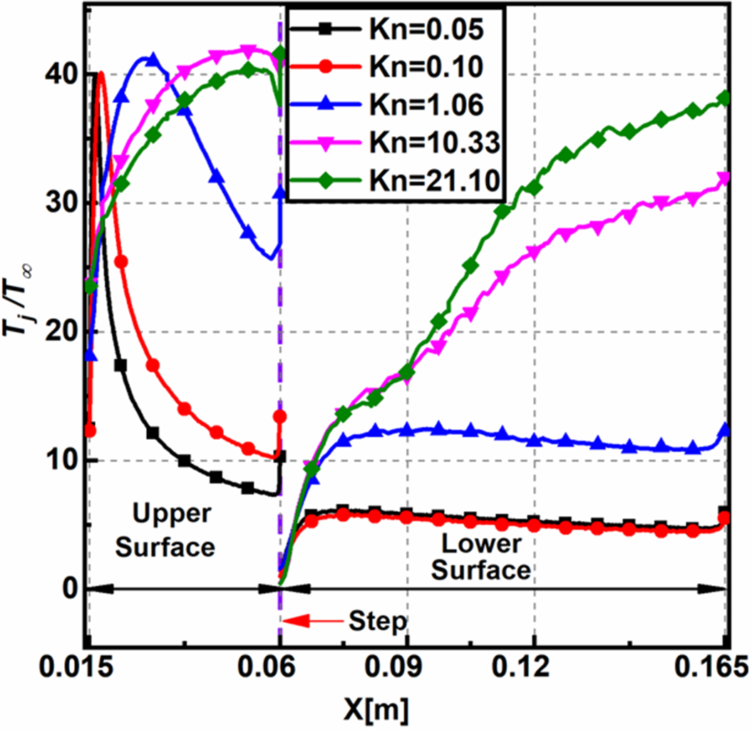
Figure 15. Non-dimensional temperature jump on the upper and lower surfaces for various
 $Kn$
.
$Kn$
.
4.1.7 Density field
The non-dimensional density
 $\left( {\rho /{\rho _\infty }} \right)$
variation for different
$\left( {\rho /{\rho _\infty }} \right)$
variation for different
 $Kn$
at sections
$Kn$
at sections
 $X = 30{\rm{mm}}$
,
$X = 30{\rm{mm}}$
,
 $X = 59{\rm{mm}}$
,
$X = 59{\rm{mm}}$
,
 $X = 61{\rm{mm}}$
and
$X = 61{\rm{mm}}$
and
 $X = 120{\rm{mm}}$
is shown in Fig. 16(a–d). The non-dimensional density varies significantly in the transverse direction, a common feature found in all sections. Another common feature is that the peak density in all sections is observed in the slip regime for
$X = 120{\rm{mm}}$
is shown in Fig. 16(a–d). The non-dimensional density varies significantly in the transverse direction, a common feature found in all sections. Another common feature is that the peak density in all sections is observed in the slip regime for
 $Kn = 0.05$
where it is about four times higher than the free-stream magnitude. At section
$Kn = 0.05$
where it is about four times higher than the free-stream magnitude. At section
 $X = 30{\rm{mm}}$
, the non-dimensional density variation for different
$X = 30{\rm{mm}}$
, the non-dimensional density variation for different
 $Kn$
at a given
$Kn$
at a given
 $Y$
is noticeable, whereas, in other sections, it is not. At section
$Y$
is noticeable, whereas, in other sections, it is not. At section
 $X = 61{\rm{mm}}$
, the densities at the wall are substantially smaller and almost overlap for different
$X = 61{\rm{mm}}$
, the densities at the wall are substantially smaller and almost overlap for different
 $Kn$
. The densities for different
$Kn$
. The densities for different
 $Kn$
are relatively similar all along the face of the step and show a deviating trend after that, signifying that density variation is uninfluenced by a change in
$Kn$
are relatively similar all along the face of the step and show a deviating trend after that, signifying that density variation is uninfluenced by a change in
 $Kn$
in the recirculation region. Far away from the step (
$Kn$
in the recirculation region. Far away from the step (
 $Y \gt 0.003),$
the density decreases beyond the shock wave and eventually tends to the free-stream density. At section
$Y \gt 0.003),$
the density decreases beyond the shock wave and eventually tends to the free-stream density. At section
 $X = 120{\rm{mm}}$
, near the outlet, the density reduces up to
$X = 120{\rm{mm}}$
, near the outlet, the density reduces up to
 $Y = 0.003$
, then experiences a rise attributable to the shock region and, eventually, a reduction to attain the free-stream magnitude. For quantitative evaluation, in section
$Y = 0.003$
, then experiences a rise attributable to the shock region and, eventually, a reduction to attain the free-stream magnitude. For quantitative evaluation, in section
 $X = 61{\rm{mm}}$
, the peak density ratios are 3.751, 2.589, 1.100, 1.172 and 1.170 for
$X = 61{\rm{mm}}$
, the peak density ratios are 3.751, 2.589, 1.100, 1.172 and 1.170 for
 $Kn$
0.05, 0.1, 1.06, 10.33 and 21.10, respectively.
$Kn$
0.05, 0.1, 1.06, 10.33 and 21.10, respectively.
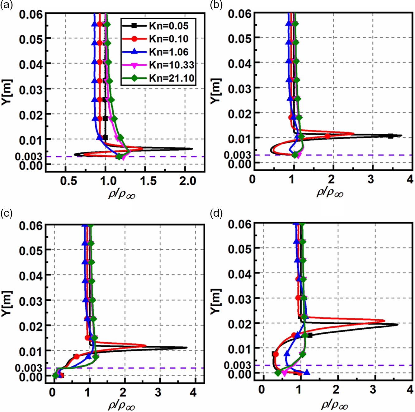
Figure 16. Non-dimensional density variation for various
 $Kn$
at (a)
$Kn$
at (a)
 $X = 30{\rm{mm}}$
, (b)
$X = 30{\rm{mm}}$
, (b)
 $X = 59{\rm{mm}}$
, (c)
$X = 59{\rm{mm}}$
, (c)
 $X = 61{\rm{mm}}$
and (d)
$X = 61{\rm{mm}}$
and (d)
 $X = 120{\rm{mm}}$
.
$X = 120{\rm{mm}}$
.
4.2 Aerodynamic surface properties
4.2.1 Pressure coefficient
The pressure coefficient (
 ${C_p}$
) distribution for various
${C_p}$
) distribution for various
 $Kn$
on the upper and the lower surfaces of the BFS is shown in Fig. 17,
$Kn$
on the upper and the lower surfaces of the BFS is shown in Fig. 17,
 ${C_p}$
is given by
${C_p}$
is given by
 \begin{align}{C_p} = \frac{{{p_w} - {p_\infty }}}{{\frac{1}{2}{\rho _\infty }U_\infty^2}}\end{align}
where,
 ${p_w}$
denotes pressure at the wall,
${p_w}$
denotes pressure at the wall,
 ${U_\infty }$
is the free-stream velocity,
${U_\infty }$
is the free-stream velocity,
 ${p_\infty }$
the free-stream pressure, and
${p_\infty }$
the free-stream pressure, and
 ${\rho _\infty }$
the free-stream density, respectively.
${\rho _\infty }$
the free-stream density, respectively.
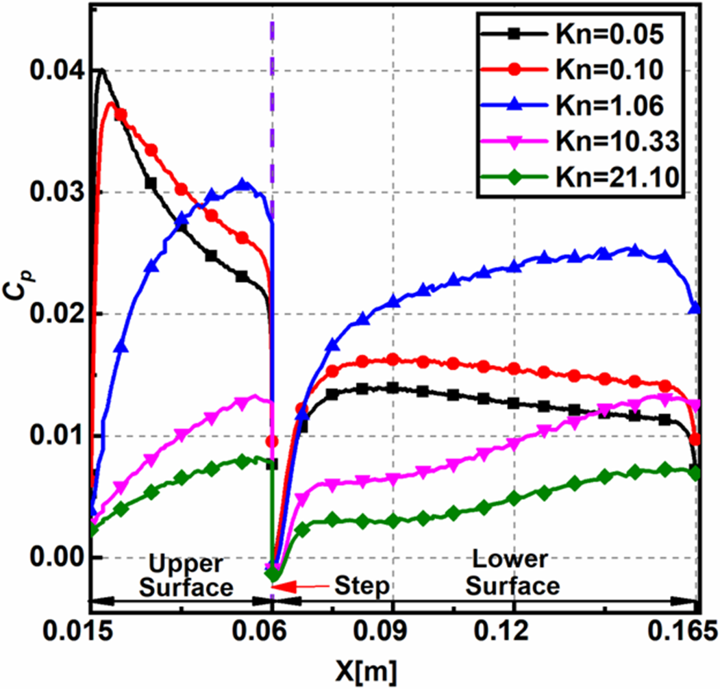
Figure 17. Variation of pressure coefficient
 ${C_p}$
on the upper and lower surfaces for various
${C_p}$
on the upper and lower surfaces for various
 $Kn$
.
$Kn$
.
The profiles adopt similar patterns in the slip regime for
 $Kn = 0.05,0.10,$
and another common trend in the transitional and free-molecular regime for
$Kn = 0.05,0.10,$
and another common trend in the transitional and free-molecular regime for
 $Kn = 1.06,10.33$
and
$Kn = 1.06,10.33$
and
 $21.10$
. The pressure coefficient demonstrates different trends in different rarefaction regimes, the change being observed from
$21.10$
. The pressure coefficient demonstrates different trends in different rarefaction regimes, the change being observed from
 $Kn = 1.06$
onwards. The pressure coefficient
$Kn = 1.06$
onwards. The pressure coefficient
 ${C_p}$
on the upper surface increases along the BFS length; however, there is a sudden peak in the slip regime compared to the transitional and free-molecular regime where the
${C_p}$
on the upper surface increases along the BFS length; however, there is a sudden peak in the slip regime compared to the transitional and free-molecular regime where the
 ${C_p}$
gradually increases. The early peaks in the slip regime can be attributed to the higher near-wall pressure arising from the stagnation pressure rise of the fluid stream (Fig. 12). The peak
${C_p}$
gradually increases. The early peaks in the slip regime can be attributed to the higher near-wall pressure arising from the stagnation pressure rise of the fluid stream (Fig. 12). The peak
 ${C_p}$
on the upper surface is observed at
${C_p}$
on the upper surface is observed at
 $X$
locations of 0.01775, 0.0202, 0.05385, 0.05585 and 0.05595 for
$X$
locations of 0.01775, 0.0202, 0.05385, 0.05585 and 0.05595 for
 $Kn$
0.05, 0.1, 1.06, 10.33 and 21.10, respectively. Also, near the step, the magnitudes of
$Kn$
0.05, 0.1, 1.06, 10.33 and 21.10, respectively. Also, near the step, the magnitudes of
 ${C_p}$
are below zero, owing to recirculation, which reduces the wall pressure below the free-stream value. The
${C_p}$
are below zero, owing to recirculation, which reduces the wall pressure below the free-stream value. The
 ${C_p}$
on the lower surface behaves relatively similar for all cases, where the
${C_p}$
on the lower surface behaves relatively similar for all cases, where the
 ${C_p}$
increases and diminishes towards the outlet in the slip regime, whereas in the transitional and free-molecular regimes the
${C_p}$
increases and diminishes towards the outlet in the slip regime, whereas in the transitional and free-molecular regimes the
 ${C_p}$
shows a gradually increasing trend. Furthermore, for all the cases, the magnitudes
${C_p}$
shows a gradually increasing trend. Furthermore, for all the cases, the magnitudes
 ${C_p}$
near the outlet are greater than zero signifying a net higher near-wall pressure compared to free-stream pressure.
${C_p}$
near the outlet are greater than zero signifying a net higher near-wall pressure compared to free-stream pressure.
4.2.2 Skin friction coefficient
The skin friction coefficient (
 ${C_f}$
) distribution for various
${C_f}$
) distribution for various
 $Kn$
on the upper and the lower surfaces of the BFS is shown in Fig. 18.
$Kn$
on the upper and the lower surfaces of the BFS is shown in Fig. 18.
 ${C_f}$
is given by
${C_f}$
is given by
 \begin{align}{C_f} = \frac{{{\tau _w}}}{{\frac{1}{2}{\rho _\infty } U_\infty^2}}\end{align}
where,
 ${\tau _w}$
denotes the shear stress at the wall,
${\tau _w}$
denotes the shear stress at the wall,
 ${U_\infty }$
is the free-stream velocity, and
${U_\infty }$
is the free-stream velocity, and
 ${\rho _\infty }$
the free-stream density.
${\rho _\infty }$
the free-stream density.

Figure 18. Variation of skin friction coefficient
 ${C_f}$
on the upper and lower surfaces for various
${C_f}$
on the upper and lower surfaces for various
 $Kn$
.
$Kn$
.
Figure 18 shows larger values of
 ${C_f}$
on the upper surface at the inlet owing to the substantial velocity gradients near the wall and progressively shows a decline after that. Also, the
${C_f}$
on the upper surface at the inlet owing to the substantial velocity gradients near the wall and progressively shows a decline after that. Also, the
 ${C_f}$
increases with increase in the Knudsen number. In addition, the magnitudes of
${C_f}$
increases with increase in the Knudsen number. In addition, the magnitudes of
 ${C_f}$
show a significant jump for
${C_f}$
show a significant jump for
 $Kn \ge 10.33.$
For instance, the
$Kn \ge 10.33.$
For instance, the
 ${C_f}$
at inlet almost doubles as
${C_f}$
at inlet almost doubles as
 $Kn$
increases from 10.33 to 21.10. The magnitude of
$Kn$
increases from 10.33 to 21.10. The magnitude of
 ${C_f}$
show negative values close to the step owing to flow recirculation. On the lower surface,
${C_f}$
show negative values close to the step owing to flow recirculation. On the lower surface,
 ${C_f}$
for different
${C_f}$
for different
 $Kn$
rises gradually towards the outlet. The
$Kn$
rises gradually towards the outlet. The
 ${C_f}$
is reasonably same for
${C_f}$
is reasonably same for
 $Kn \le 1.06$
, whereas it gradually increases for other cases. From Equation (2), as
$Kn \le 1.06$
, whereas it gradually increases for other cases. From Equation (2), as
 $Kn$
increases,
$Kn$
increases,
 $Re$
diminishes causing the viscous forces to dominate compared to the inertial forces, which leads to an increase in shear stress and
$Re$
diminishes causing the viscous forces to dominate compared to the inertial forces, which leads to an increase in shear stress and
 ${C_f}$
. At
${C_f}$
. At
 $\left( {X = 60{\rm{mm}}} \right)$
the peak values of
$\left( {X = 60{\rm{mm}}} \right)$
the peak values of
 ${C_f}$
is found to be
${C_f}$
is found to be
 $4.38 \times {10^{ - 4}}$
,
$4.38 \times {10^{ - 4}}$
,
 $3.30 \times {10^{ - 4}}$
,
$3.30 \times {10^{ - 4}}$
,
 $5.60 \times {10^{ - 4}}$
,
$5.60 \times {10^{ - 4}}$
,
 $5.29 \times {10^{ - 3}}$
and
$5.29 \times {10^{ - 3}}$
and
 $9.56 \times {10^{ - 3}}$
for
$9.56 \times {10^{ - 3}}$
for
 $Kn$
0.05, 0.1, 1.06, 10.33 and 21.10, respectively.
$Kn$
0.05, 0.1, 1.06, 10.33 and 21.10, respectively.
4.2.3 Heat transfer coefficient
The heat transfer coefficient (
 ${C_h}$
) distribution for various
${C_h}$
) distribution for various
 $Kn$
on the upper and the lower surfaces of the BFS is shown in Fig. 19.
$Kn$
on the upper and the lower surfaces of the BFS is shown in Fig. 19.
 ${C_h}$
is given by
${C_h}$
is given by
 \begin{align}{C_h} = \frac{{{q_w}}}{{\frac{1}{2}{\rho _\infty }U_\infty^3}}\end{align}
where,
 ${q_w}$
represents the heat flux at the wall,
${q_w}$
represents the heat flux at the wall,
 ${U_\infty }$
is the free-stream velocity, and
${U_\infty }$
is the free-stream velocity, and
 ${\rho _\infty }$
denotes the free-stream density.
${\rho _\infty }$
denotes the free-stream density.
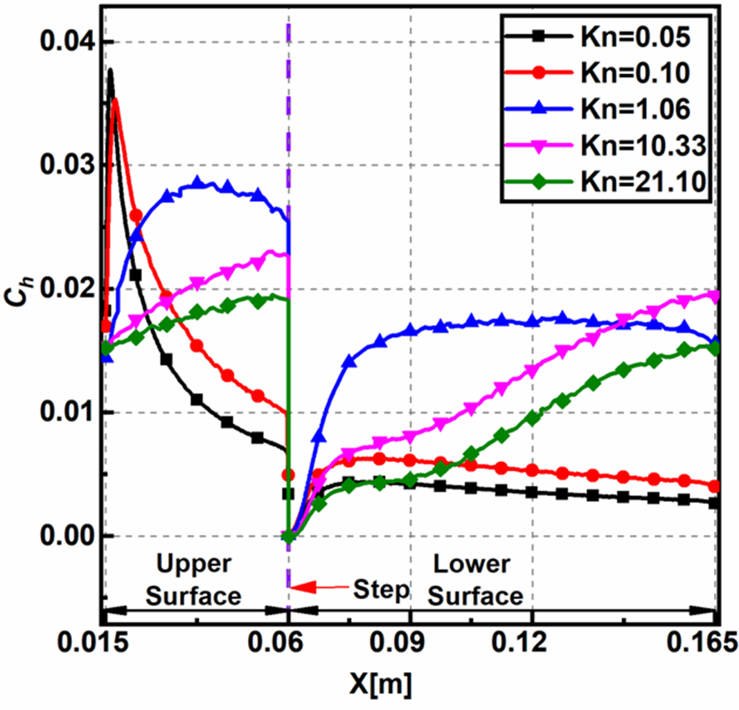
Figure 19. Variation of heat transfer coefficient
 ${C_h}$
on the upper and lower surfaces for various
${C_h}$
on the upper and lower surfaces for various
 $Kn$
.
$Kn$
.
The plots of
 ${C_h}$
and
${C_h}$
and
 ${C_p}$
are similar in appearance. Also, on the upper surface, the profiles are dissimilar for different
${C_p}$
are similar in appearance. Also, on the upper surface, the profiles are dissimilar for different
 $Kn$
. Along the upper surface of the BFS, the heat transfer coefficient
$Kn$
. Along the upper surface of the BFS, the heat transfer coefficient
 ${C_h}$
show a sudden peak for
${C_h}$
show a sudden peak for
 $Kn \le 0.10$
, whereas a gradually increasing trend is observed in the other regimes. The peak
$Kn \le 0.10$
, whereas a gradually increasing trend is observed in the other regimes. The peak
 ${C_h}$
on the upper surface is observed at
${C_h}$
on the upper surface is observed at
 $X$
locations 0.01615, 0.01745, 0.02085, 0.05575 and 0.05595 for
$X$
locations 0.01615, 0.01745, 0.02085, 0.05575 and 0.05595 for
 $Kn$
0.05, 0.1, 1.06, 10.33 and 21.10, respectively. Near the base of the step, because of flow expansion, the temperature reduces, causing a drop in the heat transfer coefficient
$Kn$
0.05, 0.1, 1.06, 10.33 and 21.10, respectively. Near the base of the step, because of flow expansion, the temperature reduces, causing a drop in the heat transfer coefficient
 ${C_h}$
. Along the lower surface the
${C_h}$
. Along the lower surface the
 ${C_h}$
values are relatively constant in the slip regime, showing a gradual increase in the higher rarefaction regimes. As the rarefaction increases, molecules present in the central domain participate in the collisions due to the increased mean free path, causing a rise in the heat transfer coefficient. Also, higher near-wall temperatures owing to viscous heating make the
${C_h}$
values are relatively constant in the slip regime, showing a gradual increase in the higher rarefaction regimes. As the rarefaction increases, molecules present in the central domain participate in the collisions due to the increased mean free path, causing a rise in the heat transfer coefficient. Also, higher near-wall temperatures owing to viscous heating make the
 ${C_h}$
magnitudes positive.
${C_h}$
magnitudes positive.
4.3 Comparison with chemically reacting flows
The flow conditions analysed in the present study are hypersonic, making the system energised, leading to the activation of the vibrational modes of the gas. Therefore, a comparative study is conducted between the reacting and non-reacting flows to demonstrate the differences observed when accounting for the chemical reactions.
The flow-field properties such as velocity, pressure and density showed no marked difference when compared against the non-reacting flows. Hence only the temperature field will be discussed in detail. The non-dimensional temperature contours for different components of the temperature
 $M = 25$
and
$M = 25$
and
 $Kn = 1.06$
are shown in Fig. 20. Figure 20(a) shows that the vibrational component of the temperature, which is relatively lower in magnitude compared to the other components. In the wake of the step, the excitations remain unaffected, and as such, no marked difference is observed in the vibrational temperature. However, towards the outlet, there is a temperature surge.
$Kn = 1.06$
are shown in Fig. 20. Figure 20(a) shows that the vibrational component of the temperature, which is relatively lower in magnitude compared to the other components. In the wake of the step, the excitations remain unaffected, and as such, no marked difference is observed in the vibrational temperature. However, towards the outlet, there is a temperature surge.
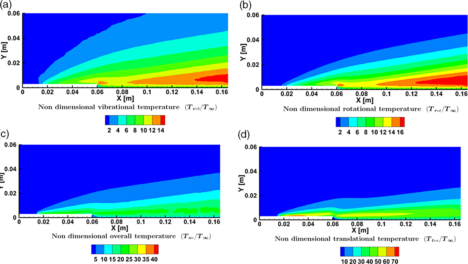
Figure 20. Contours of non-dimensional (a) vibrational, (b) rotational, (c) overall and (d) translational temperature for
 $M = 25$
and
$M = 25$
and
 $Kn = 1.06$
.
$Kn = 1.06$
.
Figure 20(b) shows that the rotational component of the temperature, which is of the same order as that of the vibrational component; however, the magnitudes are marginally higher. Figure 20(c) and (d) show the overall and translational components of the temperature, respectively. The contours show that the translational temperature near the wall is much greater than the temperature imposed at the wall and is of the order of
 ${10^3}$
K. This difference can be attributed to the viscous dissipation effects seen in the shear layer at the step height and near the wall. Similar behaviour is observed for rotational and vibrational temperatures as well. The combined effect is conveyed in the overall temperature contour in Fig. 20(c). Just upstream of the step, the flow begins to expand rapidly. This results in expansion cooling in the vicinity of the step and lower translational and rotational temperature values, as seen from the cold region behind the step. Furthermore, the effects of expansion cooling are also observed downstream near the outlet to reduce the translational temperature. Near the outlet, the high translational temperature in the shear layer downstream of the step reduces due to diffusion, advection, and reduced shear rates. Contrastingly, the rotational and vibrational temperatures are significantly amplified near the outlet due to the non-equilibrium effects, as seen in Fig. 20(a) and (b). The combined effect of this behaviour is reflected in the overall temperature with a relatively uniform temperature variation downstream of the step, where the decreased translational temperature is compensated by the combined effect of increased rotational and vibrational temperature.
${10^3}$
K. This difference can be attributed to the viscous dissipation effects seen in the shear layer at the step height and near the wall. Similar behaviour is observed for rotational and vibrational temperatures as well. The combined effect is conveyed in the overall temperature contour in Fig. 20(c). Just upstream of the step, the flow begins to expand rapidly. This results in expansion cooling in the vicinity of the step and lower translational and rotational temperature values, as seen from the cold region behind the step. Furthermore, the effects of expansion cooling are also observed downstream near the outlet to reduce the translational temperature. Near the outlet, the high translational temperature in the shear layer downstream of the step reduces due to diffusion, advection, and reduced shear rates. Contrastingly, the rotational and vibrational temperatures are significantly amplified near the outlet due to the non-equilibrium effects, as seen in Fig. 20(a) and (b). The combined effect of this behaviour is reflected in the overall temperature with a relatively uniform temperature variation downstream of the step, where the decreased translational temperature is compensated by the combined effect of increased rotational and vibrational temperature.
Figure 21(a–d) compares the temperature profiles normalised with the freestream temperature at different
 $X$
locations. The temperature profiles for both chemically reacting flow as well as non-reacting flow are compared with each other. In all the chemically reacting flow plots, the temperature observed near the wall is an order higher than the imposed wall temperature. Even greater temperature values are observed at the step height in the shear layer due to viscous dissipation. Except for
$X$
locations. The temperature profiles for both chemically reacting flow as well as non-reacting flow are compared with each other. In all the chemically reacting flow plots, the temperature observed near the wall is an order higher than the imposed wall temperature. Even greater temperature values are observed at the step height in the shear layer due to viscous dissipation. Except for
 $X = 61{\rm{mm}}$
, the wall’s temperature ratio increases with rarefaction. At higher
$X = 61{\rm{mm}}$
, the wall’s temperature ratio increases with rarefaction. At higher
 $Kn$
, viscous heat generation is dispersed over fewer molecules, thereby resulting in a more significant temperature increment. At the middle of the flow domain,
$Kn$
, viscous heat generation is dispersed over fewer molecules, thereby resulting in a more significant temperature increment. At the middle of the flow domain,
 $Y = 30{\rm{mm}}$
, the temperature again rises with rarefaction. The general trend observed along the Y direction, away from the wall, is the rapid increase in temperature until it attains a maximum value. It then follows a gradual decrease in the temperature ratio until the ratio equals one.
$Y = 30{\rm{mm}}$
, the temperature again rises with rarefaction. The general trend observed along the Y direction, away from the wall, is the rapid increase in temperature until it attains a maximum value. It then follows a gradual decrease in the temperature ratio until the ratio equals one.
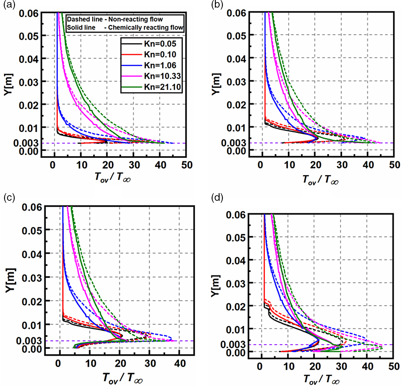
Figure 21. Comparison of the non-dimensional overall temperature for various
 $Kn$
at (a)
$Kn$
at (a)
 $X = 30{\rm{mm}}$
, (b)
$X = 30{\rm{mm}}$
, (b)
 $X = 59{\rm{mm}}$
,(c)
$X = 59{\rm{mm}}$
,(c)
 $X = 61{\rm{mm}}$
and (d)
$X = 61{\rm{mm}}$
and (d)
 $X = 120{\rm{mm}}$
for reacting and non-reacting cases.
$X = 120{\rm{mm}}$
for reacting and non-reacting cases.
When the results are compared with the non-reacting flow, a considerable difference is observed. At
 $X = 30{\rm{mm}}$
the wall temperature ratio values predicted by non-reacting flow, differ with chemically reacting flow by roughly 78%, 109%, 57.2%, 0.49% and −5.7% for
$X = 30{\rm{mm}}$
the wall temperature ratio values predicted by non-reacting flow, differ with chemically reacting flow by roughly 78%, 109%, 57.2%, 0.49% and −5.7% for
 $Kn = 0.05,0.10,1.06,10.33\ {\rm{and}}\ 21.10,$
respectively. Similarly, just upstream of the step at
$Kn = 0.05,0.10,1.06,10.33\ {\rm{and}}\ 21.10,$
respectively. Similarly, just upstream of the step at
 $X = 59{\rm{mm}}$
, the wall temperatures differ by 50.8%, 67.6%, 71%, 16.7% and 5.2% for
$X = 59{\rm{mm}}$
, the wall temperatures differ by 50.8%, 67.6%, 71%, 16.7% and 5.2% for
 $Kn = 0.05,0.10,1.06,10.33\ {\rm{and}}\ 21.10,$
respectively, with respect to the chemically reacting flow. Finally, at
$Kn = 0.05,0.10,1.06,10.33\ {\rm{and}}\ 21.10,$
respectively, with respect to the chemically reacting flow. Finally, at
 $X = 120{\rm{mm}}$
, the error in the wall temperature ratio is between 18% and 19% for all degrees of rarefaction.
$X = 120{\rm{mm}}$
, the error in the wall temperature ratio is between 18% and 19% for all degrees of rarefaction.
At all
 $X$
locations, the free molecular flow shows a good agreement with the results predicted by the non-reacting flow. Furthermore, the maximum temperature in the shear layer also is calculated and the error is measured with the non-reacting flow at various locations. At
$X$
locations, the free molecular flow shows a good agreement with the results predicted by the non-reacting flow. Furthermore, the maximum temperature in the shear layer also is calculated and the error is measured with the non-reacting flow at various locations. At
 $X = 30{\rm{mm}}$
the maximum temperature ratio values predicted by non-reacting flow, differ with chemically reacting flow by roughly 72%, 88.9%, 57.2%, 0.49% and −5.7% for
$X = 30{\rm{mm}}$
the maximum temperature ratio values predicted by non-reacting flow, differ with chemically reacting flow by roughly 72%, 88.9%, 57.2%, 0.49% and −5.7% for
 $Kn = 0.05,0.10,1.06,10.33\ {\rm{and}}\ 21.10,$
respectively. At
$Kn = 0.05,0.10,1.06,10.33\ {\rm{and}}\ 21.10,$
respectively. At
 $X = 59{\rm{mm}}$
, the percentage error is 46.9%, 57.8%, 88.7%, 16.7%, and 5.2% for
$X = 59{\rm{mm}}$
, the percentage error is 46.9%, 57.8%, 88.7%, 16.7%, and 5.2% for
 $Kn = 0.05,0.10,1.06,10.33\ {\rm{and}}\ 21.10$
, respectively. Downstream of the step, the error in the maximum temperature is greater than 40% for all
$Kn = 0.05,0.10,1.06,10.33\ {\rm{and}}\ 21.10$
, respectively. Downstream of the step, the error in the maximum temperature is greater than 40% for all
 $Kn$
at
$Kn$
at
 $X = 61\ {\rm{and}}\ 120{\rm{mm}}.$
5.0 Conclusion
The BFS can be approximated as one of the abnormalities that can occur on the surface of a hypersonic vehicle, the study of which aids in the understanding of the flow dynamics over such vehicles. Thus, this study explores the various loads encountered by a re-entry vehicle passing through different altitudes covering different rarefaction regimes. The DSMC method is used as a numerical tool to conduct the studies. The numerical model is validated with the literature results, and a good agreement is found among them. The investigations were performed to analyse the rarefaction effects on the flow-field and aerodynamic properties. The main conclusions are listed as follows:
-
1. The non-dimensional velocity assumed a non-zero value at the walls, which differs from the traditional continuum approach. Also, the boundary layer thickness increased significantly with rarefaction. Furthermore, the near wall slip also showed an increase with rarefaction.
-
2. Near the downstream of the step, flow recirculation was observed in all regimes. The recirculation lengths decreased with increasing
$Kn$
, which can be attributed to the domination of viscous forces. -
3. The non-dimensional pressure and temperature showed identical behaviour with higher magnitudes near the walls and decreased magnitude away from the wall in the perpendicular direction. Also, the rarefaction effects caused an increase in the magnitudes of both the pressure and temperature in the domain due to viscous dissipation and compressibility effects.
-
4. The different components of the temperature showed similar behaviour with increasing magnitudes with an increase in
$Kn$
. However, the change in the rotational component was noticeable only in the lower rarefaction regimes. -
5. The temperature jump showed a sudden rise along the flow direction, succeeded by a gradual decrease in the slip and transitional regime. In contrast, in the free-molecular regime, the temperature jump showed a gradual increase.
-
6. The non-dimensional density, owing largely to the compressibility of the flow, showed significant changes in the slip regime, whereas minimal variation was found in the other regimes.
-
7. The aerodynamic surface properties
${C_p}$
and
${C_h}$
by and large followed a similar trend, with peak magnitudes located upstream. The skin friction coefficient
${C_f}$
on the other hand, showed a consistent increase with
$Kn$
all along the lower and upper surfaces. Also,
${C_f}$
increased continuously with the distance from the step. -
8. The flow-field properties such as velocity, pressure and density showed no marked difference when compared against the non-reacting flows, whereas considerable variation was observed in the temperature field.


The previous trends give a detailed analysis of the rarefaction effects on the hypersonic flow past BFS and offer valuable insights into the flow characteristics of the cases considered.