


1.0 INTRODUCTION
An aerospike can be used to measure angle-of-attack in the flight of a space vehicle(Reference Hillji and Nelson1), to reduce aerodynamic drag in a satellite launch vehicle(Reference Mehta and Jayachandran2) and to make the stand-off distance for anti-tank projectiles(Reference Mikhail3) and re-entry capsules(Reference d'Humieres and Stollery4). An aerodynamist encounters a variety of aerodynamic design problems associated to flow field characteristics around a spike attached with a blunt-body.
The experimental investigation of the flow-field behaviour around the spiked-blunt body at high speed was initiated in early 1947s. Crawford(Reference Crawford5) experimentally investigated the effects of the spike length on the nature of the flow field for a freestream Mach number 6.8 and Reynolds number range of 0.12 × 10⁶–1.5 × 10⁶, based on the cylinder diameter. According to his experimental investigation, the drag and the heat flux were reduced when the spike was lengthened.
Bogdonoff and Vas(Reference Bogdonoff and Vas6), Wood(Reference Maull7) and Maull(Reference Wood8) experimentally tried to understand the physics of hypersonic flow past spikes attached to blunt bodies. They observed in their experimental studies that a reliable estimation of the aerodynamic effects of the spike can be made in conjunction with flow visualisation techniques. A summary of experimental investigations up to 1966 has been reported in Ref. Reference Chang9 for an axially symmetric model with various spikes shape in the freestream Mach number range of 1.75 ≤ M∞ ≥ 14 and Reynolds number (based on the blunt body diameter) range of 0.85 × 10⁶ ≤ Re ≥ 1.5 × 10⁶.
Kubota(Reference Kubota10) has investigated the overall characteristics of the spiked blunt body configuration at hypersonic Mach numbers. Motoyama et al(Reference Motoyama, Mihara, Miyajima, Watanuki and Kubota11) have experimentally analysed the aerodynamic and heat transfer characteristics of conical, hemispherical, flat-face aerospikes and hemispherical and flat-face discs attached to blunt bodies for a freestream Mach number 7, freestream Reynolds number of 4 × 10⁵/m for L/D = 0.5 and 1.0, and angle-of-attack 0° to 8°. Milicev et al(Reference Milicv, Pavlovic, Ristic and Vitic12) have experimentally investigated the influence of four different types of spikes attached to a hemisphere-cylinder body at Mach number 1.89, Reynolds number 0.38 × 10⁶ based on the cylinder diameter and at an angle-of-attack of 2°. Menezes et al(Reference Menezes, Saravanan, Jagadeesh and Reddy13) carried out experimental investigation to the performance of spiked blunt body in hypersonic speed. Kalimuthu et al(Reference Kalimuthu, Mehta and Rathakrishnan14) have measured aerodynamic forces for hemisphere and flat-face disc spiked blunt body at Mach 6 for L/D = 1.0 and 2.0.
Yamauchi et al(Reference Yamauchi, Fujjii, Tamura and Higashino15) and Mehta(Reference Mehta16) have numerically investigated the flow field around a spiked blunt body at freestream Mach numbers of 2.01, 4.14 and 6.80 for different ratio of L/D. Shoemaker(Reference Shoemaker17), Fujita and Kubota(Reference Fujita and Kubota18), Gerdroodbary et al(Reference Gerdroodbary and Hosseinalipour19) and Mehta(Reference Mehta20) used a numerical approach to solve the compressible Navier-Stokes equations. Their numerical analysis reveals that the reattachment point can be moved backward or removed, which depends on the spike length or the nose configuration. Axisymmetric numerical simulations(Reference Gauer and Paull21) have been performed for different types of spikes attached to a blunt nose cone at Mach numbers of 5.0, 7.0 and 10.0 employing CFD-FASTRAN flow solver. It is found in the numerical simulations that a spike with a disc out-performed the plain pointed spike in terms of drag and aerodynamic heating reduction( Reference Ahmed and Qin 22 , Reference Mehta 23 ). A recent review paper by Ahmed and Qin(Reference Ahmed and Qin24) summarised experimental and numerical investigations on the aerothermodynamics of forward-facing spikes attached to blunt bodies.
The features of the high-speed flow field can be delineated through these experimental and numerical studies. Based on these investigations, a schematic of the flow field around the conical, the hemispherical and the flat-face spiked blunt body at zero angle-of-attack is illustrated Fig. 1. The flow field past a spiked blunt body appears to be very complicated and complex and contains a number of interesting flow phenomena and characteristics, which have yet to be investigated. The high-speed flow over a conical spike shows a formation of a conical shock wave emanating from the tip of the spike as seen in Fig. 1(a). A reattachment shock wave on the blunt body and a separated flow region is formed ahead of the blunt body. In the case of the flat-face and the hemispherical spikes show a formation of a bow shock wave which remains away from the spike, as seen in Figs 1(b) and 1(c). The recirculating region is formed around the root of the spike up to the reattachment point at the shoulder of the hemispherical body. Due to the recirculating region, the pressure at the stagnation region of the blunt body will decrease. However, because of the reattachment of the shear layer on the shoulder of the blunt-body, the pressure near the reattachment point becomes large. Whether the reattachment point can be moved backward or removed, depends on the spike length or the nose configuration. The pressure distribution(Reference Kalimuthu, Mehta and Rathakrishnan25) starts with a negative value at the leading edge, increases up to the point of shear layer attachment, and then exhibits a plateau, which covers a substantial region of the spike length, and finally shows a large increase due to the shear-layer impingement on the blunt body. The spike is characterised by a free shear layer, which is formed as a result of the flow separating from the spike leading edge and reattaching to the blunt body, essentially bridging the spike. The pressure distribution in the spike is relatively constant over most of its length, but shows a rise on the blunt body due to the shear layer attachment(Reference Mehta16). The separating shear layer from the spike leading edge of the flat-face spike attaches to the spike after passing through an expansion fan at the leading-edge corner and a recompression shock at attachment. The attached shear layer then separates near the trailing edge and causes a separation shock before reattaching at the trailing edge prior to undergoing an expansion.
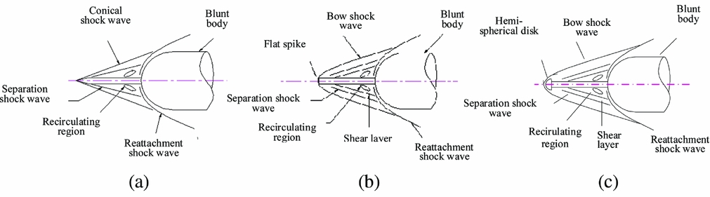
Figure 1. Schematic sketch of the flow field over spike. (a) Conical spike, (b) flat-face spike, (c) hemispherical spike.
This article presents experimental investigation of the fluid flow structure and aerodynamic characteristics of the conical, the hemispherical and the flat-face spiked attached to the blunt bodies at Mach 6 for spike at L/D ratio of range 0.5 to 2.0 (where L is the spike length and D is blunt-body diameter), and angle-of-attack α from 0° to 8° with a 1° step. This article analyses the aerodynamic effects of the shape and geometrical parameters of a spike attached to a blunt body by employing schlieren flow visualisation and measured forces and moment.
2.0 EXPERIMENTAL TECHNIQUES
The experiments were conducted in a blow-down hypersonic wind tunnel at Mach 6. The wind-tunnel system is having a high-pressure air supply, a pebble bed heater, contoured nozzles for obtaining the flow of the required Mach number, a free jet test-section, a fixed geometry diffuser with scoop to collect the nozzle flow and the vacuum system. The facility is equipped with a state-of-the-art instrumentation system and required sensors. The facility is designed to provide a Mach number range of 4 to 8 and Reynolds number 18 × 106. The hypersonic wind tunnel is having jet size of 250mm diameter at the exit of the contour nozzle. Provision is made to enable sliding of the diffuser to scoop back and forth, varying the free jet length from 1.0 to 2.0 times of the nozzle exit diameter to accommodate the desired length of the model. The error for all pressure transducers is within the 0.51% of maximum value of that transducer range. With ±0.51% of error in transducer, dispersions in pressure ratio on the cone surface estimated for Mach 6 freestream and given below:
-
– Uncertainty of P/P∞ at Mach 6 freestream : ±0.084
-
– Aerodynamic force and moments coefficients : ±1.5 %
Wind-tunnel running time is about 30 seconds. Useful data acquisition was about 10 seconds. Transient data acquisition time is 2 seconds before pitching mechanism starts to change the angle-of-attack and 2 seconds after required angle-of-attack achieved.
2.1 Models
Various spike configurations were tested in the present experimental studies. The dimensions of the spiked blunt body considered are shown in Fig. 2. The model is axisymmetric, the main body has a hemisphere-cylinder nose and diameter D = 4.0 × 10⁻² m as shown in Fig. 2. The spike consists of a cylinder stem of diameter 0.1D. Four spikes of length 20mm, 40mm, 60mm and 80mm were designed and fabricated for the configurations considered. The geometrical details of these spikes are shown in Fig. 2. The length L of these spikes was non-dimensionlised with the cylinder diameter, D. Spikes of L/D = 0.5, 1.0, 1.5 and 2.0 were studied for all the configurations. The semi-angle of the cone is 15° as depicted in Fig. 2. The spike configuration utilised the flat-face and the hemispherical as visualised in Fig. 2. The radius of the hemisphere is 0.05D.
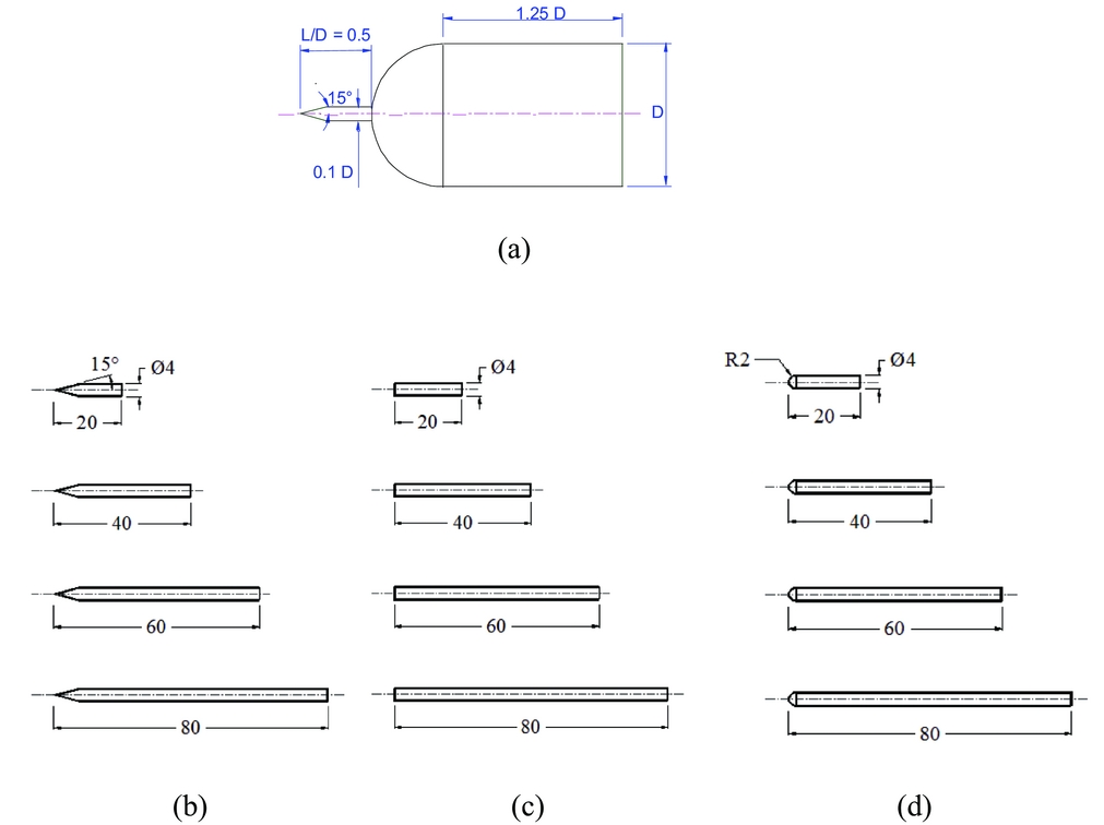
Figure 2. Dimension of spiked-blunt body and conical, flat-face and hemisphere spike. (a) Conical spike with blunt body, (b) conical spike, (c) flat-face spike, (d) hemisphere spike.
2.2 Strain gauge balance
How to use the six-component strain gauge balance is shown in Fig. 3(a). The coefficients of drag, lift and pitching moment are measured for different type of the spike configurations at Mach 6 and α = 0 − 8°. Force measurement data acquisition and processing is essentially done by a DAC in the computer. The computer software can control the functions of the DAC and the acquired data is transferred to the computer during the test through a signal conditioner, amplifier and ADC card. A manual trigger signal from the tunnel control console initiates the data acquisition. This trigger signal also initiates the computer to acquire the data from the total pressure transducer, the angle-of-attack signal from the potentiometer of the pitching mechanism and force measurements data. Data acquired by the ADC in the computer are subsequently processed by separately to get all aerodynamic coefficients.

Figure 3. Strain balance with aerodynamic forces measurements. All dimensions in mm. (a) Strain gauge balance, (b) Strain gauge balance, (c) Sign convention used for forces measurements.
A total of 60 data points was measured and each point was taken, averaging 100 samples. The normal force N1, N2 and the axial force component AF were measured. Total normal force (NF) was derived from the N1 and N2 components. The pitching moment was derived from the N1 and N2 and the moment the arm is the distance between N1 and N2. Figure 3(b) depicts the components of the forces. All the forces are measured with respect to the balance centre and finally transferred to respective spike nose. A schematic sketch showing the notation for the forces and moments are shown in Fig. 3(c). The normal AF and axial NF forces measured using following equations:
 $$\begin{equation}
{C_A} = \frac{{AF}}{{{q_\infty }S}},
\end{equation}$$
$$\begin{equation}
{C_A} = \frac{{AF}}{{{q_\infty }S}},
\end{equation}$$
 $$\begin{equation}
{C_N} = \frac{{NF}}{{{q_\infty }S}},
\end{equation}$$
$$\begin{equation}
{C_N} = \frac{{NF}}{{{q_\infty }S}},
\end{equation}$$
Body axis aerodynamics coefficient like CA and CN is converted to wind axis aerodynamic coefficients of CL and CD with the following relations:
 $$\begin{equation}
{C_L} = {C_A}{\rm{cos}}\alpha {\rm{ \,+\, }}{{\rm{C}}_N}{\rm{sin}}\alpha ,
\end{equation}$$
$$\begin{equation}
{C_L} = {C_A}{\rm{cos}}\alpha {\rm{ \,+\, }}{{\rm{C}}_N}{\rm{sin}}\alpha ,
\end{equation}$$
 $$\begin{equation}
{C_D} = {C_N}{\rm{cos}}\alpha - {{\rm{C}}_A}{\rm{sin}}\alpha ,
\end{equation}$$
$$\begin{equation}
{C_D} = {C_N}{\rm{cos}}\alpha - {{\rm{C}}_A}{\rm{sin}}\alpha ,
\end{equation}$$
and pitching moment and XCP :
 $$\begin{equation}
{C_{PM}} = \frac{{PM}}{{{q_\infty }SL}},
\end{equation}$$
$$\begin{equation}
{C_{PM}} = \frac{{PM}}{{{q_\infty }SL}},
\end{equation}$$
 $$\begin{equation}
{X_{CP}} = \frac{{PM}}{{NF}},
\end{equation}$$
$$\begin{equation}
{X_{CP}} = \frac{{PM}}{{NF}},
\end{equation}$$
where AF, NF and PM is the axial force, normal force and pitching moment, respectively. L is the length of the spike, α is the angle-of-attack, q∞ is the freestream dynamic pressure, S is the reference area based on the cylinder diameter, and XCP is the coefficient of pressure. Positive directions of forces and pitching moment are taken around the nose of the spike. D is taken as reference diameter for the calculation of the aerodynamic coefficients.
3.0 RESULTS AND DISCUSSION
3.1 Flow field visualisation
The schlieren photographs of the flow field around the blunt-body with the conical, hemisphere and flat-face spikes with L/D = 0.5, 1.0, 1.5 and 2.0 are shown in Fig. 4. A conical shock wave can be observed in the case of the conical flat-face. Formation of the bow shock wave is well captured in the case of the hemispherical and the flat-face spike as seen in Fig. 4. We marked other key flow-field features such as compression wave, recirculation zone in the schlieren pictures. The flow fields over the conical, the hemispherical and the flat-face spike are different as can be seen in the schlieren pictures. In the case of the conical spike, the conical shock wave is emanated from the spike tip. The separated shear layer and the recompression shock from the reattachment point on the shoulder of the hemispherical body are visible. Figure 4 depicts the effects of L/D ratio and the angle-of-attack on the flow field. The conical shock wave moves further away from the blunted body and the increase of L/D ratio increases the recirculation zone in the windward side with the angle-of-attack.

Figure 4. Schlieren pictures of conical, flat-face and hemisphere-cap spike at Mach 6. Conical spike (α = 0°), Flat-face spike (α = 0°), Hemisphere-cap spike (α = 0°), Conical spike (α = 8°), Flat-face spike (α = 8°), Hemisphere-cap spike (α = 8°); L/D = 0.5, L/D = 1.0, L/D = 1.5, L/D = 2.0.
A bow shock wave is formed far ahead of the hemispherical cap, as can be observed in Fig. 4. The formation of the bow shock wave is affected by the shape of the spike as well as by the angle-of-attack. The fore-body of the spike is completely enveloped within the recirculation region, which is separated from the inviscid flow within the bow shock wave by a separation shock. The bow shock interacts with the reattachment shock generated by the blunt body. The interaction of the shock wave produced by the hemispherical spike differs significantly with the conical spike. The flow separation on the spike and recirculation zone formed on the blunt body cap depends on shape of the spike. The schlieren pictures explain the cause of the drag reduction due to increase of the separation region over the hemisphere cap type of spike. The normal shock in front of the spike hemisphere cap will reduce the drag as compared without the spike. In the fore-region of the hemisphere cap, the fluid decelerates through the bow shock wave.
The schlieren pictures reveal the flow field behaviour over the spike and also the drag reduction mechanism due to the interaction of the shock waves, which is influenced by the spike configurations as observed in the schlieren pictures.
Based on the schlieren pictures, a schematic diagram of the flow field over the spikes is shown in Fig. 5. The flow fields are different between the hemispherical and the flat-face spikes, as seen in the schematic sketch in Fig. 5. The high-speed flow past the conical spike shows a formation of a conical shock wave emanating from the leading edge of the spike as seen in Fig. 5(a). For high-speed flow past a cone at zero angle-of-attack, the shock wave deflection angle (θ) depends on the M∞ and the semi-cone angle δ.

Figure 5. Schematic diagram of the flow-field over spike. (a) Conical spike, (b) hemispherical cap spike, (c) hemisphere disc spike, (d) flat-face spike, (e) flat-face disc spike.
In the case of the hemisphere spike, a bow shock wave is formed ahead of the spike, as shown in Fig. 5(b) but in the fore region of the hemisphere disc, as seen in Fig. 5(c). The fluid decelerates through the bow shock wave. At the shoulder of the hemispherical disc, the flow turns and expands rapidly, forming a free shear layer that separates the inner recirculating flow region behind the base from the outer flow field. At the shoulder of the hemispherical disc, the flow turns and expands rapidly, and the boundary layer detaches, forming a free shear layer that separates the inner re-circulating flow region behind the base from the outer flow field. The corner expansion over the aero disc process is a modified Prandtl-Meyer(Reference Liepmann and Roshko26) pattern distorted by the presence of the approaching boundary layer. The effects of the subsonic flow on the hemisphere and the flat-face bodies have been investigated by Truitt(Reference Truitt27). The flat-face spike also generates a bow shock wave, which appears practically normal to the body axis(Reference Truitt27), as shown in Fig. 5(d). Since the flow behind the normal shock is always subsonic, simple continuity considerations show that the shock-detachment distance and stagnation-velocity gradient are essentially a function of the density ratio across the shock(Reference Hayer and Probstein28). The flow behind the shock wave is subsonic; the shock is no longer independent of the far-downstream conditions. A change of the spike shape (geometry) in the subsonic region affects the complete flow field up to the shock. For the case of a flat-nosed disc flying at hypersonic speeds as depicted in Fig. 5(e), a detached bow wave is formed in front of the nose which is also having practically normal to the body axis.
3.2 Shock stand-off distance
Figure 5 also represent schematic shock stand-off distance and the location of the sonic line. The shock-detachment distance becomes smaller with increasing density ratio. ProbsteinReference Probstein (29) gives an expression for the shock detachment distance ∆F (Figs 5(b) and 5(c)) with diameter of the flat-disc DS ratio as
 $$\begin{equation}
\frac{{\Delta F}}{{{D_S}}} = 2.8\sqrt {\frac{1}{\varepsilon }}
\end{equation}$$
$$\begin{equation}
\frac{{\Delta F}}{{{D_S}}} = 2.8\sqrt {\frac{1}{\varepsilon }}
\end{equation}$$
The ratio of shock stand-off distance ∆S with hemispherical spike of diameter, DS is
 $$\begin{equation}
\frac{{{\Delta _S}}}{{{D_S}}} = \frac{{2\varepsilon }}{{1 + \sqrt {\frac{{8\varepsilon }}{3}} }},
\end{equation}$$
$$\begin{equation}
\frac{{{\Delta _S}}}{{{D_S}}} = \frac{{2\varepsilon }}{{1 + \sqrt {\frac{{8\varepsilon }}{3}} }},
\end{equation}$$
where ε is the freestream to stagnation density ratio (ρ∞/ρ0) across the normal shock(30). The values of ∆F/DS and ∆S/DS are found to be 0.1898 and 0.1109, respectively. The experimental values of the ratio of shock stand-off to spike cap diameter are taken from schlieren picture, and they are 0.19 and 0.11, which show good agreement with the analytical values. The spherical spike shows the greatest change in velocity gradient as compared to the flat disc(Reference Mehta16,Reference Mehta31) . The shock wave stands in front of the blunt body and forms a region of subsonic flow around the stagnation region.
3.3 Effect of spike geometry on aerodynamic coefficients
3.3.1 Conical spike
The results for conical spike are shown in Figs 6 to 9. It is seen from Fig. 6 that, when there is no spike, in the range of angle-of-attack 0° to 8° the drag coefficient is almost independent of angle-of-attack. When a conical spike of L/D = 0.5 is fixed to the body, the drag coefficient comes down from 0.92 to 0.74. But the angle-of-attack effect on the drag coefficient continues to be insignificant. For spike of L/D = 1.0, the CD at all angles of attack are significantly lower than L/D = 0.5. Also, angle-of-attack influences the CD considerably in the range from 0° to 4°. For L/D = 1.5, the CD comes down drastically for angle-of-attack from 0° to 4°. For angle-of-attack more than 4° even though the drag is much lower than those for the spike of lower L/D, at higher angles of attack the difference between the CD of L/D = 1.0 and 1.5 is much smaller than at lower values of angle-of-attack. When the spike is larger with L/D = 2.0, the drag comes down further, but the difference between L/D = 1.5 and 2.0 becomes insignificant for angles of attack beyond 4°. Therefore, it appears that there is a limiting L/D for the spike, at which the drag reduction obtained is the optimum, in the present range of parameters. The optimum L/D of spike is around 2. A maximum of about 55% reduction in the drag coefficient is achieved for a spike of L/D = 2.0, in the range of angle-of-attack from 0° to 2°.

Figure 6. CD vs angle-of-attack for conical aerospike of different L/D at Mach 6.
When a spike is used at an angle-of-attack, there will be a normal force due to the spike (referred to as lift in the present analysis). At many situations, this is an undesirable force that has to be balanced by some control devices. To quantify the lift force encountered with the spike, the lift coefficient, CL , variation with angle-of-attack for different L/D of conical spike is plotted in Fig. 7. When there is no spike, the basic body experiences a small CL variation with angle-of-attack. The maximum CL is at 8°. For the spike of L/D = 0.5, the variation of CL shows similar trend as the basic body. But at all angles of attack, the magnitude of CL is significantly higher than the basic body CL . These differences monotonically increase with increase of angle-of-attack. For L/D = 1.0, 1.5 and 2.0 the variation of CL with angle-of-attack becomes non-linear. The magnitude of CL increases sharply up to about 4° angle-of-attack, beyond 4° the increase of CL is reduced significantly. The maximum CL is for L/D = 2, at all values of angle-of-attack. Further, for L/D = 1.5 and 2.0, CL becomes independent of angle-of-attack for more than 5°.

Figure 7. CL vs angle-of-attack for conical aerospike of different L/D at Mach 6.
To get an idea about the moment caused by the additional force CL , the pitching moment variations with the angle-of-attack for different L/D is shown in Fig. 8, these pitching moments are about the nose of the spikes. For the basic body, the pitching moment shown in this figure is about the nose of the body. Typical of the body under consideration, the pitching moment of the basic body decreases with increase of angle-of-attack, as seen in this plot. In the present analysis, the nose-up moment is taken as positive and the nose-down moment is taken as negative. As in the case of basic body, for L/D = 0.5 also the pitching moment decreases with increase of angle-of-attack, almost linearly at all levels of angle-of-attack. The CPM for L/D = 0.5 is lower than the basic body CPM . For L/D = 1.0, 1.5 and 2.0, the variation of CPM with angle-of-attack becomes non-linear. Also, the rate of decrease of CPM with increase of angle-of-attack becomes faster with increase of L/D.

Figure 8. CPM vs angle-of-attack for conical aerospike of different L/D at Mach 6.
The centre of the pressure location variation with angle-of-attack is shown in Fig. 9. For the basic body, the XCP moves upstream of the nose with angle-of-attack increase. It is important to note that, in the calculation of XCP , the pitching moment is taken about the nose of the body for the basic body and about the nose of the spike in the case of a basic body with a spike. Therefore, for all cases, the XCP assumes positions upstream of the basic body nose. The ordinate values are from the nose of the body in the upstream direction (conventional notation for these values are supposed to be with a negative sign when the origin is taken at the nose of the basic body).

Figure 9. X cp/L vs angle-of-attack for conical aerospike of different L/D at Mach 6.
It is seen from these results that the XCP is at about 0.9D at angle-of-attack equal to 0°. From angle-of-attack 0° to about 1.5°, the XCP is continuous to be at 0.9D. For angles of attack more than 1.5°, it gradually shifts upstream up to about 5°. For angle-of-attack more than 5°, the XCP becomes almost independent of angle-of-attack. For L/D = 0.5, the centre of pressure shifts downstream up to about angle-of-attack 4° and beyond that it becomes insensitive to the variation of angle-of-attack. For L/D = 1.0, for low values of angle-of-attack 0° to 0.5°, the XCP moves upstream but for all angles of attack beyond 1°, its locations is almost independent of angle-of-attack. Similar is the case for L/D = 1.5 and 2.0. It is important to note that, consideration for compensation of the increase pitching moment is required in order to account the usefulness of the spike in various angle-of-attack situations.
3.3.2 Hemisphere spike
Variation of the CD , CL , CPM and XCP location with angle-of-attack for basic model and model with spike of L/D ratios 0.5, 1.0, 1.5 and 2 are shown in Figs 10 to 13. From Fig. 10, it is seen that, for all L/Ds of the hemisphere spike, the CD is significantly lower than the conical spike at all angles of attack. For the hemisphere spike of L/D = 0.5, the results show that, the CD reduction is only marginal, but the CD level for this length is almost independent of angle-of-attack. For L/D = 1.0, the reduction in CD is appreciably larger than the corresponding conical spike at angles of attack. With the increase of L/D from 1.5 to 2.0, the CD decreases significantly at all angles of attack, compared to the conical spike. For the hemisphere spike, the maximum CD reduction is about 77% at zero angle-of-attack.

Figure 10. CD vs angle-of-attack for hemisphere aerospike of different L/D at Mach 6.
The CL variation with angle-of-attack, shown in Fig. 11, shows that the levels CL for the hemisphere spike is significantly higher than the CL for the conical spike for L/D = 0.5 and 1.0, at all angles of attack. But for L/D = 1.5 and 2.0, the increase in CL compared to conical spike is only marginal.
Figure 11. CL vs angle-of-attack for hemisphere aerospike of different L/D at Mach 6.
The CPM variation with angle-of-attack for the hemisphere spike shown in Fig. 12 reveals that, the CPM for this spike is comparable with that of conical spike at all lengths. However, for L/D = 1.0, the non-linearity of these curves increases marginally compared to the conical spike.

Figure 12. CPM vs angle-of-attack for hemisphere aerospike of different L/D at Mach 6.
The XCP variation with angle-of-attack shown in Fig. 13 shows that the trend is almost similar to that of conical spike. From these results, it is evident that, the hemisphere spike influences the CD , causing considerable reduction compared to the conical spike, whereas its influence on CL , CPM and XCP are almost the same as that of conical spike.

Figure 13. Xcp/L vs angle-of-attack for hemisphere aerospike of different L/D at Mach 6.
3.3.3 Flat-face spike
The CD variation with angle-of-attack shown in Fig. 14 reveals that, for L/D = 1.5 and 2.0, the CD levels for this spike is almost the same as that of hemisphere spike at all angles of attack. Whereas, for L/D = 0.5, the CD level for angles of attack from 0° to 4° decreases noticeably lower than that of hemisphere spike. But, for L/D = 1.0, for angle-of-attack from 0° to 4°, the CD level is larger than that of hemisphere spike.

Figure 14. CD vs angle-of-attack for flat-face aerospike of different L/D at Mach 6.
The CL variation with angle-of-attack, shown in Fig. 15, reveals that the CPM levels for the flat-face spike is almost the same as those of hemisphere spike at all L/Ds and angles of attack.

Figure 15. CL vs angle-of-attack for flat-face aerospike of different L/D at Mach 6.
The CPM variation with angle-of-attack is shown in Fig. 16 shows that the CPM levels for the flat-face spike is almost the same as the conical spike at all angles of attack. The variation of XCP with angle-of-attack of the flat-face spike is also identical to that of the hemisphere spike, as shown in Fig. 17.

Figure 16. CPM vs angle-of-attack for flat-face aerospike of different L/D at Mach 6.
Figure 17. Xcp /L vs angle-of-attack for flat-face aerospike of different L/D at Mach 6.
3.4 Effect of spike length on aerodynamic characteristics
To gain a better understanding about the effect of front geometry of the spikes on the drag, CD variation with angle-of-attack for conical spike, hemisphere spike, flat-face spike, hemisphere disc and flat-face disc are compared in Figs 18 to 21 for L/D = 0.5, 1.0, 1.5 and 2.0, respectively.

Figure 18. CD vs angle-of-attack for different configurations of L/D = 0.5.
For L/D = 0.5, the flat-face disc is the most efficient one resulting in a minimum CD at angle-of-attack. The least efficient ones are the conical and hemisphere spikes, and the flat face spike and hemisphere disc come in between, as seen in Fig. 18. The hemisphere disc and flat-face spike perform almost closer for L/D = 1.0, as shown in Fig. 19, resulting in CD values lower than other configurations at all angles of attack. For this L/D also the least efficient one is the conical spike. For L/D = 1.5, as shown in Fig. 20, the hemisphere disc is the best, resulting in the minimum drag at all angles of attack, compared to other spikes as in the case of lower L/Ds. For this L/D also, the conical spike is the least efficient one. The CD variation with angle-of-attack in Fig. 21 reveals that, for L/D = 2, the performance of the conical spike is the least efficient as in the other cases. From these discussions, it is evident that the CD reduction caused by the spike depends strongly on the spike shape and length.

Figure 19. CD vs angle-of-attack for different configurations of L/D = 1.0.

Figure 20. CD vs angle-of-attack for different configurations of L/D = 1.5.

Figure 21. CD vs angle-of-attack for different configurations of L/D = 2.0.
From these studies, it is found that the spike can serve as an efficient drag-reducing device at hypersonic Mach numbers. The drag on the basic body is strongly influenced by the length-to-diameter ratio, nose shape and the angle-of-attack of the spikes. Among the spikes studied, the most efficient one is the hemispherical spike with L/D = 2.0. This causes a maximum drag reduction of about 77% at 0° angle-of-attack. The above aerodynamic behaviour coincides with the schematic sketches shown in Fig. 5. This spikes essentially shifts the strong detached shock at the nose of the basic body to the nose of the spike, also the detached shock is rendered weak because of the smaller radius of the spike nose. These changes cause a drastic reduction of drag.
4.0 CONCLUSION
Flow observation and 6 degrees of freedom force measurements on the blunt body with a conical, hemispherical cap and flat-face spike are carried out at Mach 6 in a hypersonic wind tunnel. The flow fields show different flow features between the conical spike, the hemispherical cap and the flat-face spiked leading edge. The effects of the spike geometrical parameters as well as the shape on the drag, the lift and the pitching moment are studied experimentally.
In the experimental studies, the aerodynamic forces measured in the presence of the spike attached to the blunt-body for the L/D ratio of 0.5, 1.0, 1.5 and 2.0 and angle-of-attack up to 8° at Mach 6 in the centre's hypersonic wind tunnel. The flow field features captured by the schlieren picture were used to determine the mechanism of the drag reduction. The coefficients of drag, lift and pitching moment were measured for different spike configurations using the six-component strain gauge balance. The influence of the spike shock wave generated from the spike interacts with the reattachment shock were also investigated to understand the cause of drag reduction. The drag coefficient is reduced to 62% for L/D = 1.5 and 78% for L/D = 2.0. Consideration for compensation of increased pitching moment is needed.
The effectiveness of spikes length and aerodynamic characteristics, in the form of a cylindrical rod with conical leading edge, hemispherical, flat-face leading edge with base diameter the same as the diameter of the rod and cylindrical rod with flat-face and hemispherical face discs with their base diameter larger than the rod diameter, attached to a blunt-nosed cylindrical body in reducing the drag has been investigated that will be helpful for the selection of the spiked blunt body configuration.


