


NOMENCLATURE
- A
-
aspect ratio of wing (= span2/wing area)
- b
-
wing span
- c
-
wing chord
- CD
-
total drag coefficient (= D/½ρV2S)
- CDi
-
induced drag coefficient
- CDo
-
profile drag coefficient
- CL
-
lift coefficient (= L/½ρV2S)
- CLo
-
lift coefficient at zero angle-of-attack
- CLα
-
lift curve slope
 $( { = \frac{{\partial {C_L}}}{{\partial \alpha }}} )$
- D
-
total drag of wing (= profile drag + induced drag)
- e
-
span efficiency factor
$[ { = {\scriptsize\raise0.7ex\hbox{$1$} \!
/ \!\lower0.7ex\hbox{${( {1 - \sigma } )}$}}} ]$
- h
-
height of wing above the ground (measured at the quarter chord)
- h AG
-
air gap beneath wing (or end plate)
- h TE
-
height of wing above the ground (measured at the wing trailing edge)
- H 1/30
-
highest of the 30th wave height (sea state description)
- IGE
-
In Ground effect
- K 1
-
constant in the lift curve equation (no end plates) – see Equation (12)
- K 2
-
constant in the induced-drag equation (no end plates) – see Equation (25)
- K 3
-
constant in the induced-drag equation (with end plates) – see Equation (21)
- l
-
depth of end plate
- n
-
exponent in lift curve slope equation – see Equation (12)
- NEP
-
No End Plates
- OGE
-
Out of Ground Effect
- S
-
wing area
- t
-
thickness of wing
- WEP
-
With End Plates
- WIG
-
Wing In Ground effect
- α
-
angle-of-attack of the wing
- ρ
-
air density (= 0.00238 slug/ft3, standard day at sea level)
- σ
-
Prandtl's influence coefficient – see Equation (7)


1.0 INTRODUCTION
The phenomenon of reduced induced drag of wings flying close to the ground (or water) has been known since the early days of flight. There have been many theoretical treatments and experiments made of such operational techniques but little work done on developing analysis techniques suitable for quick assessments of what geometries are best to achieve reduced drag using aerofoil shapes, aspect ratios, end plates, winglets or other devices to lower the induced drag. This paper reviews the original work by Wieselsberger, Prandtl, Prandtl's contemporaries and later researchers to provide an updated consistent set of analyses for use in craft design and to provide a better understanding of the aerodynamic flow and vortex formation around such wings with its impact on lowering induced drag.
2.0 BASIC AERODYNAMIC UNDERPINNINGS
From the original work by Lanchester(Reference Lanchester2) and Prandtl(Reference Prandtl3) on the lifting line theory, it is known that, briefly, the lift and drag of wings can be determined respectively through circulation around the wing and vortices emanating from the wing tips. It has become common practice to describe the result (in coefficient form) in the drag polar expressed as:
 $$\begin{equation}
C_D^{} = {C_{{D_o}}} + \frac{{{C_L}^2}}{{\pi A}}
\end{equation}$$
$$\begin{equation}
C_D^{} = {C_{{D_o}}} + \frac{{{C_L}^2}}{{\pi A}}
\end{equation}$$
In the above equation,
 $$\begin{equation}
{C_D} = \frac{{{\rm{Total\ Drag}}}}{{{\raise0.5ex\hbox{$\scriptstyle 1$} \kern-0.1em/\kern-0.15em \lower0.25ex\hbox{$\scriptstyle 2$}}\rho {V^2}S}},
\end{equation}$$
$$\begin{equation}
{C_D} = \frac{{{\rm{Total\ Drag}}}}{{{\raise0.5ex\hbox{$\scriptstyle 1$} \kern-0.1em/\kern-0.15em \lower0.25ex\hbox{$\scriptstyle 2$}}\rho {V^2}S}},
\end{equation}$$
 $$\begin{equation}
{C_{{D_o}}} = {\text{Profile\ Drag\ Coefficent}},
\end{equation}$$
$$\begin{equation}
{C_{{D_o}}} = {\text{Profile\ Drag\ Coefficent}},
\end{equation}$$
 $$\begin{equation}
{C_L} = \frac{{{\rm{Lift}}}}{{{\raise0.5ex\hbox{$\scriptstyle 1$} \kern-0.1em/\kern-0.15em \lower0.25ex\hbox{$\scriptstyle 2$}}\rho {V^2}S}},
\end{equation}$$
$$\begin{equation}
{C_L} = \frac{{{\rm{Lift}}}}{{{\raise0.5ex\hbox{$\scriptstyle 1$} \kern-0.1em/\kern-0.15em \lower0.25ex\hbox{$\scriptstyle 2$}}\rho {V^2}S}},
\end{equation}$$
 $$\begin{equation}
A = {\rm{Aspect\ Ratio}} = \frac{{{{{\rm{(Span)}}}^{\rm{2}}}}}{{{\rm{Wing\ Area}}}} = \frac{{{b^2}}}{S}
\end{equation}$$
$$\begin{equation}
A = {\rm{Aspect\ Ratio}} = \frac{{{{{\rm{(Span)}}}^{\rm{2}}}}}{{{\rm{Wing\ Area}}}} = \frac{{{b^2}}}{S}
\end{equation}$$
The second term in the drag polar (Equation (1)) is the induced-drag coefficient (CDi ) for wings flying out of ground effect. Prandtl and Wieselsberger(Reference Wieselsberger4) developed the expression for induced drag (CDi ) for wings flying in ground effect to be:
 $$\begin{equation}
{C_{{D_i}}} = \left( {1 - \sigma } \right)\frac{{{C_L}^2}}{{\pi A}}
\end{equation}$$
$$\begin{equation}
{C_{{D_i}}} = \left( {1 - \sigma } \right)\frac{{{C_L}^2}}{{\pi A}}
\end{equation}$$
The modifier for the effect of the proximity of the ground, called the influence coefficient (σ), was developed by Prandtl for inviscid flow using Wieselsberger's theory, as:
 $$\begin{equation}
\sigma = \frac{{1 - 1.32{\raise0.7ex\hbox{$\;h$} \!
/ \!\lower0.7ex\hbox{$b$}}}}{{1.05 + 7.4{\raise0.7ex\hbox{$\;h$} \!
/ \!\lower0.7ex\hbox{$b$}}}}
\end{equation}$$
$$\begin{equation}
\sigma = \frac{{1 - 1.32{\raise0.7ex\hbox{$\;h$} \!
/ \!\lower0.7ex\hbox{$b$}}}}{{1.05 + 7.4{\raise0.7ex\hbox{$\;h$} \!
/ \!\lower0.7ex\hbox{$b$}}}}
\end{equation}$$
The height of the wing (at the quarter chord point) above the ground (h) is referenced to the span (b) of the wing. The lifting-line theory also gave the lift curve slope of a two-dimensional wing flying out of ground effect (in coefficient form) as:
 $$\begin{equation}
{C_L} = \frac{{\partial {C_L}}}{{\partial \alpha }}\alpha
\end{equation}$$
$$\begin{equation}
{C_L} = \frac{{\partial {C_L}}}{{\partial \alpha }}\alpha
\end{equation}$$
In this expression, the two-dimensional lift curve slope is given by:
 $$\begin{equation}
\frac{{\partial {C_L}}}{{\partial \alpha }} = 2\pi
\end{equation}$$
$$\begin{equation}
\frac{{\partial {C_L}}}{{\partial \alpha }} = 2\pi
\end{equation}$$
In this form, the angle-of-attack (α) is measured in radians. For three-dimensional wings, the lift curve slope is modified by the wing aspect ratio, such that:
 $$\begin{equation}
\frac{{\partial {C_L}}}{{\partial \alpha }} = \frac{{2\pi A}}{{A + 2}}
\end{equation}$$
$$\begin{equation}
\frac{{\partial {C_L}}}{{\partial \alpha }} = \frac{{2\pi A}}{{A + 2}}
\end{equation}$$
In 1941, R T Jones(Reference Jones5) at Langley Research Center in Virginia modified this result for better agreement with experimental tests on wings of different plan-form geometries (elliptical, rectangular, etc.) and gave the result for rectangular wings as:
 $$\begin{equation}
\frac{{\partial {C_L}}}{{\partial \alpha }} = \frac{{2\pi A}}{{A + 3}}
\end{equation}$$
$$\begin{equation}
\frac{{\partial {C_L}}}{{\partial \alpha }} = \frac{{2\pi A}}{{A + 3}}
\end{equation}$$
3.0 LIFT CURVE SLOPE OF WINGS IN GROUND EFFECT
There has been no published theory developed for the value of this lift curve slope for wings operating In Ground Effect (IGE), although many experiments have shown that there is a definite effect. If it is postulated that the lift curve slope would vary with the height above the ground and asymptotically approach the Out of Ground Effect (OGE) value at high values of height (usually taken as h/c > 0.5 to 1), then one can write the expression:
 $$\begin{equation}
{\left| {\frac{{\partial {C_L}}}{{\partial \alpha }}} \right|_{{\rm{IGE}}}} = {\left| {\frac{{\partial {C_L}}}{{\partial \alpha }}} \right|_{{\rm{OGE}}}} + \frac{{{K_1}}}{{{{\left( {{\raise0.7ex\hbox{$h$} \!
/ \!\lower0.7ex\hbox{$b$}}} \right)}^n}}}
\end{equation}$$
$$\begin{equation}
{\left| {\frac{{\partial {C_L}}}{{\partial \alpha }}} \right|_{{\rm{IGE}}}} = {\left| {\frac{{\partial {C_L}}}{{\partial \alpha }}} \right|_{{\rm{OGE}}}} + \frac{{{K_1}}}{{{{\left( {{\raise0.7ex\hbox{$h$} \!
/ \!\lower0.7ex\hbox{$b$}}} \right)}^n}}}
\end{equation}$$
The constants (K 1, n) would be determined from experiment. If one uses the R T Jones value for rectangular wings, this becomes:
 $$\begin{equation}
{\left| {\frac{{\partial {C_L}}}{{\partial \alpha }}} \right|_{{\rm{IGE}}}} = \frac{{2\pi A}}{{A + 3}} + \frac{{{K_1}}}{{{{\left( {{\raise0.7ex\hbox{$h$} \!
/ \!\lower0.7ex\hbox{$b$}}} \right)}^n}}}
\end{equation}$$
$$\begin{equation}
{\left| {\frac{{\partial {C_L}}}{{\partial \alpha }}} \right|_{{\rm{IGE}}}} = \frac{{2\pi A}}{{A + 3}} + \frac{{{K_1}}}{{{{\left( {{\raise0.7ex\hbox{$h$} \!
/ \!\lower0.7ex\hbox{$b$}}} \right)}^n}}}
\end{equation}$$
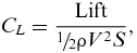
In the 1960s, a considerable amount of experimentation on wings operating in ground effect (and over water) was conducted under controlled tests. Mantle(Reference Mantle1) discusses many of such experiments in detail. From that set of extensive data, three experimenters at NACA, Fink and Lastinger(Reference Fink and Lastinger7) and Carter(Reference Carter8) provided evidence of the effect of the ground (surface) proximity on the lift curve slope for a variety of geometries of different aspect ratios (A) and thickness-to-chord ratios (t/c).
Figure 1 shows some of the results when compared to the above empirical relationship for different thickness chord ratios but with a common aspect ratio, A = 1.
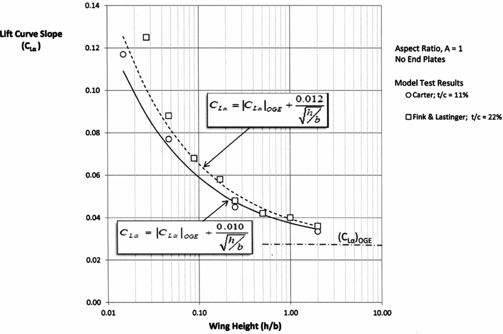
Figure 1. Lift curve slope of wings in ground effect.
The data shows that the “constant” K 1 varies slightly with the thickness of the aerofoil with the values for the two thickness/chord ratios (t/c) tested:
 $$\begin{equation}
{K_1} = 0.012\ {\rm{ for }}\ t/c = 22\% ,
\end{equation}$$
$$\begin{equation}
{K_1} = 0.012\ {\rm{ for }}\ t/c = 22\% ,
\end{equation}$$
 $$\begin{equation}
{K_1} = {\rm{ }}0.010\;{\rm{for}}\;t/c = 11\%
\end{equation}$$
$$\begin{equation}
{K_1} = {\rm{ }}0.010\;{\rm{for}}\;t/c = 11\%
\end{equation}$$
For both sets of data (A = 1), exponent n = 0.5 and the lift curve slope does approach the OGE value asymptotically as the wing moves away from the surface. Note that for A = 1, the parameters h/b and h/c are the same numerically. This point is important when comparing the data on a “chord” basis as used in most theories and on a “span” basis as used here.
In addition, Fink and Lastinger conducted tests for a range of aspect ratios (A = 1–6) but at a constant wing thickness of t/c = 22%. If the postulated solution of Equation (12) is applied to the Fink and Lastinger data but switching to a chord reference, it was found that there were two distinct regions of trends that can be represented for t/c = 22% by:
 $$\begin{equation}
\frac{{\partial {C_L}}}{{\partial \alpha }} = \left| {\frac{{\partial {C_L}}}{{\partial \alpha }}} \right|_{{\rm{OGE}}}^{} + \frac{{0.012}}{{\sqrt {{\raise0.7ex\hbox{$h$} \!
/ \!\lower0.7ex\hbox{$c$}}} }}{\rm{\;for}}\;A \approx 1,
\end{equation}$$
$$\begin{equation}
\frac{{\partial {C_L}}}{{\partial \alpha }} = \left| {\frac{{\partial {C_L}}}{{\partial \alpha }}} \right|_{{\rm{OGE}}}^{} + \frac{{0.012}}{{\sqrt {{\raise0.7ex\hbox{$h$} \!
/ \!\lower0.7ex\hbox{$c$}}} }}{\rm{\;for}}\;A \approx 1,
\end{equation}$$
 $$\begin{equation}
\frac{{\partial {C_L}}}{{\partial \alpha }} = {\left| {\frac{{\partial {C_L}}}{{\partial \alpha }}} \right|_{{\rm{OGE}}}} + \frac{{0.008}}{{{\raise0.7ex\hbox{$h$} \!
/ \!\lower0.7ex\hbox{$c$}}}}\;{\rm{for}}\;A{\rm{ }} \ge 2
\end{equation}$$
$$\begin{equation}
\frac{{\partial {C_L}}}{{\partial \alpha }} = {\left| {\frac{{\partial {C_L}}}{{\partial \alpha }}} \right|_{{\rm{OGE}}}} + \frac{{0.008}}{{{\raise0.7ex\hbox{$h$} \!
/ \!\lower0.7ex\hbox{$c$}}}}\;{\rm{for}}\;A{\rm{ }} \ge 2
\end{equation}$$
This is shown in Fig. 2. The dotted lines are the theoretical results of Prandtl and Jones and the solid lines are the current theory (Equations (16) and (17)).
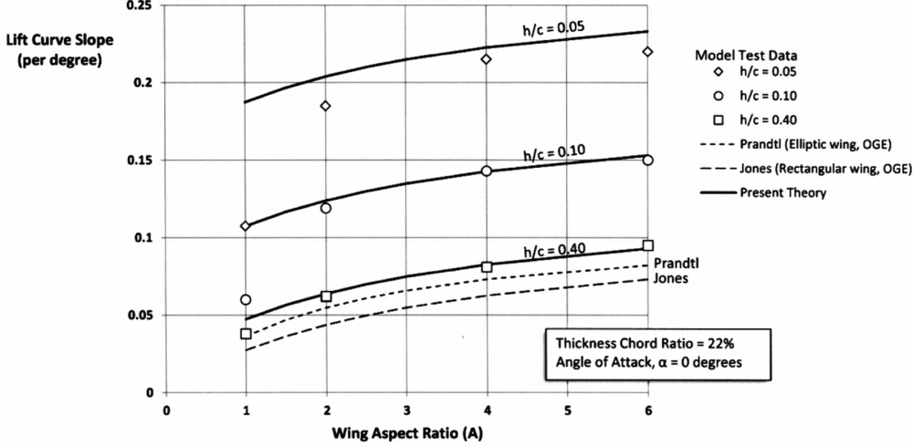
Figure 2. Effect of aspect ratio and height on lift curve slope in ground effect.
Mantle discusses the different flow regimes that affect the aerodynamic characteristics of low-aspect-ratio wings (A ≈ 1) compared to the higher values of aspect ratio (A ≥ 2) due to observed different vortex formation. Pending later experimentation on such low aspect ratio wings in ground effect, the above results give a good representation of the effect of the proximity of the surface to the lift curve slope
 $( {{\raise0.7ex\hbox{${\partial {C_L}}$} \!
/ \!\lower0.7ex\hbox{${\partial \alpha }$}}} )$
of wings before consideration of viscous effects and vortex interaction with the boundary layer at the lower ground clearances.
$( {{\raise0.7ex\hbox{${\partial {C_L}}$} \!
/ \!\lower0.7ex\hbox{${\partial \alpha }$}}} )$
of wings before consideration of viscous effects and vortex interaction with the boundary layer at the lower ground clearances.
4.0 LIFT CURVE SLOPE OF WINGS WITH END PLATES IN GROUND EFFECT
There is limited experimental evidence on the lift curve slope of wings With End Plates (WEP), but the tests conducted over water by Carter for an aspect ratio (A = 1) thin wing (t/c = 11%) provides an opportunity to compare with the same above empirical theory. Figure 3 shows the comparison. The case of wings with No End Plates (NEP) from Fig. 1 has been added for comparison.
Figure 3. Lift curve slope in ground effect of wings with and without end plates.
The data has been taken for the case of zero angle-of-attack (α = 0) such that h/b = hTE/b. The empirical relationships for these two cases can be shown to be:
 $$\begin{equation}
{\rm{No\ End\ Plates}}\left( {{\rm{NEP}}} \right):{\left| {\frac{{\partial {C_L}}}{{\partial \alpha }}} \right|_{{\rm{NEP}}}} = \frac{{2\pi A}}{{A + 3}} + \frac{{0.01}}{{\sqrt {{\raise0.7ex\hbox{$h$} \!
/ \!\lower0.7ex\hbox{$b$}}} }},
\end{equation}$$
$$\begin{equation}
{\rm{No\ End\ Plates}}\left( {{\rm{NEP}}} \right):{\left| {\frac{{\partial {C_L}}}{{\partial \alpha }}} \right|_{{\rm{NEP}}}} = \frac{{2\pi A}}{{A + 3}} + \frac{{0.01}}{{\sqrt {{\raise0.7ex\hbox{$h$} \!
/ \!\lower0.7ex\hbox{$b$}}} }},
\end{equation}$$
 $$\begin{equation}
{\rm{With\ End\ Plates}}\;\left( {{\rm{WEP}}} \right):{\left| {\frac{{\partial {C_L}}}{{\partial \alpha }}} \right|_{{\rm{WEP}}}} = \frac{{2\pi A}}{{A + 3}} + \frac{{0.01}}{{{{\left( {{\raise0.7ex\hbox{$h$} \!
/ \!\lower0.7ex\hbox{$b$}}} \right)}^{{\raise0.5ex\hbox{$\scriptstyle 3$} \kern-0.1em/\kern-0.15em \lower0.25ex\hbox{$\scriptstyle 4$}}}}}}
\end{equation}$$
$$\begin{equation}
{\rm{With\ End\ Plates}}\;\left( {{\rm{WEP}}} \right):{\left| {\frac{{\partial {C_L}}}{{\partial \alpha }}} \right|_{{\rm{WEP}}}} = \frac{{2\pi A}}{{A + 3}} + \frac{{0.01}}{{{{\left( {{\raise0.7ex\hbox{$h$} \!
/ \!\lower0.7ex\hbox{$b$}}} \right)}^{{\raise0.5ex\hbox{$\scriptstyle 3$} \kern-0.1em/\kern-0.15em \lower0.25ex\hbox{$\scriptstyle 4$}}}}}}
\end{equation}$$
It is to be emphasised that these empirical relationships were determined from a limited data set of aerofoil thicknesses, aspect ratios and angles of attack, but they provide a good basis pending later experimentation and confirmation.
5.0 INDUCED DRAG OF WINGS IN GROUND EFFECT WITH END PLATES
It has long been recognised that whether operating in ground effect or out of ground effect, the induced drag of wings can be reduced through various devices such as winglets and most notably by end plates. End plates also helped offset adverse effects of short span on induced drag. Figure 4 shows the configuration used by Carter in his tests over water in the NACA Langley Tow Tank.

Figure 4. WIG model with end plates in NACA tests.
While not detailed in this paper, Mantle(Reference Mantle1) compared these results with the NACA tests of wings With End Plates (WEP) Reference Carter(8) and found that similar effects on lift curve slope and induced drag occurred. The two key results for wings with end plates are:
 $$\begin{equation}
{\left| {\frac{{\partial {C_L}}}{{\partial \alpha }}} \right|_{{\rm{WEP}}}} = \frac{{2\pi A}}{{A + 3}} + \frac{{0.01}}{{{{\left( {{\raise0.7ex\hbox{${{h_{TE}}}$} \!
/ \!\lower0.7ex\hbox{$b$}}} \right)}^{{\raise0.5ex\hbox{$\scriptstyle 3$} \kern-0.1em/\kern-0.15em \lower0.25ex\hbox{$\scriptstyle 4$}}}}}},
\end{equation}$$
$$\begin{equation}
{\left| {\frac{{\partial {C_L}}}{{\partial \alpha }}} \right|_{{\rm{WEP}}}} = \frac{{2\pi A}}{{A + 3}} + \frac{{0.01}}{{{{\left( {{\raise0.7ex\hbox{${{h_{TE}}}$} \!
/ \!\lower0.7ex\hbox{$b$}}} \right)}^{{\raise0.5ex\hbox{$\scriptstyle 3$} \kern-0.1em/\kern-0.15em \lower0.25ex\hbox{$\scriptstyle 4$}}}}}},
\end{equation}$$
 $$\begin{equation}
{\left| {{C_{Di}}} \right|_{{{\rm{WEP}}}}} = {K_3}f\left( {{h_{AG}},h} \right)\frac {C_L^2}{\pi A}
\end{equation}$$
$$\begin{equation}
{\left| {{C_{Di}}} \right|_{{{\rm{WEP}}}}} = {K_3}f\left( {{h_{AG}},h} \right)\frac {C_L^2}{\pi A}
\end{equation}$$
In Equation (21), the constant K 3 = 0.90 gives best fit with the experimental data and the function f(hAG , h) is as given later in Equation (24).
Carter provided complete data on the lift, drag, lift-drag ratio, heights above the ground, etc., on the experiments with various geometric configurations, but it was not until 1970 that a theoretical approach placed some of those parameters on an analytical basis when Ashill(Reference Ashill9) published his theoretical treatment of Wings operating In Ground effect (WIG) with end plates. Later researchers(Reference Kida and Miyai10,Reference Shigenori and Yashiro11) provided similar theories to Ashill but did not provide any experimental confirmation; hence, the focus here is on Ashill's theory and test results. Figure 5 shows the basic geometry. An important distinction between the Carter end plates and those studied by Ashill is that all Carter end plates were constructed with the end plate ending flush with the Trailing Edge (TE) (see Fig. 4). As shown in Fig. 5, Ashill studied end plates that had depths (l/b) that were independent of the height of the TE (hTE/b) and were not flush with the wing TE. This difference has important ramifications on the vortex formation that hampers direct comparison of the Carter and Ashill results.
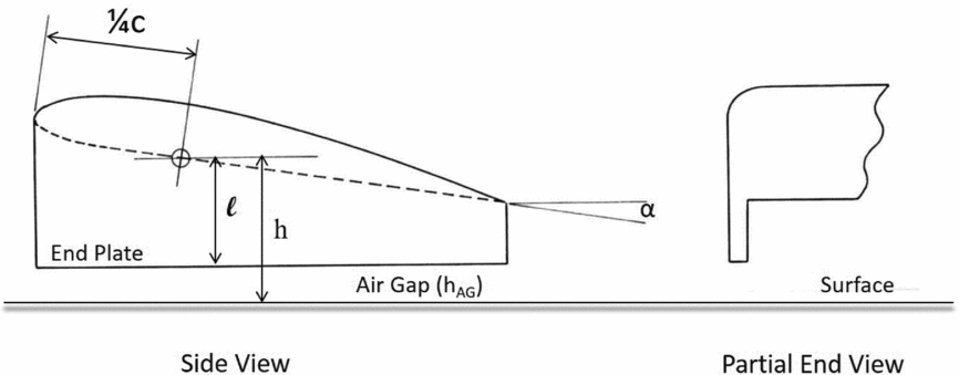
Figure 5. Wing in ground effect with end plates.
In the Ashill treatment, the height of the wing (h) is measured at the quarter chord point and is given by:
 $$\begin{equation}
\frac{h}{b} = \frac{{{h_{TE}}}}{b} + {\raise0.7ex\hbox{$3$} \!
/ \!\lower0.7ex\hbox{$4$}}\frac{{\sin \alpha }}{A}
\end{equation}$$
$$\begin{equation}
\frac{h}{b} = \frac{{{h_{TE}}}}{b} + {\raise0.7ex\hbox{$3$} \!
/ \!\lower0.7ex\hbox{$4$}}\frac{{\sin \alpha }}{A}
\end{equation}$$
In this expression, (hTE ) is the height of the wing at the TE, (b) is the wing span, (α) is the angle-of-attack and (A) is the aspect ratio. The air gap (hAG ) beneath the end plate is related to wing height (h) and the depth of the end plate (l) by:
 $$\begin{equation}
\frac{{{h_{AG}}}}{b} = \frac{{h - l}}{b}
\end{equation}$$
$$\begin{equation}
\frac{{{h_{AG}}}}{b} = \frac{{h - l}}{b}
\end{equation}$$
Ashill presented his results as shown in Fig. 6. The theory by Ashill is complex and does not give specific details on the key geometric factors called out here, and the results are expressed in graphical form without closed-form analytical expressions suitable for design use.
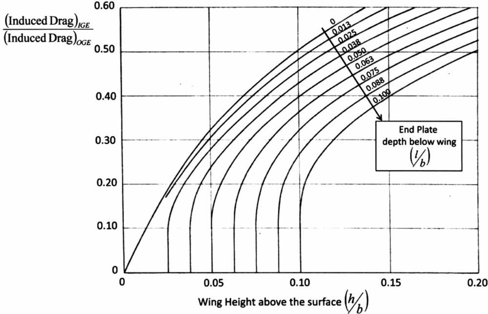
Figure 6. Ashill theory for WIG with end plates.
It is possible to extract some key results, however, through the use of a cross plot of Fig. 6 that reveals the air gap (hAG/b) explicitly, which has been constructed and shown in Fig. 7. The cross plot (dotted lines) allow explicit values of (h/b, l/b and hAG/b) to be determined as related to the reduction of induced drag expressed as a ratio (1 – σ) of the induced drag In Ground Effect (IGE) to the induced drag Out of Ground Effect (OGE). Included in Fig. 7 is the lower bound of applicability of the inviscid theory as put forward by Prandtl and Wieselsberger due to viscous effects and the boundary layer. The end result of the cross plot was that the complex representation of Ashill's graphical solution for induced drag theory for wings in ground effect can now be augmented by a simpler and closed form equation containing direct and measurable geometric features of a wing With End Plates (WEP).
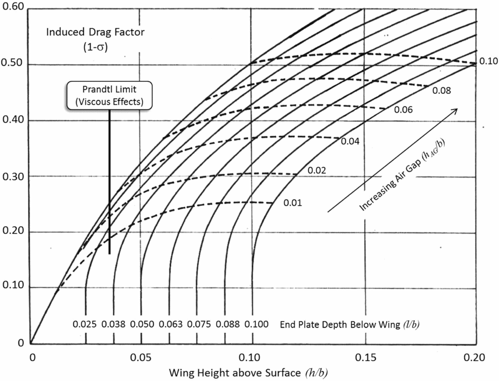
Figure 7. Cross plot of theory to show effect of air gap on induced drag.
This empirical equation for the cross plot is determined to be:
 $$\begin{equation}
{\left( {1 - \sigma } \right)_{{\rm{WEP}}}} = 1.5\left( {\frac{{{h_{AG}}}}{b}} \right) + 5\left( {\frac{h}{b}} \right) - \frac{{10}}{{{{\left( {{\raise0.7ex\hbox{${{h_{AG}}}$} \!
/ \!\lower0.7ex\hbox{$b$}}} \right)}^{{\raise0.5ex\hbox{$\scriptstyle 1$} \kern-0.1em/\kern-0.15em \lower0.25ex\hbox{$\scriptstyle 5$}}}}}}{\left( {\frac{h}{b}} \right)^2}
\end{equation}$$
$$\begin{equation}
{\left( {1 - \sigma } \right)_{{\rm{WEP}}}} = 1.5\left( {\frac{{{h_{AG}}}}{b}} \right) + 5\left( {\frac{h}{b}} \right) - \frac{{10}}{{{{\left( {{\raise0.7ex\hbox{${{h_{AG}}}$} \!
/ \!\lower0.7ex\hbox{$b$}}} \right)}^{{\raise0.5ex\hbox{$\scriptstyle 1$} \kern-0.1em/\kern-0.15em \lower0.25ex\hbox{$\scriptstyle 5$}}}}}}{\left( {\frac{h}{b}} \right)^2}
\end{equation}$$
While the numerical results of the Ashill theory do not show the effect of air gap (hAG ) on induced drag explicitly, it can now be determined using Fig. 7 and Equation (24).
It now becomes a simple matter to express Figs 6 and 7 in a more tractable form showing the key geometric properties and the effect on the induced drag. This is shown in Fig. 8.
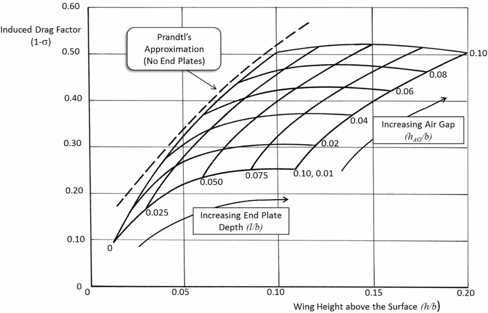
Figure 8. Induced drag of WIG with and without end plates.
Included in Fig. 8 is the Prandtl theory for the induced drag factor (1 – σ) for the case of No End Plates (NEP) (see Equation (7)). Note that over the range of height values deemed valid for inviscid flow by Prandtl, the curve by Ashill for NEP (l/b = 0) closely approximates the results of Prandtl.
6.0 COMPARISON OF THEORY AND EXPERIMENT
Ashill conducted some experiments with wings both with and without end plates in the College of Aeronautics (Cranfield, UK) wind tunnel. The wing was a Clark Y aerofoil section (t/c = 11½%) and aspect ratio (A = 2). Figures 9 and 10 show the results for the wing without end plates (NEP) for two heights above the ground (h/b = 0.125 and 0.083). Included in the two charts are the theoretical results by Prandtl and Ashill compared to the test results by Ashill.
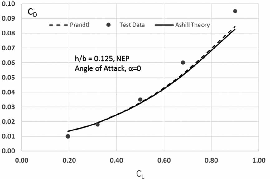
Figure 9. Drag polar at h/b = 0.125 (NEP) (A = 2).
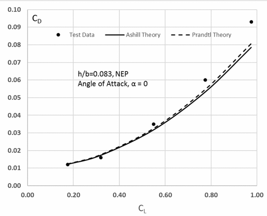
Figure 10. Drag polar at h/b = 0.083 (NEP) (A = 2).
At first glance, it can be thought that the inviscid theory gives a reasonable agreement to the experimental results. The Ashill results shown are taken from his theory for the case of zero angle-of-attack (α = 0). The curves (not shown) for α > 0 from this theory do not match the experimental results as well. Ashill suggests that this is due to the change in vortex formation as the angle-of-attack (α) increases. Resolution of this point must await more systematic testing under controlled test conditions.
The agreement of the Ashill theory with experiments when end plates are added to the wings is shown in Figs 11 and 12 for the same two heights as for Figs 9 and 10, except that now end plates have been added of the same end plate depth (l/b = 0.045) resulting in two different air gaps beneath the end plates (hAG/b = 0.0835 and 0.042, respectively).
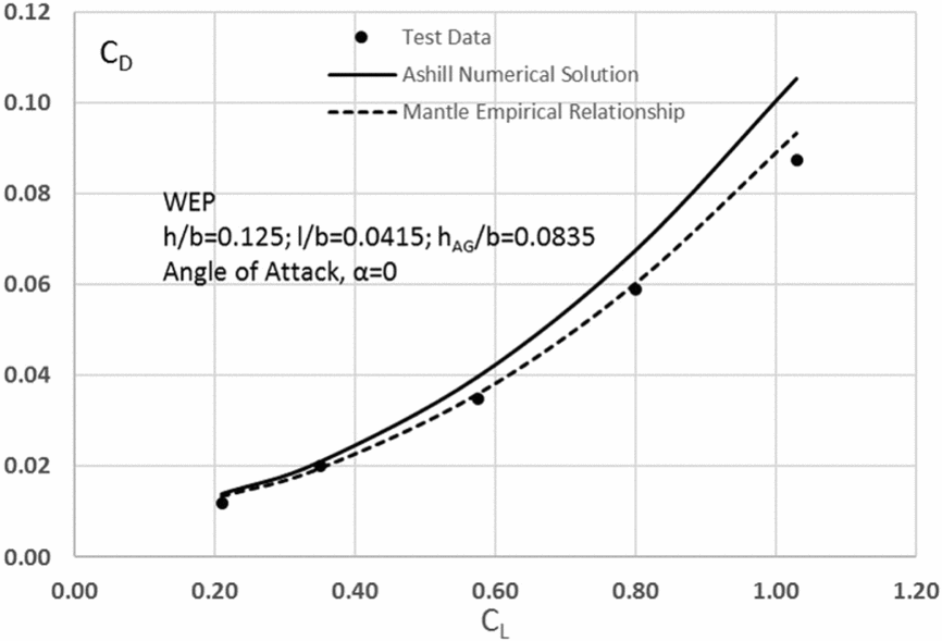
Figure 11. Drag polar at h/b = 0.125 (WEP) (A = 2).

Figure 12. Drag polar at h/b = 0.0835 (WEP) (A = 2).
Included in Figs 11 and 12 are the empirical results using the earlier developed relationship Equation (24) that related geometry of h/b and hAG/b to the induced drag factor (1 – σ). This relationship provides a reasonable prediction for a wide range of lift coefficients (0 < CL < 0.80) pending more complete understanding of the experimental results and influence of vortex formation. The α = 0 case has been used in the construction of Ashill's curves in Fig. 6.
With charts such as Fig. 8, it now becomes possible to make preliminary design decisions about the wing configuration (with and without end plates). Consider three possible designs called WIG(A), WIG(B) and WIG(C). These are displayed in Fig. 13.

Figure 13. Three possible WIG designs with and without end plates.
Assume WIG(A) has been designed to operate at a low height above the surface (h/b = 0.04) and has no end plates. This means the air gap is the same with a value of (hAG/b = 0.04). Figure 13 shows that such a design would have a value of induced drag of 28% of the value when flying out of ground effect. If the craft is expected to operate over waves, such a small air gap would raise questions of safety and the design height might be raised to (h/b = 0.10), and the new WIG(B) design would now have a higher induced drag value of 50% of the out of ground effect value. If a third design (WIG(C)) is introduced with end plates with a depth of (l/b = 0.10) and is operated with the same air gap (hAG/b = 0.04), it is seen that the induced drag has been lowered to give a new value at approximately 36% of the OGE value.
WIG(C) is an improvement at 36% OGE induced drag over WIG(B) with its higher value of 50% OGE induced drag, and at the same time gives a wave clearance improvement (h/b = 0.14) over WIG(A) with its h/b = 0.04. Such charts allow for rapid design choice options ready for more detailed design optimisation with other aerodynamic and structural characteristic considerations.
7.0 LIFT-DRAG RATIO OF WINGS WITHOUT END PLATES
Using the earlier developed relationships, it becomes possible to express the lift-drag ratio (L/D) for wings operating in ground effect as:
 $$\begin{equation}
\frac{L}{D} = \frac{{{C_{Lo}} + {\raise0.7ex\hbox{${\partial {C_L}}$} \!
/ \!\lower0.7ex\hbox{${\partial \alpha }$}}\alpha }}{{{C_{Do}} + {K_2}\left( {1 - \sigma } \right)\frac{{C_L^2}}{{\pi A}}}}
\end{equation}$$
$$\begin{equation}
\frac{L}{D} = \frac{{{C_{Lo}} + {\raise0.7ex\hbox{${\partial {C_L}}$} \!
/ \!\lower0.7ex\hbox{${\partial \alpha }$}}\alpha }}{{{C_{Do}} + {K_2}\left( {1 - \sigma } \right)\frac{{C_L^2}}{{\pi A}}}}
\end{equation}$$
In this expression for the L/D, the author has added the constant modifier, K 2, to the induced drag for better agreement with experimental data. The values CLo and CDo refer to the basic lift and drag characteristics of the aerofoil at zero angle-of-attack. The maximum value of the L/D can then be shown to be:
 $$\begin{equation}
{\left( {\frac{L}{D}} \right)_{\max }} = \sqrt {\frac{{\pi A}}{{4{C_{Do}}{K_2}\left( {1 - \sigma } \right)}}}
\end{equation}$$
$$\begin{equation}
{\left( {\frac{L}{D}} \right)_{\max }} = \sqrt {\frac{{\pi A}}{{4{C_{Do}}{K_2}\left( {1 - \sigma } \right)}}}
\end{equation}$$
It was found that assuming K 2 = 0.8 gave good agreement with the available data from the experiments by Fink and Lastinger. Figures 14, 15 and 16 show the comparison between theory and test for three aspect ratios (A = 1, 2 and 4). The case for OGE flight has also been included.
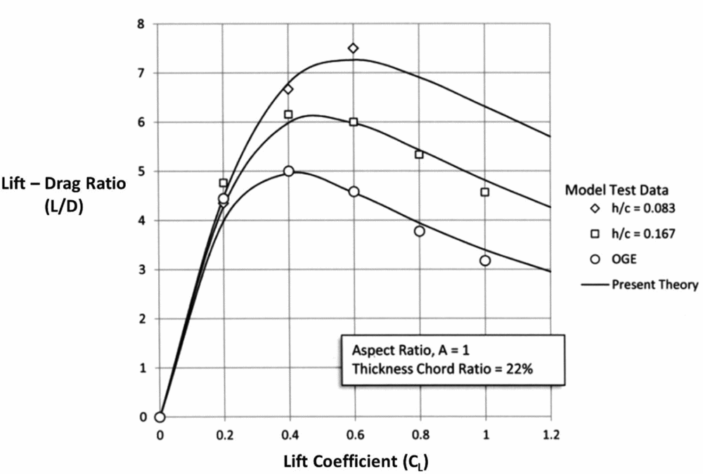
Figure 14. L/D for A = 1.

Figure 15. L/D for A = 2.
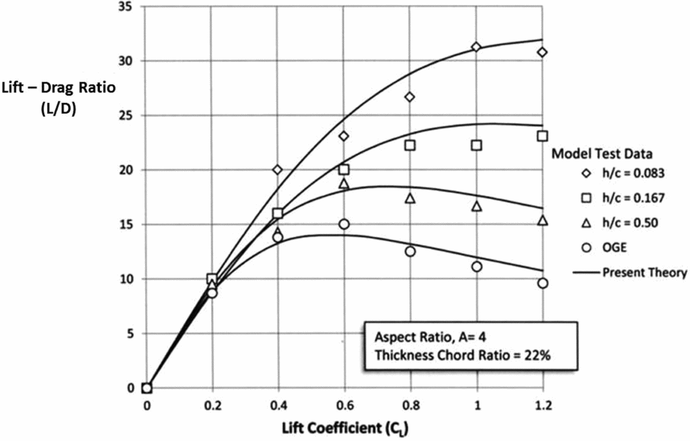
Figure 16. L/D for A = 4.
It is seen that the theory gives good agreement over a broad range of wing aspect ratios most likely to be used in such craft. It is seen that over this range of aspect ratios, the maximum value of L/D doubles approximately for each doubling of the aspect ratio and that the maximum value occurs at ever higher values of lift coefficient.
8.0 LIFT-DRAG RATIO OF WINGS WITH END PLATES
There has been only limited treatment of wings in ground effect with end plates. The original experimental work by Carter (NACA, 1961) and by Ashill (theory and test) at Cranfield (1970) provides a good starting point. While all researchers used different model geometries, operating conditions and other differences that make direct comparison difficult, enough data is available to provide general information on the aerodynamic characteristics of vortex formation in ground effect and its effect on induced drag (Di ) and the L/D of the various configurations. Carter worked with aspect ratio A = 1 thin wings (t/c = 11%). A selection of some of his results are shown in Fig. 17 for the drag polar. In the Carter models, the end plates were all flush with the wing TE (see Fig. 4) and the heights above the surface (water in his experiments) at the wing TE h′/b, which can be transformed to the height at the quarter chord point by:
 $$\begin{equation}
\frac{h}{b} = \frac{{h'}}{b} + {\raise0.5ex\hbox{$\scriptstyle 3$} \kern-0.1em/\kern-0.15em \lower0.25ex\hbox{$\scriptstyle 4$}}\frac{{\sin \alpha }}{A}
\end{equation}$$
$$\begin{equation}
\frac{h}{b} = \frac{{h'}}{b} + {\raise0.5ex\hbox{$\scriptstyle 3$} \kern-0.1em/\kern-0.15em \lower0.25ex\hbox{$\scriptstyle 4$}}\frac{{\sin \alpha }}{A}
\end{equation}$$
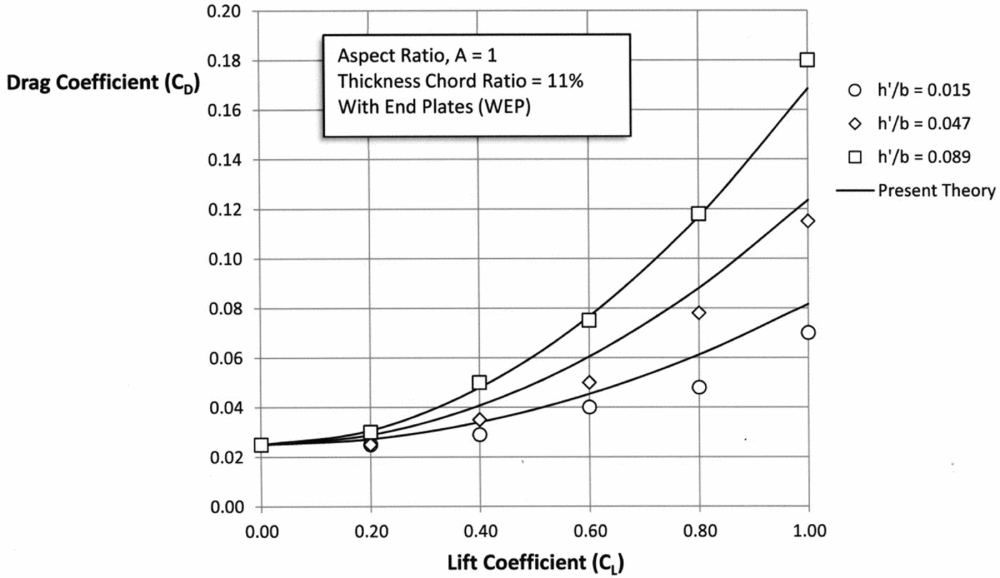
Figure 17. Drag polar for wings with end plates (Carter, 1961).
In the notation of this paper,
 $\frac{{h'}}{b} = \frac{{{h_{TE}}}}{b}$
, and the test results have been compared with the empirical equation developed earlier (see Equation (24)) using the derived induced drag factor:
$\frac{{h'}}{b} = \frac{{{h_{TE}}}}{b}$
, and the test results have been compared with the empirical equation developed earlier (see Equation (24)) using the derived induced drag factor:
 $$\begin{equation}
{\left( {1 - \sigma } \right)_{{\rm{WEP}}}} = 1.5\left( {\frac{{{h_{AG}}}}{b}} \right) + 5\left( {\frac{h}{b}} \right) - \frac{{10}}{{{{\left( {{\raise0.7ex\hbox{${{h_{AG}}}$} \!
/ \!\lower0.7ex\hbox{$b$}}} \right)}^{{\raise0.5ex\hbox{$\scriptstyle 1$} \kern-0.1em/\kern-0.15em \lower0.25ex\hbox{$\scriptstyle 5$}}}}}}{\left( {\frac{h}{b}} \right)^2}
\end{equation}$$
$$\begin{equation}
{\left( {1 - \sigma } \right)_{{\rm{WEP}}}} = 1.5\left( {\frac{{{h_{AG}}}}{b}} \right) + 5\left( {\frac{h}{b}} \right) - \frac{{10}}{{{{\left( {{\raise0.7ex\hbox{${{h_{AG}}}$} \!
/ \!\lower0.7ex\hbox{$b$}}} \right)}^{{\raise0.5ex\hbox{$\scriptstyle 1$} \kern-0.1em/\kern-0.15em \lower0.25ex\hbox{$\scriptstyle 5$}}}}}}{\left( {\frac{h}{b}} \right)^2}
\end{equation}$$
Because the endplates in these tests were flush with the wing TE, then
 $\frac{{{h_{TE}}}}{b} = \frac{{{h_{AG}}}}{b}$
. It is recognised that the relationship given in Equations (24) and (28) was derived from the results of Ashill's analysis where the end plates are not flush with the TE (see Fig. 5), but pending more rigorous theory and test treatments it is useful to see the comparison. It is seen that the expected functional form (CD
~ CL
2) is followed to an encouraging degree. The numerical values of drag at the low ground clearance heights (hTE/b = 0.089) agree well with Equation (28), with slightly less agreement as the heights are lowered to very small values (hTE/b = 0.015). This is in agreement with Prandtl's warning that at very low heights, the inviscid theories would be compromised by the boundary layer and vortex action effects.
$\frac{{{h_{TE}}}}{b} = \frac{{{h_{AG}}}}{b}$
. It is recognised that the relationship given in Equations (24) and (28) was derived from the results of Ashill's analysis where the end plates are not flush with the TE (see Fig. 5), but pending more rigorous theory and test treatments it is useful to see the comparison. It is seen that the expected functional form (CD
~ CL
2) is followed to an encouraging degree. The numerical values of drag at the low ground clearance heights (hTE/b = 0.089) agree well with Equation (28), with slightly less agreement as the heights are lowered to very small values (hTE/b = 0.015). This is in agreement with Prandtl's warning that at very low heights, the inviscid theories would be compromised by the boundary layer and vortex action effects.
A more dramatic effect can be seen in the same results for the L/D of the same tests as shown in Fig. 18. Carter observed that as the ground clearance approached very low values that the vortex action around the wings changed where the vortices weakened and contributed to an even lower value of induced drag and thus a higher value of L/D. This effect can be seen in Fig. 18.
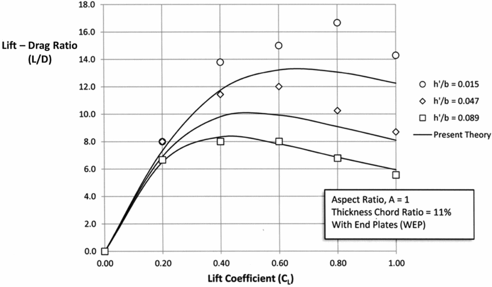
Figure 18. Lift-drag ratio for wings with end plates (Carter, 1961).
In 1970, Ashill also conducted experiments of wings with end plates to augment his theoretical treatment, albeit with different geometries of end plates that were not flush with the wing trailing edge. Two sets of results from the Ashill tests are shown in Figs 19 and 20 and compared with Prandtl's formulation for wings without end plates (see Equation (7)) and for wings with end plates using the same empirical equation derived from Equation (28).

Figure 19. Lift-drag ratio with NEP (Ashill, 1970).

Figure 20. Lift-drag ratio WEP (Ashill, 1970).
A comparison with the Carter results shows similar agreement, although a direct agreement is not possible because of the major impact of span (b) with the Carter tests conducted for A = 1 wings and the Ashill tests were conducted for A = 2 wings. The impact of span or aspect ratio is quite marked as seen in Figs 14, 15 and 16.
9.0 OBSERVED TRAILING-EDGE VORTEX FORMATIONS
In much of the available literature on wings in ground effect (both with and without end plates), frequent reference is made to the changes in the flow mechanism as wing heights become smaller, end plate depths vary and other variations are invoked. Fink and Lastinger discuss how the overall lift and drag vary through other than the induced drag changes due to such effects of ram air, profile drag of the end plates and flow around the wing at small air gaps. Carter refers to the effect of ram air, angle-of-attack effects and changes in profile drag. Ashill also notes (in his tuft grid surveys) that a similar change in flow occurred at low values of ground clearance where the vortex strength weakened as the air gap (hAG/b) became very small. In the Ashill tests, this also appeared to change the functional form of induced drag not following the expected relationship (CDi ~ CL 2) as seen in Figs 11 and 12. This departure from the expected relationship manifests itself in the L/D for the low air gap (hAG/b = 0.042) as seen in Fig. 20. Most of these assessments must be recognised as conjecture at this time pending more rigorous testing and analysis of a consistent set of wing geometries and operating conditions. Other observers(12) refer to the change on the location of the TE vortex formation shifting from the wing-tip edge (junction of the wing with the end plate) to the lower edge of the end plate as the wing end plate geometry is changed. Figure 21 shows a possible change in vortex formation.
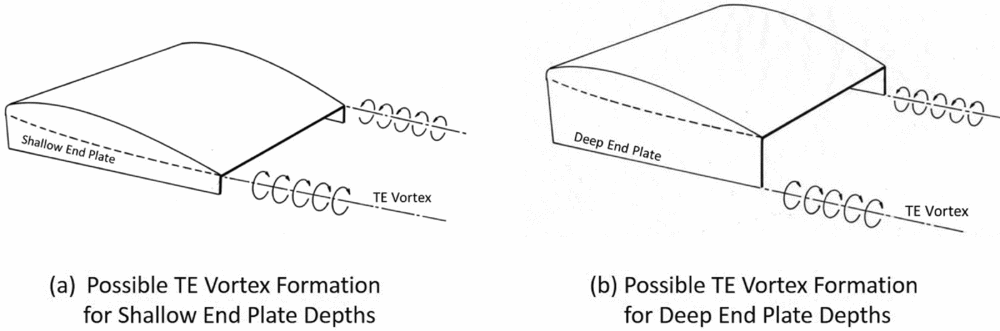
Figure 21. Possible trailing-edge vortex formations.
Some Russian designs(Reference Mantle1) have included a high-powered air jet directed aft from the lower edge of the end plates to weaken or destroy the trailing vortices of the type shown in Fig. 21(b).
While each of the researchers refer to these observations in their work, there has been no systematic treatment to study these effects, although as the Ashill experiments show (see Fig. 20 and other charts in this paper), the changes in induced drag and thus the L/D depart from the expected variation with the lift coefficient, especially at high values of lift coefficient. The data and theoretical predictions are presented here for completeness.
10.0 INDIRECT CONFIRMATION OF INDUCED DRAG RESULTS FROM OPERATIONAL CRAFT
Very little data is available from any operational craft to confirm the above theoretical results other than the model tests already cited and discussed above. It is possible, however, to obtain an indirect confirmation through use of the available information from the Russian ekranoplan craft that operated briefly from 1966–1987Footnote 1 . Three such craft are the Caspian Sea Monster (prototype in 1966), the Orlyonok used for amphibious warfare in 1972, and the Lun designed as a missile attack craft in 1987. Figure 22 shows the three craft operating over the Caspian Sea in surface effect.

Figure 22. Three Russian ekranoplans operating in surface effect.
The Russian designers used a rule of thumb in designing their craft with respect to the air gap or operating height(12). It is given as:
 $$\begin{equation}
\frac{{h_{TE}^{}}}{c} = \frac{{{H_{{\raise0.5ex\hbox{$\scriptstyle 1$} \kern-0.1em/\kern-0.15em \lower0.25ex\hbox{$\scriptstyle {30}$}}}}}}{{2c}} + 0.10
\end{equation}$$
$$\begin{equation}
\frac{{h_{TE}^{}}}{c} = \frac{{{H_{{\raise0.5ex\hbox{$\scriptstyle 1$} \kern-0.1em/\kern-0.15em \lower0.25ex\hbox{$\scriptstyle {30}$}}}}}}{{2c}} + 0.10
\end{equation}$$
This design rule for the operating height uses one half of the 30th highest wave
 $( {{H_{{\raise0.5ex\hbox{$\scriptstyle 1$} \kern-0.1em/\kern-0.15em \lower0.25ex\hbox{$\scriptstyle {30}$}}}}} )$
to characterise the sea state plus a safety margin equal to 0.10 of the wing chord. The details for each of the craft shown in Fig. 22 are provided by Mantle, but by way of illustration, the pertinent values for the Lun craft (with wing aspect ratio A = 3.53) are:
$( {{H_{{\raise0.5ex\hbox{$\scriptstyle 1$} \kern-0.1em/\kern-0.15em \lower0.25ex\hbox{$\scriptstyle {30}$}}}}} )$
to characterise the sea state plus a safety margin equal to 0.10 of the wing chord. The details for each of the craft shown in Fig. 22 are provided by Mantle, but by way of illustration, the pertinent values for the Lun craft (with wing aspect ratio A = 3.53) are:
 $$\begin{equation}
\frac{{{h_{TE}}}}{b} = 0.063\quad \frac{h}{b} = 0.12\quad \frac{l}{b} = 0.057\quad \frac{{{h_{AG}}}}{b} = 0.063
\end{equation}$$
$$\begin{equation}
\frac{{{h_{TE}}}}{b} = 0.063\quad \frac{h}{b} = 0.12\quad \frac{l}{b} = 0.057\quad \frac{{{h_{AG}}}}{b} = 0.063
\end{equation}$$
Similar analyses of the flight characteristics from photographs and videos of the three craft provide the necessary geometric values of the other two craft, which are displayed in Fig. 23.
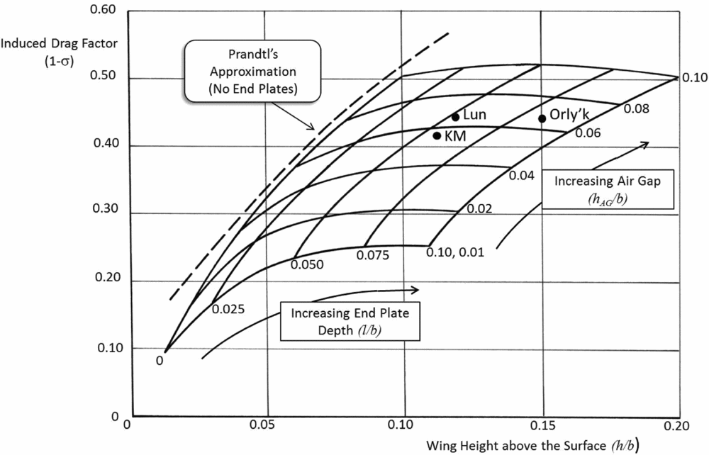
Figure 23. Projected values of reduced induced drag of ekranoplans.
From this analysis of the available in-flight photographs, it is surmised that the designers of the ekranoplan for WIG (with end plates) operating in ground effect were obtaining a reduction in induced drag of approximately 40-50% of the value experienced out of ground effect. It remains for more detailed analyses in a controlled experiment to verify these values.
11.0 SUMMARY
This paper has developed a set of closed-form solutions for the lift and induced drag characteristics of wings with and without end plates operating in ground effect. The theories and empirical relationships developed show good agreement with the experimental data collected from a variety of independent sources.
Table 1 provides a summary of the key equations.
Table 1 Summary of key equations


