2.0 SENSORS INSTALLATION

Once identified the need for real-time monitoring of HT local angle-of-attack, several options of different sensors were considered⁽Reference Eppel, Riddle and Steves¹⁾. Most of the available sensors, such as angle-of-attack vanes, smart probes, etc. would have similar calibration challenges but would significantly affect the HT structural characteristics; in addition, most of the already available sensors, due to their size and ideal locations were considered to interfere with the local airflow, thus interfering with the local ${\alpha}_{\rm{HT}}$ measurement itself.

The search for a local angle-of-attack measurement that would not significantly affect the HT structural design and be non-airflow-interferant led to a differential static pressure solution. This solution only requires small pressure ports (small holes) adequately located to be sensible to small pressure differences between the upper and lower surfaces of the HT aerofoil. Those differential pressure measures are physically correlated to local angle-of-attack variations.

The static pressure ports were designed to be located on the leading edge of the HT. This location was chosen due to two different aspects:

1. 1. It presents a higher sensitivity of static pressure coefficient $({\rm C}_{\rm{P}})$ due to $\alpha_{\rm{HT}}$ variation.

2. 2. Ease of installation and maintenance, once the pressure transducers can be installed with the removal of the HT leading edge, which is usually removable in most aircraft for several other reasons (for example, anti-ice piccolo tubes installation).

As the differential pressure ports are susceptible to blockage and local disturbances and considering the safety effects of a wrong measure for real-time monitoring during the flight test, a conservative, robust and redundant design was chosen: the differential pressure ports were distributed along ten chord positions for two distinct sections along the HT span. For this purpose, an averaging and a voting algorithm were employed for the final ${\alpha}_{\rm{HT}}$ measurement.

Figure 1 shows the schematic architecture of the system.

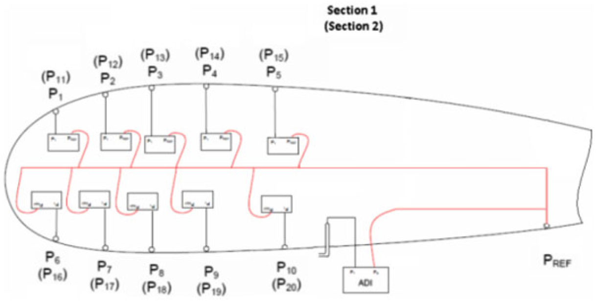
Figure 1. Schematic system architecture of the system

Considering the needs for a quick time response, good accuracy and resolution, the Honeywell PPT0002DNN2VB-S068 differential pressure sensor was chosen.

• Honeywell PPT0002DNN2VB-S068 specifications⁽²⁾:

• Digital Accuracy: $\pm0.05\%$ FS

• Analog Accuracy: $\pm0.06\%$ FS

• Operating Temperature: $-40\ {\rm to}\ 85^{\circ}{\rm C}$

• Storage Temperature: $-55\ {\rm to}\ 90^{\circ}{\rm C}$

• Sample Rate: 8.33ms to 51.2min

• Digital Resolution: up to $\pm0.0011\%$ FS

• Analog Resolution: 1.22mV

• Long Term Stability: 0.025% FS per year

• Range: $\pm2\ {\rm psi}$

Since the PPT0002DNN2VB-S068 needs to be connected to the reference pressure using capillary tubes, to avoid a possible pressure wave lag in the final measure, a single static pressure $({\rm P}_{\rm{ref}})$ reference port was chosen and positioned as close as possible to transducers minimising the tubes length and consequently its internal air volume. The ${\rm P}_{\rm{ref}}$ was in the lower side of HT.

All 20 differential pressure transducers are connected to a reference static pressure port $({\rm P}_{\rm{ref}})$ . Consequently, each transducer measures a differential pressure $\Delta {\rm P}_{\rm n}$ relative to the reference static port ${\rm P}_{\rm{ref}}$ .

It is possible to convert the measure from the reference point to free-stream values by Equation (1), which uses free-stream static pressure $({\rm P}_{\infty})$ and dynamic pressure $({\rm Q}_{\infty})$ . These quantities may be provided by the aircraft’s anemometric system or measured by dedicated flight-test instrumentation sensors, such as a trailing cone and aircraft Kiel pitot.

(1) \begin{equation} C_{P_{n} } =\frac{\Delta P_{n} +P_{ref} -P_{\infty } }{Q_{\infty}} \label{eqn1} \end{equation}

The local dynamic pressure was measured through a Kiel pitot installed on the lower side of the HT using a pre-existent access panel for the ease of installation and maintenance. The Kiel pitot vertical position was chosen to keep it out of the boundary layer.

Figure 2 provides detailed information for the position of installed pressure ports, pressure transducers and Kiel pitot.

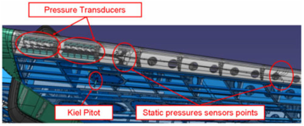
Figure 2. HT sensors positions and installation.

3.0 PRE-FLIGHT SENSORS CALIBRATION

The adopted differential pressure solution does not provide a direct local angle-of-attack measurement, thus, requiring the means to convert differential pressure measurements in angle-of-attack.

To develop the proper correlation between differential pressure and local angle-of-attack, an estimation of the $\alpha_{\rm{HT}}$ (pre-flight) was done using CFD.

In order to derive the relations, CFD simulations were performed with Metacomp Technologies CFD++ code⁽³⁾ to simulate subsonic airflow conditions.

Three different types of CFD simulations were run:

• Complete aircraft (WBPNH) with HT incidence variation;

• Wing-Body-Pylon-Nacelle tailless aircraft (WBPN);

• Body-Horizontal-Tail (BH) wingless aircraft with different elevator deflections.

The grids are generated using the gridding guidelines based on the EMBRAER experience⁽Reference Scalabrin, Ciloni, Antunes, Becker, Souza and Granzoto⁴⁾. The flow is modelled using the Reynolds-averaged Navier-Stokes equations (RANS) with turbulence model closures. The time march is performed using a point-implicit method and multigrid method for convergence acceleration. In this work, the SA turbulence model is employed⁽Reference Sparlat⁵⁾ and is a well-established closing model for aerospace industrial applications.

Local ${\alpha}_{\rm{HT}}$ for each section takes into consideration the three effects ${\alpha}_{\rm{HT1}}$ , ${\alpha}_{\rm{HT2}}$ and ${\alpha}_{\rm{HT3}})$ according to Equation (2).

(2) \begin{equation} \alpha _{HT_{S} } =\alpha _{HT1_{S} } +\alpha _{HT2_{S} } +\alpha _{HT3_{S} } \label{eqn2} \end{equation}

Where:

S denotes the HT section (1 or 2) and the terms are:

TERM $\alpha_{HT1}$

The ${\alpha}_{\rm{HT1}}$ is the direct correlation between differential pressure measurements and local angle-of-attack. This correlation for each section S is a function of ${\rm C}_{\rm P}$ and elevator deflection. The final ${\alpha}_{\rm{HT1}}$ is the mean of the values calculated for each of the ten sensors, Equation (3). Figure 3 shows Body and Horizontal Tail mesh with two different elevator deflections.

Figure 3. Body-Horizontal-Tail mesh – with elevator two different elevator deflections.

(3) \begin{equation} \alpha _{HT1_{S} } =f(C_{Pn} ,\delta _{e} )=\frac{1}{10} \times \sum _{n=1}^{10}\alpha _{HT1n} \label{eqn3} \end{equation}

The Body-Horizontal-Tail (BH) CFD results were post-processed to provide $\alpha_{\rm{HT1}}$ , i.e. the direct correlation between differential pressure and local angle-of-attack, for different elevator angles. For each pressure port location, a local angle-of-attack $\alpha_{\rm{HT1}}$ was derived as a function of ${\rm C}_{\rm P}$ and elevator deflection. As these runs have no wing effect, the HT angle-of-attack is the same as free-stream angle-of-attack. Figure 4 shows the correlation between ${\rm C}_{\rm P}$ and ${\alpha}_{\rm{HT1}}$ for the five pressure ports at upper side of HT in the section 1 with zero elevator deflection.

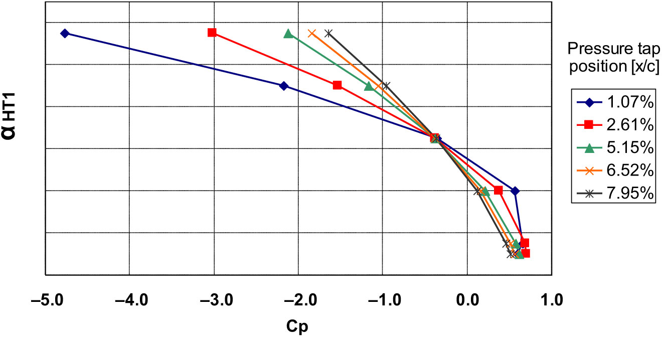
Figure 4. : Example of $\alpha_{\rm{HT1}}$ as function of ${\rm C}_{\rm P}$ for some pressure taps.

TERM $\alpha_{HT2}$

The $\alpha_{\rm{HT2}}$ is a function of aircraft free-stream angle-of-attack $(\alpha)$ and flap deflection angle $(\delta_{flap})$ , since the wing lift and downwash interferes with local HT airflow and changes the chordwise and spanwise distribution of local lift on HT.

(4) \begin{equation} \alpha _{HT2_{S} } =f(\alpha ,\delta _{flap} ) \label{eqn4} \end{equation}

The $\alpha_{\rm{HT2}}$ was calculated using WBPN CFD runs (without HT) with wing interference results calculated at 25% of local HT chord virtual position for each spanwise HT section, as it may be seen by Fig. 5. Figure 6 shows the local $\alpha$ spanwise distribution as a function of free-stream a for the landing flaps configuration.

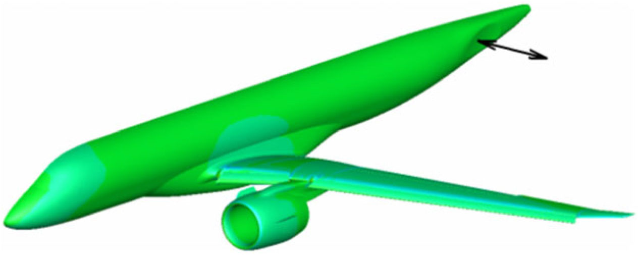
Figure 5. Wing-Body-Pylon-Nacelle configuration CFD runs showing wing and engine effects on local virtual HT position.

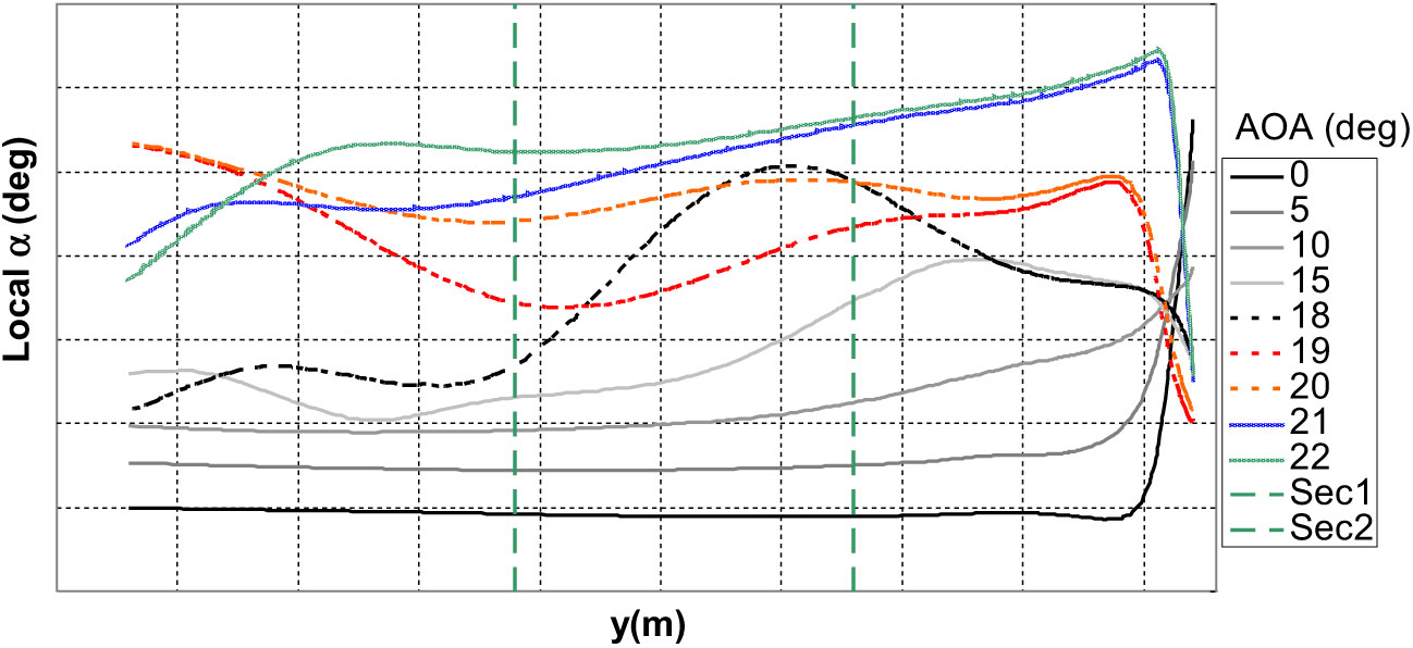
Figure 6. Local angle-of-attack at virtual HT position as a function of span position for various aircraft angle-of-attack – Landing flaps configuration.

TERM $\alpha_{HT3}$

$\alpha_{HT3}$ is a function of HT incidence $({\alpha}_{\rm{HT3}})$ , since the relative geometric position of the HT changes the aerodynamic interference characteristics between wing-tail and fuselage-tail, thus changing local HT pressure distribution. The ${\alpha}_{\rm{HT3}}$ for each section is an interference correction, which is a function of free-stream angle-of-attack, flap deflection angle and HT incidence.

(5) \begin{equation} \alpha _{HT3_{S} } =f(\alpha ,\delta _{flap} ,I_{HT} ) \label{eqn5} \end{equation}

The $\alpha_{\rm{HT3}}$ was calculated through CFD runs with WBPNH configuration with $I_{HT}$ incidences of $0^\circ, -3^\circ$ and $-6^\circ$ , thus providing corrections for the interference due to the local geometric incidence.

The final value of ${\alpha}_{\rm{HT}}$ is the mean of the calculated values for each of the two spanwise sections.

(6) \begin{equation} \alpha _{HT} =\frac{1}{2} \times \sum _{S=1}^{2}\alpha _{HT_{S} } \label{eqn6} \end{equation}

Figure 7 compares ${\alpha}_{\rm{HT}}$ components contribution during a stall manoeuvre. The plot shows that ${\alpha}_{\rm{HT1}}$ is the most significant component when compared to ${\alpha}_{\rm{HT2}}$ and ${\alpha}_{\rm{HT3}}$ by one order of magnitude. That is because ${\alpha}_{\rm{HT2}}$ and ${\alpha}_{\rm{HT3}}$ are interference corrections factors, and ${\alpha}_{\rm{HT1}}$ is directly correlated to C ${}_{\rm P}$ .

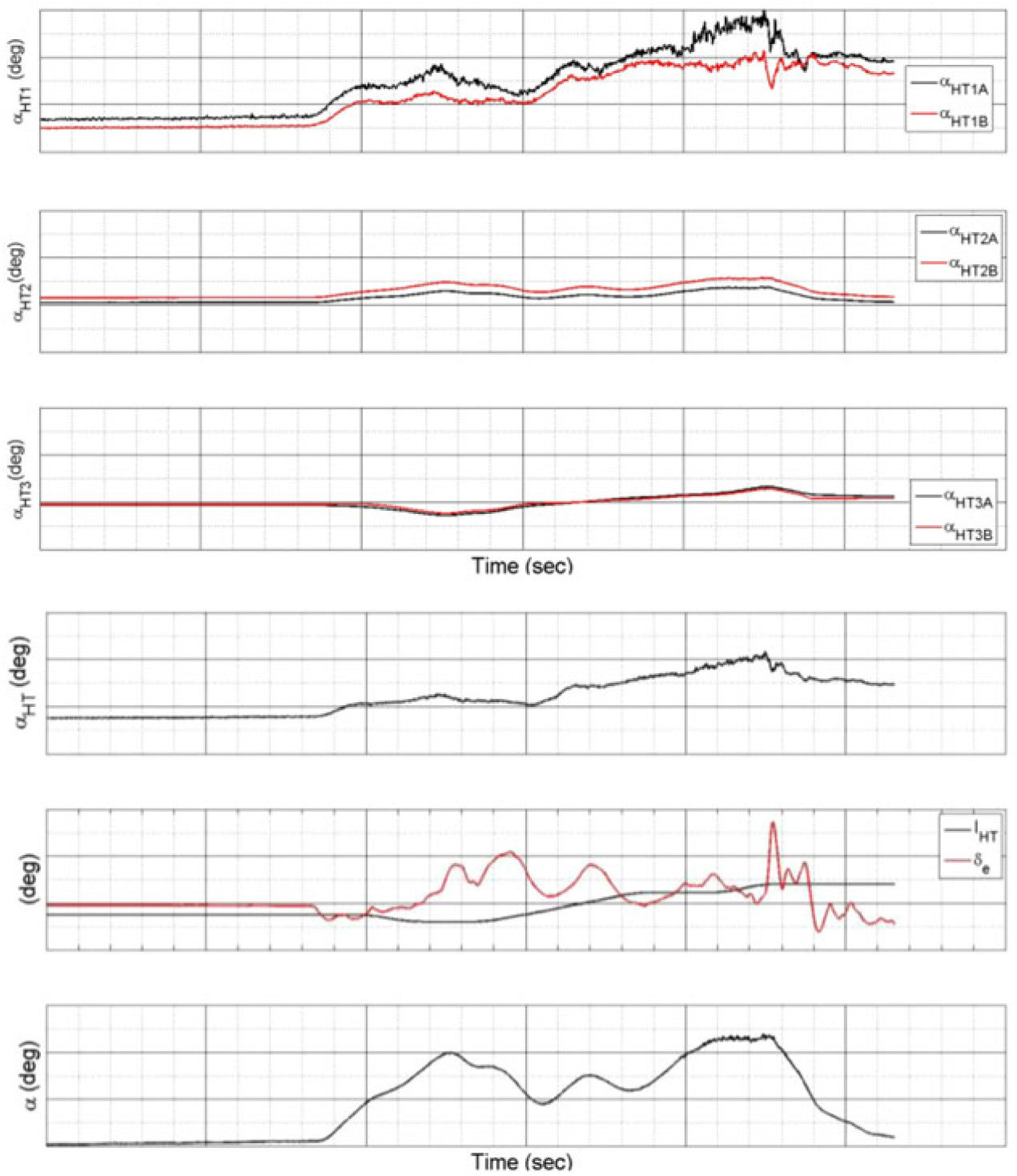
Figure 7. ${\alpha}_{\rm{HT}}$ components contribution comparison during a flight-test stall manoeuvre.

4.0 FLIGHT-TEST CALIBRATION

The flight-test calibration of ${\alpha}_{\rm{HT}}$ was based on the principle that when the aircraft angle-of-attack is kept constant, wing downwash may also be assumed constant. If it is possible to change HT incidence without changing aircraft angle-of-attack, the resultant change in HT incidence $(\Delta{\rm I}_{\rm HT})$ should be equal to the change in local angle-of-attack $(\Delta{\alpha}_{\rm{HT}})$ .

The flight-test procedure was based on the following steps:

• Trim the aircraft in a specified condition.

• Jam the elevator from the same side of sensors installation in a specified condition using a pre-defined function of flight-controls computer.

• Mistrim the aircraft using the trim switch and control the aircraft using the opposite side elevator to compensate for the mistrim. This elevator is not jammed and does not influence the pressure sensors because it is not located in the same side of the pressure sensors.

• Keep airspeed and aircraft angle-of-attack constant during manoeuvre.

For static conditions, local ${\alpha}_{\rm{HT}}$ is a function of aircraft downwash and local tail incidence. Equations (7) and (8) describe, respectively, the conditions before and after the aircraft is mistrimmed.

(7) $${{\alpha }_{HT1}}={{\alpha }_{1}}-{{\varepsilon }_{1}}+{{I}_{HT1}}$$

(8) $${{\alpha }_{HT2}}={{\alpha }_{2}}-{{\varepsilon }_{2}}+{{I}_{HT2}}$$

The flight-test calibration manoeuvre is performed varying the ${\rm I}_{\rm{HT}}$ and keeping the remaining parameters constant, thus:

(9) $${{\alpha }_{1}}={{\alpha }_{2}}$$

(10) $${{\varepsilon }_{1}}={{\varepsilon }_{2}}$$

Subtracting Equation (7) from Equation (8) results:

(11) $${{\alpha }_{HT1}}-{{\alpha }_{HT2}}={{I}_{HT1}}-{{I}_{HT2}}$$

(12) $$\Delta {{\alpha }_{HT}}=\Delta {{I}_{HT}}$$

The quantities ${\Delta \rm{I}}_{\rm{HT}}$ and ${\Delta\alpha}_{\rm{HT}}$ may be calculated in relation to trimmed initial condition. Because Equation (12) is not satisfied exactly in flight-test conditions, a calibration factor, ${\rm K}_1$ is introduced, as shown in Equation (13).

(13) $$ \begin{equation} \Delta I_{HT} =K_{1} \times \Delta \alpha _{HT} \label{eqn13} \end{equation} $$

This process is repeated for each elevator position, thus providing corrections for the direct relationship between local angle-of-attack, elevator deflection and local ${\rm C}_{\rm P}$ . This process is also repeated for different angle-of-attacks and flap deflections and, consequently, provides corrections to the interference between wing and HT.

A flight data comparison between ${\Delta \rm{I}}_{\rm{HT}}$ and ${\rm K}_{1} \times {\Delta\alpha}_{\rm{HT}}$ is presented in Figs 8, 9 and 10. The good correlation shows that the calibration factor was sufficient to capture the effects of wing interference and local pressure distribution for different elevator deflections. It is important the calibration has good physics modelling to increase the correlation between theoretical and flight-test data.

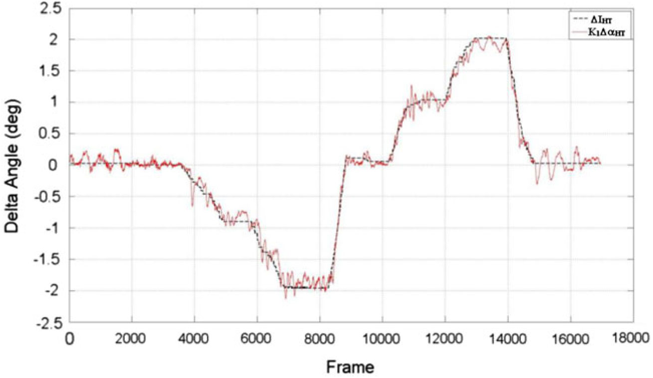
Figure 8. Calibration flight-test results – comparison between ${\Delta{\rm I}}_{\rm{HT}}$ and ${\rm K}_{1}\Delta\alpha_{\rm{HT}}$ – Cruise Flaps Configuration.

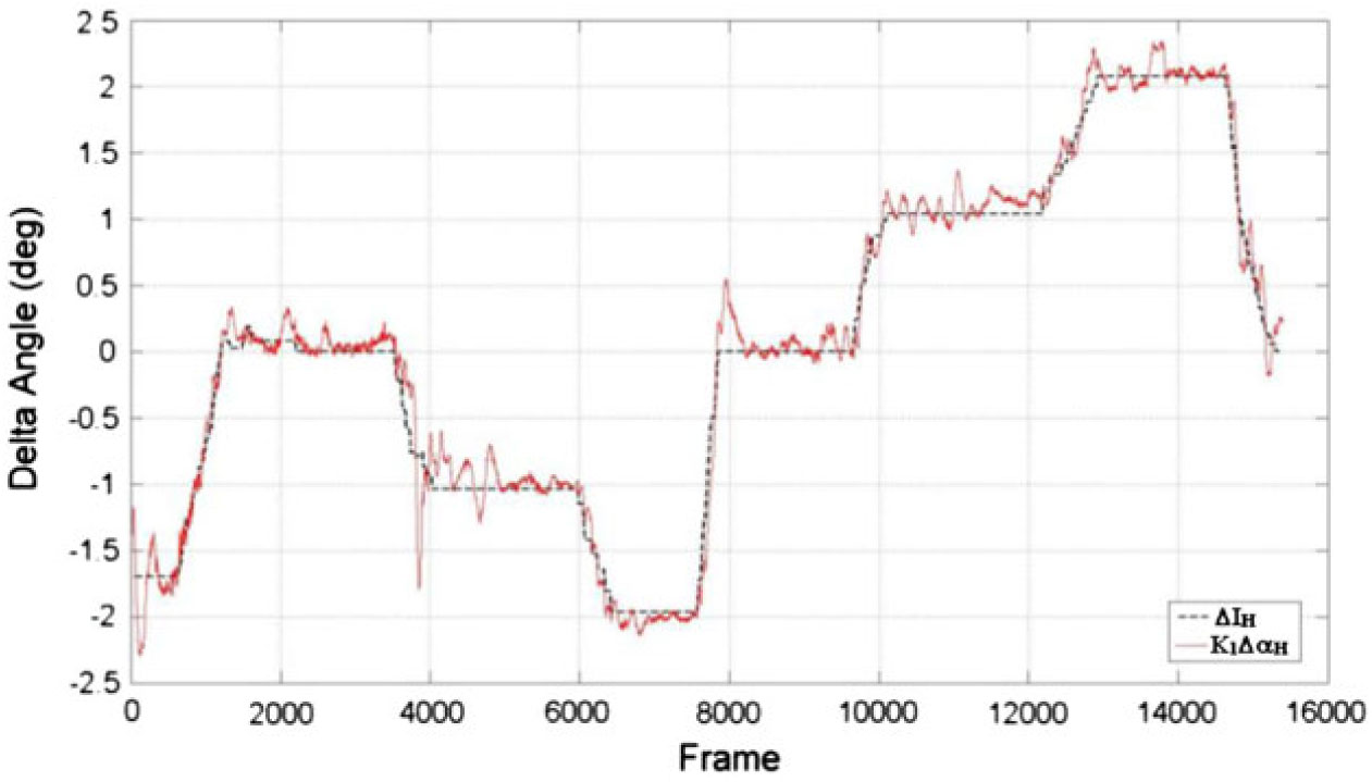
Figure 9. Calibration flight-test results – comparison between ${\Delta{\rm I}}_{\rm{HT}}$ and ${\rm K}_{1}\Delta\alpha_{\rm{HT}}$ – Take-off Flaps Configuration.

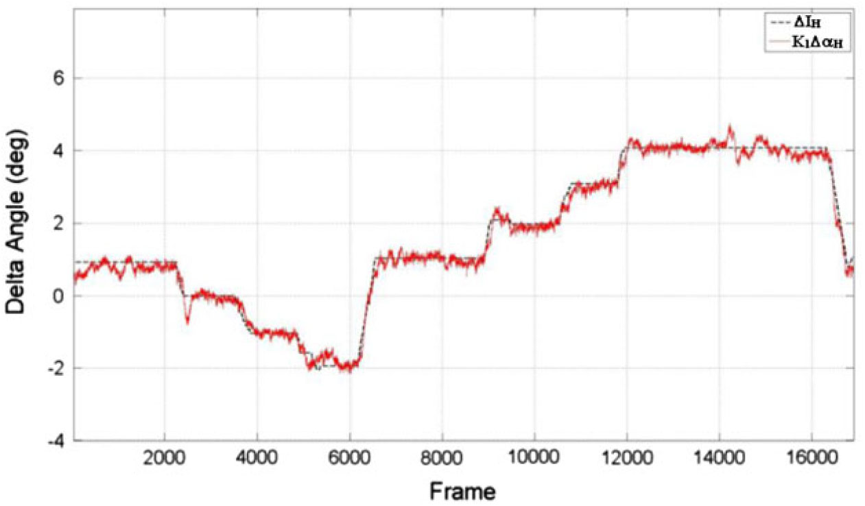
Figure 10. Calibration flight-test results – comparison Between ${\Delta{\rm I}}_{\rm{HT}}$ and ${\rm K}_{1}\Delta\alpha_{\rm{HT}}$ – Landing Flaps Configuration.

5.0 FLIGHT-TEST RESULTS

The local HT angle-of-attack and dynamic pressure and the wing downwash are physically correlated to the aircraft inherent aerodynamic stability.

In the earlier stages of aircraft development, before first flight, wind-tunnel data is used to predict ${\alpha}_{\rm{HT}}$ and $\varepsilon$ . These data are also fed into flight dynamics simulation models to evaluate the aircraft handling characteristics, function hazard analysis, design, etc. It is important to understand how the measured variables compare to predictions based on wind-tunnel data in the early stages of aircraft flight-test development for safe envelope expansion and for aircraft control laws development and validation.

The differences between flight-test and wind-tunnel data may be used to improve existent flight-mechanics models. Data may be extrapolated for the more critical conditions, such as higher angle-of-attack and aft CG stall manoeuvres. These new predicted data then may be compared with real-time measurements of $\varepsilon$ and ${\alpha}_{\rm{HT}}$ during stall manoeuvres, providing safe flight-test stop criteria if these parameters are out of a pre-determined range.

In aircraft with fly-by-wire systems, the control laws may be susceptible to aerodynamic model errors, particularly in the higher $\alpha$ region. The downwash and local-angle-of-attack measurements may also be used in conjunction with parameter-estimation techniques to improve linear models used when updating controls laws gains. The early update of flight-controls laws is important to improve flight-test efficiency and to provide safer flight-test expansion.

During the stall manoeuvres, the wing downwash $(\varepsilon)$ may be computed for each time (t) step as a function of wing angle-of-attack $(\alpha)$ , measured local angle-of-attack $({\alpha}_{\rm{HT}})$ and HT incidence $({\rm{I}}_{\rm{HT}})$ . If the manoeuvre is not quasi-static, i.e. with high pitch and $\alpha$ rates, the downwash lag $(\tau)$ and the increase in local HT $\alpha$ due to the pitch rate $({\alpha}_{\rm{HTdyn}})$ shall be considered:

(14) $$ \begin{equation} \varepsilon (t-\tau )=\alpha (t)-\alpha _{HT} (t)+\alpha _{HTdyn} (t)+I_{HT} (t) \label{eqn14} \end{equation} $$

Figure 11 shows such an example of computation that may be calculated in real-time during the execution of stall manoeuvres. It shows a time-history comparison between flight-test and wind-tunnel simulation data for the parameters angle-of-attack, downwash, local HT angle-of-attack, HT incidence and elevator deflection.

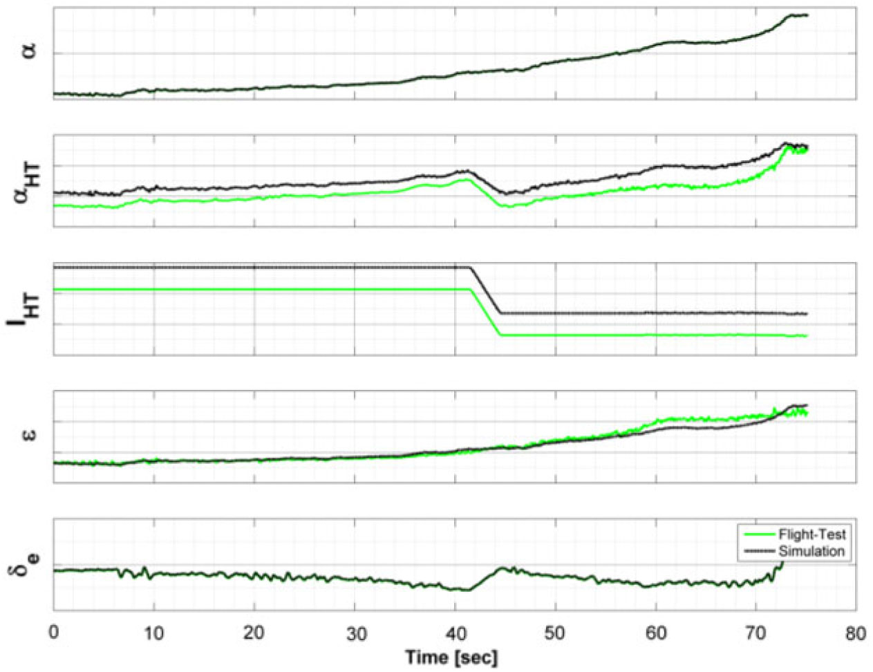
Figure 11. $\alpha_{\rm{HT}}$ and $\varepsilon$ comparison between simulation based on wind tunnel data and flight-test data during a stall manoeuvre – Cruise Flaps Configuration.

The measurement of HT characteristics was also combined with flow visualisation techniques to provide information for validation and understanding of the aerodynamic characteristics of HT airflow. Figure 12 shows the flow visualisation using tufts combined with measurements of HT angle-of-attack during a high incidence flight-test manoeuvre.

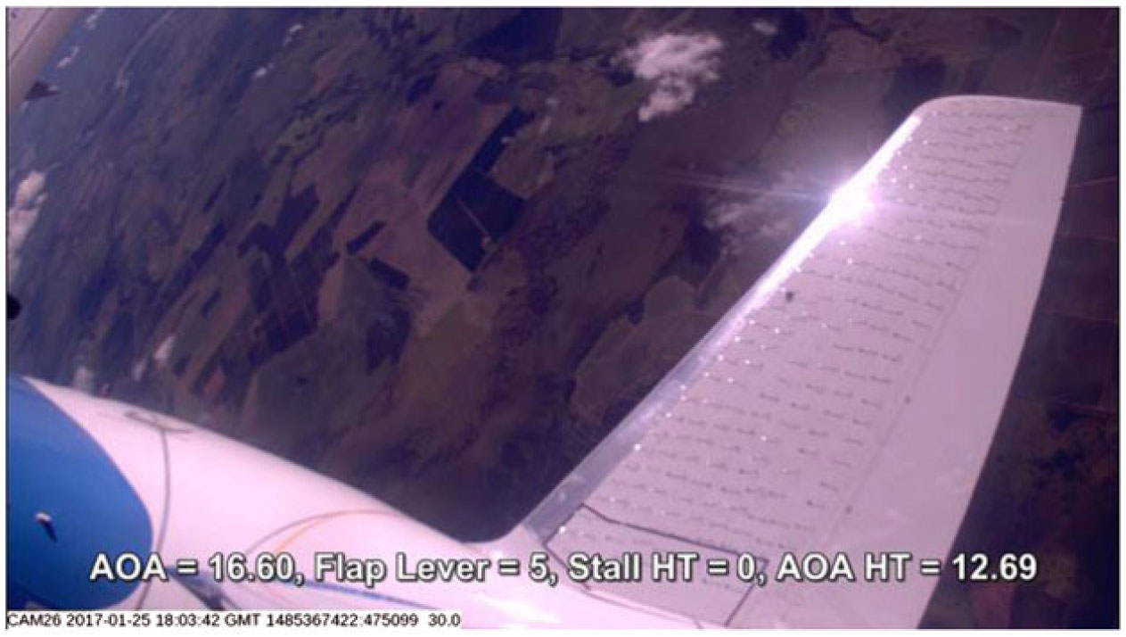
Figure 12. Tufts flow visualisation combined with HT measurements during a high incidence flight-test manoeuvre.

Crossplots of wing downwash and aircraft angle-of-attack are shown in Figs 13 to 16 for cruise, low take-off, high take-off and landing flaps configurations. The plots compare flight-test data (with and without calibration) with wind-tunnel data.

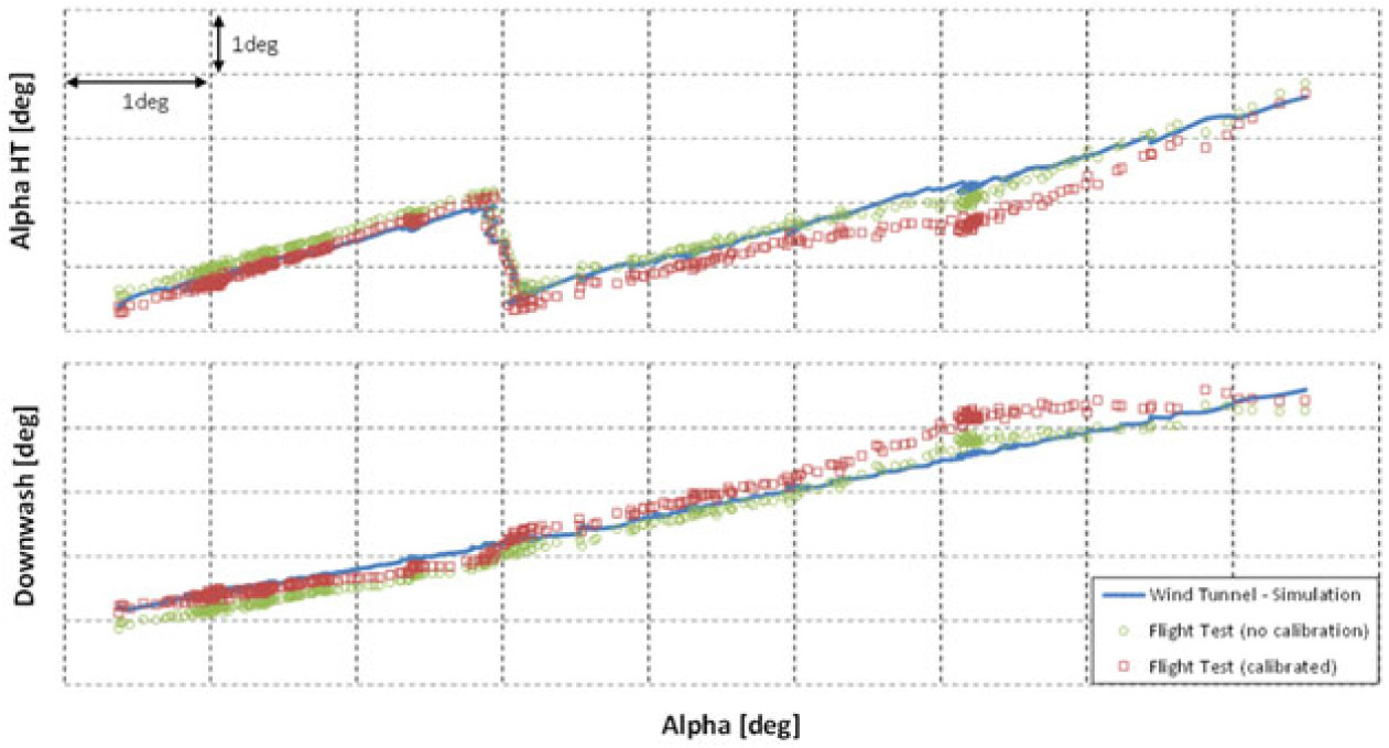
Figure 13. Local $\alpha_{\rm{HT}}$ and downwash comparison between wind-tunnel data and flight-test data during a stall manoeuvre – Cruise Flaps Configuration.

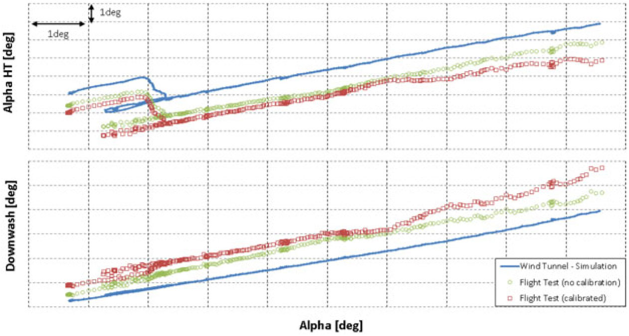
Figure 14. Local $\alpha_{\rm{HT}}$ and downwash comparison between wind-tunnel data and flight-test data during a stall manoeuvre – Low Take-off Flaps Configuration.

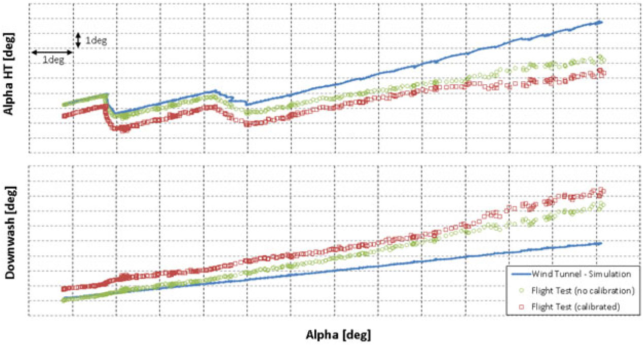
Figure 15. Local $\alpha_{\rm{HT}}$ and downwash comparison between wind-tunnel data and flight-test data during a stall manoeuvre – High Take-off Flaps Configuration.

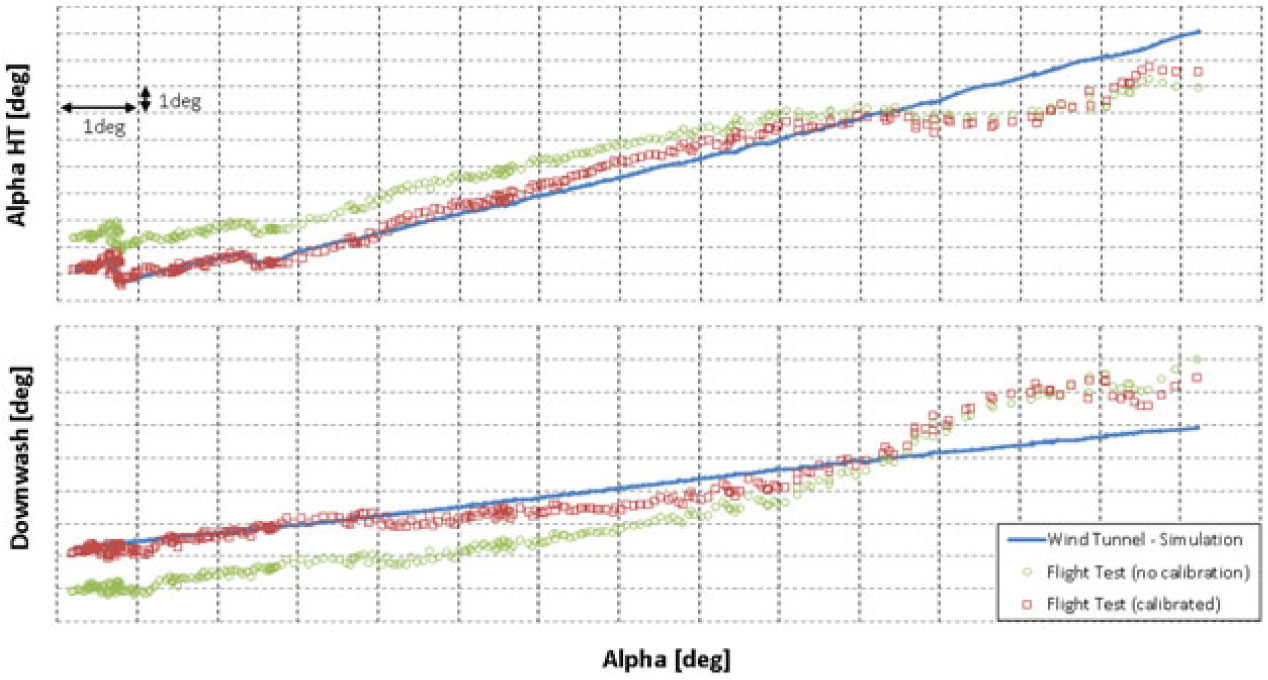
Figure 16. Local $\alpha_{\rm{HT}}$ and downwash comparison between wind-tunnel data and flight-test data during a stall manoeuvre – Landing Flaps Configuration.

The results show that the differences between flight-test and wind-tunnel data increase for higher angles-of-attack, probably due to higher interferences caused by wing and engine flow over the HT. These interferences may have different aerodynamic behaviour between wind-tunnel and flight-test (due to inherent wind-tunnel limitations such as geometric and Reynolds number differences) and may affect the measurement and calibration of $\alpha{}_{\rm HT}$ itself.

The dynamic pressure ratio as a function of aircraft angle-of-attack is shown in Figs 17 to 20 for cruise, low take-off, high take-off and landing flaps configurations.

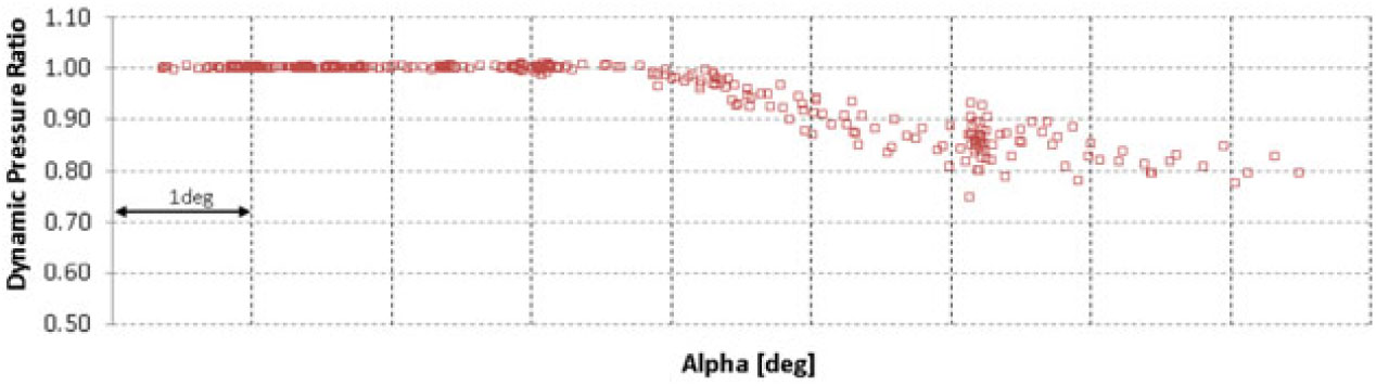
Figure 17. Flight-test measurement of dynamic pressure ratio between local and global dynamic pressure $(\eta)$ – Cruise Flaps Configuration.

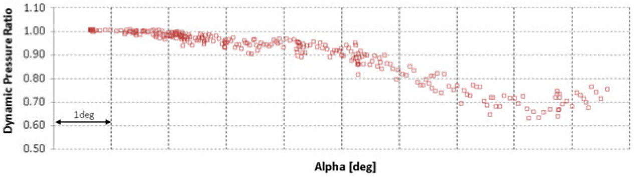
Figure 18. Flight-test measurement of dynamic pressure ratio between local and global dynamic pressure – Low Take-off Flaps Configuration.

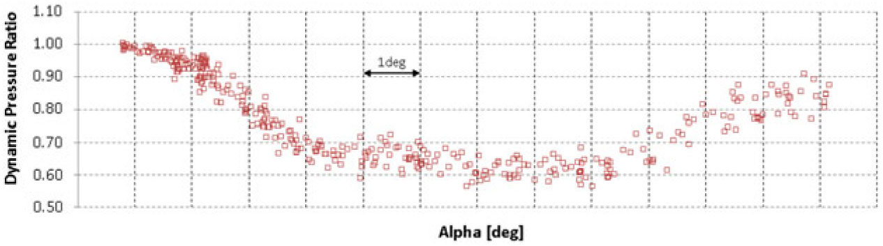
Figure 19. Flight-test measurement of dynamic pressure ratio between local and global dynamic pressure $(\eta)$ – High Take-off Flaps Configuration.

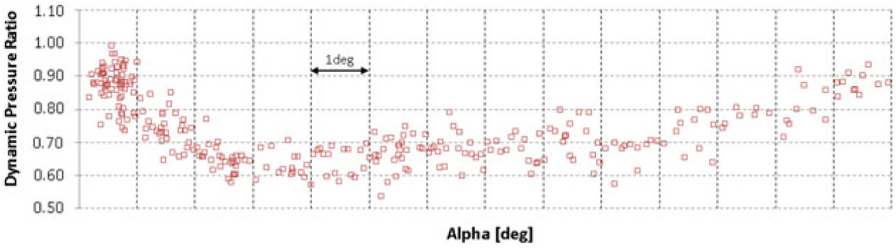
Figure 20. Flight-test measurement of dynamic pressure ratio between local and global dynamic pressure $(\eta)$ – Landing Flaps Configuration.

The results show a significant loss of dynamic pressure at medium angles-of-attack, which decreases aircraft longitudinal stability and elevator efficiency. However, in the more deflected flaps configurations, which are the critical conditions for stall characteristics, the local dynamic pressure starts to increase again near the stall angle-of-attack, improving stability and control characteristics.

If such curves of Figs 13 to 16 are linearized in the linear region of each curve, the wing downwash $({\varepsilon})$ may be written as a function of downwash for zero angle-of-attack $({{\varepsilon}_{0}})$ and a downwash slope $({{\rm d}\varepsilon/{\rm d}\alpha})$ , as in Equation (15).

(15) $$\varepsilon ={{\varepsilon }_{0}}+d\varepsilon /d\alpha $$

Table 1 compares the linearized downwash parameters between flight-test and wind-tunnel data.

Table 1 Differences between flight-test results and estimated wind-tunnel parameters $\varepsilon_{0}$ and $\text{d}\varepsilon/\text{d}\alpha$

In general, the differences between flight-test and wind-tunnel data (both in the linear and non-linear region) have shown that the expected maximum ${\alpha}_{\rm{HT}}$ that would be achieved in the most critical manoeuvres would always be less than the simulations model predicted, providing a safety margin for envelope expansion.