


Nomenclature
- CAD
-
Computer-Aided Design
- CFD
-
Computational Fluid Dynamics
- FAA
-
Federal Aviation Administration
- GAMG
-
Geometric-Algebraic Multi Grid
- ISA
-
International Standard Atmosphere
- NS
-
Navier-Stokes
- RANS
-
Reynold-Averaged Navier-Stokes
- S-A
-
Spalart-Allamaras
- SHM
-
snappyHexMesh
- STL
-
Stereolithography
- VRESIM
-
Virtual Research Simulator
- U
-
velocity magnitude and direction
- p
-
kinematic pressure
- P
-
pressure
-
 $\boldsymbol\rho $
-
air density
- M
-
mach number
- a
-
speed of sound
-
$\boldsymbol\nu $
-
kinematic viscosity
-
$\tilde{\boldsymbol\nu} $
-
turbulent kinematic viscosity
-
$\boldsymbol\mu $
-
dynamic viscosity
- T
-
temperature
-
$\boldsymbol\alpha $
-
angle-of-attack
-
${\textbf{{C}}_{\textbf{{L}}}}$
-
lift coefficient
-
${{\textbf{{C}}}_{\textbf{{D}}}}$
-
drag coefficient
-
${{\textbf{{C}}}_{{{\textbf{{m}}}_{\textbf{{y}}}}}}$
-
pitching moment coefficient


1.0 Introduction
AVIATION has improved over the decades thanks to the use of aircraft modeling techniques and methodologies [Reference Filippone, Zhang and Bojdo1–Reference Bacchini, Cestino, Van Magill and Verstraete5]. Aerodynamics is one aspect of aircraft design that must be very well modeled. Aerodynamic models can be developed from flight data [Reference Filippone, Parkes, Bojdo and Kelly6] or from aircraft design parameters (in the absence of flight test data) [Reference Liem, Mader and Martins7–Reference Segui and Botez12]. This paper focuses on the latter category. To develop an aerodynamic model from its geometrical characteristics, it is necessary to analyse the fluid behaviour around the aircraft from flow equations. Currently, the most accurate equations for modeling the fluid motion around a solid are the Navier-Stokes equations (NS). To help in NS resolutions, numerical approaches such as Computational Fluid Dynamics (CFD) have been developed [Reference Liauzun13, Reference Huvelin, Dequand, Lepage and Liauzun14].
While the most commonly used CFD commercial software packages are StarCCM+ and ANSYS Fluent [Reference Zou, Zhao and Chen15], open source and free software have also been released, and they are now available on a significant part of the market. The “editable” aspect of open-source codes is particularly appreciated by companies to develop in-house algorithms, adapted to their computer resources and to their customer research and development projects [Reference He, Mader, Martins and Maki16–Reference Secco, Kenway, He, Mader and Martins18].
Among open-source CFD software, OpenFoam software is the most widely used [19], and it is becoming more and more popular in the industry as it has gained considerable credibility in recent years (since 2016) [19]. OpenFoam has an impressive number of settings that can be tuned to set up a mesh design or a simulation case (i.e. choice of the solver, turbulence model, resolution scheme, etc.).
From the literature review, it has been observed that the OpenFoam toolbox was used for a wide range of applications, such as gas flow modeling (Mach number from 6 to 12.7) [Reference Le, Greenshields and Reese20], incompressible flows [Reference Sorribes-Palmer, Sanz Andres, Figueroa, Donisi, Franchini and Ogueta21], high lift modeling [Reference Ashton and Skaperdas22], ice accretion modeling [Reference Li and Paoli23], landing gear noise [Reference Hou, Angland and Scotto24], etc. Despite the general applications available using OpenFoam toolbox, the OpenFoam meshing tools are still used very little. Generally, the mesh is imported from an external application. Otherwise it is designed using OpenFoam meshing utilities only when studies shape are not geometrically complex, such as a basic wing [Reference Behrens, Grund, Ebert, Luckner and Weiss25]. Indeed, as the mesh designed with OpenFoam is unstructured, many “severe” non-orthogonality cells should be measured, which is not advised when a low y+ grid is required [Reference Ashton, Unterlechner and Blacha26]. Moreover, most of these studies have demonstrated that very large computational resources, such as super-computers, are often required to obtain a high level of accuracy modelling [Reference He, Mader, Martins and Maki16].
There is no study that estimates the accuracy of the OpenFoam software in the aeronautical sector. Among the published studies, many of them do not use the complete OpenFoam package; indeed, sometimes the mesh is realised using external software. Furthermore, these type of studies were realised using super computers, rendering them quite expensive.
This paper seeks to present the accuracy of OpenFoam software in computing the aerodynamic forces and moments of a conventional aircraft using limited computer resources (no more than 32–64GB of RAM memory, and no more than eight cores) and no symmetrical plane (for future studies reasons). More precisely, the methodology aims to develop an aerodynamic model of an aircraft, such as the regional jet CRJ700.
To verify the values of longitudinal aerodynamic forces and moments that the aerodynamic model (OpenFoam) provides as output, we used the Virtual Research Simulator (VRESIM) located at the Research Laboratory in Active Controls, Avionics and AeroServoElasticity (LARCASE) [Reference Ghazi, Bosne, Sammartano and Botez27–Reference Kuitche, Botez, Guillemin and Communier33]. The VRESIM is a Virtual Simulator (VSIM) product designed and assembled by CAE, that deliver flight test data of the CRJ700 aircraft. This VRESIM was delivered to the LARCASE with a level D qualification for its flight dynamics. Level D is the highest qualification level delivered by the Federal Aviation Administration (FAA) [34] and ensures that the aircraft flight dynamics behaviour differs by less than 5% from the real flight tests delivered by Bombardier.
2.0 Methodology
This section presents the methodology (i.e. the Simulation case) used to design an aerodynamic model using OpenFoam software. The complete methodology is applied to the Bombardier Regional Jet CRJ700. However, the same methodology could be adapted for all other aircraft by changing the relevant parameters. The main steps of the methodology are illustrated in Fig. 1.
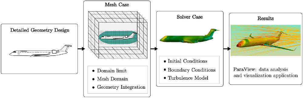
Figure 1. Overview of a ‘Simulation case’ using OpenFoam.
2.1 Bombardier CRJ700 geometry preparation
A three-dimensional model of the aircraft external geometry must be designed using a modelling software package such as Computer-Aided Design (CAD), as a watertight surface. For this study we use a CAD drawing of the CRJ700 delivered by the manufacturer Bombardier. To prepare the CAD for CFD analysis, some patches were added to fill in the spaces, for example to fill the gaps between each wing and its slat and flap surfaces. Moreover, some details were removed, such as windows and door outlines, as they created unnatural disorder at this level during mesh design.
The engines were also removed from design to avoid unnecessary computational costs. It was expected that this deletion would not have a significant impact on the lift coefficient. However, it would impact the drag coefficient computation by up to
 $\Delta {C_D}$
= 0.002 on average. This difference was estimated for the Bombardier CRJ700 from several conceptual design studies [Reference Stańkowski, MacManus, Sheaf and Christie35–Reference Raymer37]. Figure 2 shows the CRJ700 drawing used to build the aerodynamic model of the aircraft.
$\Delta {C_D}$
= 0.002 on average. This difference was estimated for the Bombardier CRJ700 from several conceptual design studies [Reference Stańkowski, MacManus, Sheaf and Christie35–Reference Raymer37]. Figure 2 shows the CRJ700 drawing used to build the aerodynamic model of the aircraft.

Figure 2. CRJ700 CAD drawing used to design the aerodynamic model.
2.2 Mesh design
From this geometry file (Fig. 2), it was necessary to design a mesh for any chosen test case. The mesh was generated by using OpenFoam tools: blockMesh and snappyHexMesh, mainly for their fully parameterised properties. However, a very wide range of parameters must be set in dictionaries that control blockMesh and snappyHexMesh applications, by making the mesh design very complex.
In order to find a good combination of blockMesh and snappyHexMesh parameters that match with the objective computing resources, we used a trial-and-errors methodology. Different mesh settings were tested, and their impact on mesh qualities and numeric solutions were analysed. As analysis of all combinations of parameters may be too exhaustive, the authors have preferred to only highlight blockMesh and snappyHexMesh pertinent settings. Indeed, these parameters settings lead to stable and accurate solutions, which were used to design the mesh.
The mesh design was mainly constrained by the available number of elements, because of the fact that our computing power was limited. Then, by using an unstructured mesh, the parameters of the mesh generators were modified with the aim to refine a particular surface or zone using a ‘specific treatment’. BlockMesh and snappyHexMesh parameters finally used to design the mesh were described using the six steps below.
2.2.1 Prepare the aircraft surface
The first step in mesh design is to provide the software with the 3D geometry of the solid (i.e. the aircraft) to be studied. Using OpenFoam, the solid can be defined from triangulated surface geometries in Stereolithography (STL) or Wavefront Object (OBJ) files formats. In this paper, an STL file was derived from the modified CAD drawing of the CRJ700 presented in Fig. 2. Using this type of file assures that all details of the geometry considered in the CAD have been considered, including the initial coordinate system.
To produce simulations with an angle-of-attack α different than zero, we decided to rotate the geometry instead of rotating the flow direction (during simulations). This solution was preferred as it kept the flow in the ‘length’ direction of the domain; more explanation is given in Subsection 2.2.4. Consequently, a STL geometry must be designed for each angle-of-attack α considered by rotating the geometry around its span axis by an α angle. The aircraft rotation was made around its aerodynamic center.
2.2.2 Generate the background mesh using OpenFoam
The second step consists in defining the domain in which the plane is studied. Following the dimensions of the STL surface, a parallelepiped domain with dimensions 44m × 44m × 70m has been set up using the blockMesh tool. According to the aircraft dimensions, the domain is 1.89 times larger than its wingspan, 7.18 times larger than its height, and 2.16 times larger than its length. The definition of the domain was a trade-off between time required for simulations and need for capturing effects due to wakes and flow deflections induced by the aircraft.
It was important to design and divide the background mesh, so that the cells respect a three-dimensional (3D) unit aspect ratio as much as possible. Consequently, a division of 44 cells were set along the vertical and lateral axis, and 70 cells along the length axis.
After generating the background mesh, the incorporation of the aircraft geometry into this block-domain has been conducted using another OpenFoam tool: snappyHexMesh (SHM). This step was illustrated on Fig. 3. Hence, at this level, the whole domain is divided by a hexahedral grid extending through the solid wall (i.e. the aircraft) within the computational domain. Integrating the STL geometry into the domain is equivalent to create a vacuum inside the geometry of the aircraft.

Figure 3. Integration of STL surface geometry in background mesh.
Consequently, the global strategy consists in refining or re-aligning cells close to solid wall, corresponding to the green zone on Fig. 3, in order to well define the outline of the aircraft. For that, we used a Cartesian-grid method; one of the advantages is that the geometry integration can be fully automated (i.e. cells division, removal of re- alignment). All operations of cells division, deletion or re-alignment of the background mesh cells around the STL geometry were made using SHM tool. There were two successive refinements steps necessary for the STL geometry integration into the background mesh, called the ‘castellated mesh’ and the ‘snapping step’.
2.2.3. Development of the castellated mesh
The castellated mesh consists in dividing and removing some cells around the aircraft using a chimera technique. As background cells were large, the highest level of refinement available (level 4) has been defined (cells were split 24 times in each direction). The smaller the cells, the better is the outline of the geometry. However, the smaller the cells, the more there are, which will require more memory and longer computational time.
It is important to mention that for any specified level of refinement, the SHM algorithm stops dividing cells if either the number of maxLocalCells or maxGlobalCells is reached. These variables correspond to the maximum number of cell attributes per parallel processor and globally, respectively. Using a system of eight processors, and 32GB of RAM memory, we have set that the maxGlobalCells can be 10 times the number of the maxLocalCells (maxLocalCells = 12,000,000). Using parallel calculation, it can happen that each processor has an unbalanced task, consequently, by using a maxGlobalCells that is slightly larger than number of processors × maxLocalCells, it could help in the uniformity of the tasks. Those maximum elements settings were the most restrictive in the mesh design as we used limited computing resources.
2.2.4. Smooth the mesh using snapping functionalities
To completely match the aircraft’s outline, it was necessary to smooth the surface of the castellated mesh using an iterative process that also been controlled through SHM tool. This process involves moving cell vertex points onto the surface geometry to remove the jagged castellated surfaces from the mesh, until mesh design reached the ‘mesh quality controls’ presented in Table 1.
Table 1. Mesh quality controls

The maximum non-orthogonality maxNonOrtho is the maximum angle tolerated to define non-orthogonal cells, while the maximum boundary skewness maxBoundarySkewness and the maximum internal skewness maxInternalSkewness are the maximum number of faces tolerated with a high skewness for a boundary face or in the internal mesh, respectively.
The most important settings that control the snapping algorithm of SHM were highlighted in the Table 2. The combination of settings that control the snapping algorithm of SHM highlighted in the Table 2 was very efficient for the CRJ700 case.
Table 2. Snap controls

2.2.5. Addition of layers around the solid to improve the boundary layer
Finally, three layers were added, with an expansion ratio of 2 for the CRJ700. Even if it is an optional step, adding layers is important to ‘standardise’cells located around the aircraft and to facilitate the wall computations.
The three layers of thickness do not exceed 8.5mm of distance from the solid. The number of layers was set to three because it was the best compromise between the cells resolution and skewness. Indeed, we noticed that adding layers could improve accuracy of solutions but induced mesh disorder and thus could cause problems for convergence. As for execution time, the mesh process took on average 8h18min using a computer equipped with eight cores and 32GB of RAM memory.
2.2.6. Final step: Check the mesh
To conclude on the mesh design process, a final verification was performed using the OpenFoam internal application checkMesh. By running checkMesh application for all the designed meshes, i.e. for angles of attack from -2 to +4deg, the user could have access to mesh qualities information.
The non-orthogonality value measured for the seven meshes was from 65.003 to 65.340deg, which was less than 70deg, and therefore these meshes could be used to perform properly flow analysis [38]. Moreover, for the skewness, a maximum value of 5.0068 was obtained for all meshes. As the smallest value is targeted to maintain the greatest accuracy possible for the simulations steps the skewness score of meshes was validated. Globally, meshes have on average 11.14 × 10+6 cells and showed an y+ value between 100 and 200, which could be considered as ‘medium’ or ‘coarse’ mesh. However, this range of y+ values is convenient to design an aerodynamic model dedicated to preliminary design analysis.
For the next simulations steps, a solver had to be chosen from among those offered by the OpenFoam toolbox. Commonly, a single solver is used. As the CRJ700 can fly up to Mach number 0.85, a compressible solver is recommended to consider compressibility effects [Reference Wilcox39]. However, many flow parameters need to be estimated by the compressible solver, mainly due to the fact that the density is not constant. In addition, the computations are often unstable and convergence is sometimes difficult to obtain, particularly when low computational resources are used (i.e. coarse or medium mesh).
To overcome this problem, an original methodology that consists of using two successive computations was developed in this paper. The first computation will use an incompressible solver (simpleFoam) that will help in the initialisation of the second computation with a compressible solver (rhoSimpleFoam). Moreover, this selection highlights the accuracy of each solver in its specific fluid domain (i.e. incompressible and compressible). This methodology allows the simulation to remain stable and increases the guarantees to achieve convergence of the compressible solver especially for the type of mesh we used (medium mesh).
The following two sub-sections (2.3 and 2.4) describe the simulations settings dedicated to simpleFoam and rhoSimpleFoam, respectively. For this purpose, given the case of an airplane flying in an environment that can be considered as uniquely incompressible, lower than Mach number 0.6, only subsection 2.3 of the methodology is necessary.
2.3. Computations using an incompressible solver: SimpleFoam
SimpleFoam tool is a solver implemented with a method that solves Navier-Stokes equations under the hypothesis of a steady and incompressible fluid. To solve the system of the RANS equations [Reference Anderson40], simpleFoam uses a well-known guess-and-correct procedure, the Semi-Implicit Method for Pressure-Linked Equations (SIMPLE) [Reference Caretto, Gosman, Patankar and Spalding41, Reference Moukalled, Mangani and Darwish42]. To avoid instability in the SIMPLE algorithm, relaxation factors were used. One set to 0.7 for pressure values and another one set to 0.3 for the velocity. Moreover, the convergence was assumed to be obtained when all residuals have reached the value of 1.10-4.
In addition to the resolution algorithm, other parameters are important to specify in order to reach a successful solution. They include the turbulence model, the finite volume solution controls, and the boundary conditions. OpenFoam offers its users the possibility of modifying all these resolution parameters in order to personalise, and thus to optimise, the computations. Hence, settings that were used for simpleFoam simulations are presented below and numbered from Sub-sections 2.3.1 to 2.3.3.
2.3.1 Turbulence model selection: Spalart-Allmaras
To compute the turbulence effects, several turbulence models were available, but two of these models are likely to be better adapted to the flow around the CRJ700 aircraft: the Spalart-Allmaras (S-A) and the
 $k - \omega $
SST (Shear Stressed Transport) turbulence model [Reference Menter43, Reference Rumsey44].
$k - \omega $
SST (Shear Stressed Transport) turbulence model [Reference Menter43, Reference Rumsey44].
As mentioned in specific bibliographical research, the S-A is an appropriate turbulence model for solving aircraft aerodynamics problems (subsonic and transonic studies) [Reference Spalart and Rumsey45]. Among its advantages, the S-A model solves the turbulence term of the NS equations with a single equation versus two equations for other models, such as the
 $k - \omega $
SST [Reference Grisval and Liauzun46].
$k - \omega $
SST [Reference Grisval and Liauzun46].
It is important to mention that in each simulation case that we performed, we used wall functions. These wall functions were used because of the fact that designed meshes were not small enough close to the wall (i.e. the aircraft), especially because of our limited computing resources. In these cases, it is common to use a wall function in order to ‘approximate’ the turbulence effects close to the wall. In order to make a model choice, we have performed some simulations using simpleFoam coupled with S-A or
 $k - \omega $
SST turbulence model (i.e. and their corresponding wall functions). Then, we have compared aerodynamic coefficients computed by models with the VRESIM data (reference), we have noticed that simulations using S-A turbulence model have converged more often than those using
$k - \omega $
SST turbulence model (i.e. and their corresponding wall functions). Then, we have compared aerodynamic coefficients computed by models with the VRESIM data (reference), we have noticed that simulations using S-A turbulence model have converged more often than those using
 $k - \omega $
SST for same initial conditions. From this observation, we assumed that the S-A model offered a larger stability in the computation of aerodynamic coefficients, certainly due to its one turbulence-equation. However, we observed that with accurate initial conditions (closest to the solution), simulations using
$k - \omega $
SST for same initial conditions. From this observation, we assumed that the S-A model offered a larger stability in the computation of aerodynamic coefficients, certainly due to its one turbulence-equation. However, we observed that with accurate initial conditions (closest to the solution), simulations using
 $k - \omega $
SST turbulence model provided the aerodynamic coefficients closest to the reference data, as shown on Fig. 4.
$k - \omega $
SST turbulence model provided the aerodynamic coefficients closest to the reference data, as shown on Fig. 4.

Figure 4. Overview of the Turbulence Model Influence (
 $\alpha $
= 0 deg).
$\alpha $
= 0 deg).
Figure 4 shows a comparison of the forces values obtained with simpleFoam: those obtained with the Spalart-Allmaras (S-A) turbulence model in ‘blue’, with the
 $k - \omega $
SST model in ‘purple’, and with no turbulence model in ‘pink’. The normalised lift and drag forces obtained for the three models are displayed in Fig. 4(a) and (b), respectively, and compared with their normalised reference forces obtained from the VRESIM (in ‘black’). Simulations were performed for different Mach numbers from M0.31 to M0.79 and for a fixed angle-of-attack
$k - \omega $
SST model in ‘purple’, and with no turbulence model in ‘pink’. The normalised lift and drag forces obtained for the three models are displayed in Fig. 4(a) and (b), respectively, and compared with their normalised reference forces obtained from the VRESIM (in ‘black’). Simulations were performed for different Mach numbers from M0.31 to M0.79 and for a fixed angle-of-attack
 $\alpha $
= 0 deg.
$\alpha $
= 0 deg.
For the lift prediction (Fig. 4(a)), it could be observed that both the S-A and
 $k - \omega $
SST turbulence models give a good approximation of the reference lift value for all Mach numbers (from M0.31 to M0.79). The
$k - \omega $
SST turbulence models give a good approximation of the reference lift value for all Mach numbers (from M0.31 to M0.79). The
 $k - \omega $
SST turbulence model simulation gives the closest lift forces results to their reference values for Mach numbers M0.31–M0.54. For Mach numbers higher than 0.6, the trend changes and simulations using the S-A turbulence model give closer lift values to their reference values than the
$k - \omega $
SST turbulence model simulation gives the closest lift forces results to their reference values for Mach numbers M0.31–M0.54. For Mach numbers higher than 0.6, the trend changes and simulations using the S-A turbulence model give closer lift values to their reference values than the
 $k - \omega $
SST turbulence model. It is important to remember that simpleFoam is a solver that does not take into account the fluid compressibility; therefore, it is normal to obtain for this solver, large errors for Mach numbers higher than 0.6.
$k - \omega $
SST turbulence model. It is important to remember that simpleFoam is a solver that does not take into account the fluid compressibility; therefore, it is normal to obtain for this solver, large errors for Mach numbers higher than 0.6.
The effect of the presence or not of a turbulence model is visible on the drag force comparison (Fig. 4(b)). For simulations made with no turbulence model (in ‘pink’), the drag force estimated by simpleFoam is practically half that of the reference force. The lift force is less affected by the turbulence model selection. From these observations, it seems obvious that a turbulence model must be defined, as expected, to predict the aerodynamic forces of the CRJ700 with a very good accuracy.
The main effects affecting the drag force are: the shape (predominant in blunt bodies), friction (significant in streamlined bodies) and induced drag (noticeable only when there is a lift). Concerning the drag prediction (Fig. 4(b)), a remark similar to that for the lift prediction can be made. The
 $k - \omega $
SST turbulence model gives a closer drag value to its reference value than the S-A model. In fact, for Mach numbers M0.31–M0.54, the
$k - \omega $
SST turbulence model gives a closer drag value to its reference value than the S-A model. In fact, for Mach numbers M0.31–M0.54, the
 $k - \omega $
SST turbulence model over-estimated the drag force while the S-A turbulence model under-estimates it. The overestimation could be explained by the fact that the engine design had been removed from the CAD. This overestimation trend changed for Mach numbers M0.66 and M0.79, and it could be explained by the fact that simpleFoam did not compute compressibility effects, and thus simulations in this range of Mach numbers were not enough reliable (for simpleFoam). For this reason, it was expected that for Mach numbers higher than 0.6, simulations converged toward a solution that was far away from the reference (real) one due to the incompressibility assumption.
$k - \omega $
SST turbulence model over-estimated the drag force while the S-A turbulence model under-estimates it. The overestimation could be explained by the fact that the engine design had been removed from the CAD. This overestimation trend changed for Mach numbers M0.66 and M0.79, and it could be explained by the fact that simpleFoam did not compute compressibility effects, and thus simulations in this range of Mach numbers were not enough reliable (for simpleFoam). For this reason, it was expected that for Mach numbers higher than 0.6, simulations converged toward a solution that was far away from the reference (real) one due to the incompressibility assumption.
Based on the observations made for Fig. 4, simpleFoam simulations for the CRJ700 were performed with the S-A turbulence model (while solution stability is a priority). For compressible simulations with rhoSimpleFoam, the
 $k - \omega $
SST turbulence model was preferred in order to achieve a better step of accuracy (while solution stability was maintained due to its initialisation, that will be explained in Section 2.4).
$k - \omega $
SST turbulence model was preferred in order to achieve a better step of accuracy (while solution stability was maintained due to its initialisation, that will be explained in Section 2.4).
2.3.2 Initial and boundary conditions
The SIMPLE procedure is a very robust method, but it exhibits a quite low asymptotic convergence rate [Reference Moukalled, Mangani and Darwish42]. In order to remain within an acceptable convergence rate, it is important to define the initial and boundary conditions for the flow parameters with enough accuracy. Using simpleFoam, two parameters must be initialised: the kinematic pressure p and the velocity magnitude and direction U. If a turbulence model is desired for the simulation, its parameters need to be initialised as well (e.g. there are two parameters for an S-A model).
For the CRJ700, simpleFoam simulations with a freestream kinematic pressure at the inlet and at the outlet of the domain were set with a value p . To initialise each case, the kinematic pressure p (in m2/s2) was computed using Equation (1), where P and
 $\rho $
are the pressure and the air density, respectively, obtained from International Standard Atmosphere (ISA) equations at a given altitude. On the surface of the aircraft, the kinematic pressure was defined using a zero gradient of kinematic pressure.
$\rho $
are the pressure and the air density, respectively, obtained from International Standard Atmosphere (ISA) equations at a given altitude. On the surface of the aircraft, the kinematic pressure was defined using a zero gradient of kinematic pressure.
 \begin{align}{p^{\left( 0 \right)}} = \frac{P}{\rho }\end{align}
The velocity was defined as freestream flow for the inlet and the outlet faces. The magnitude of the flow velocity was always fully defined in the length direction because the mesh was already rotated according to the angle-of-attack
 $\alpha $
. The value of the flow speed (in m/s) was determined from the imposed Mach number M, and the speed of sound at a given altitude using Equation (2).
$\alpha $
. The value of the flow speed (in m/s) was determined from the imposed Mach number M, and the speed of sound at a given altitude using Equation (2).
 \begin{align}{U^{\left( 0 \right)}} = U_z^{\left( 0 \right)} = M \times a\end{align}
As the Spalart-Allmaras turbulence model introduces two parameters —the kinematic viscosity
 $\nu $
and the turbulent kinematic viscosity
$\nu $
and the turbulent kinematic viscosity
 $\tilde \nu $
—it is important to set initial conditions for these values. Both of these parameters are introduced as freestream types for each face of the domain. Values of
$\tilde \nu $
—it is important to set initial conditions for these values. Both of these parameters are introduced as freestream types for each face of the domain. Values of
 $\nu $
and
$\nu $
and
 $\tilde \nu $
(in m2/s) were initialised using Equation (3) with the dynamic viscosity
$\tilde \nu $
(in m2/s) were initialised using Equation (3) with the dynamic viscosity
 $\mu $
and the density
$\mu $
and the density
 $\rho $
known at a given altitude.
$\rho $
known at a given altitude.
 \begin{align}{\nu ^{\left( 0 \right)}} = {\tilde \nu ^{\left( 0 \right)}} = \frac{\mu }{\rho }\end{align}
For the aircraft boundary modelling, a wall function was set as nutUSpaldingWallFunction for both
 $\nu $
and
$\nu $
and
 $\tilde \nu $
parameters. This wall function modified the velocity profile close to the wall (i.e. the aircraft) by taking into account the Spalding equation [Reference Launder and Spalding47, Reference Fangqing48]. The use of a wall function approach allows the user to impose the flow field close to the wall without having to use a large number of mesh cells, which is much more efficient from the perspective of memory use. As a reminder, y+ values of designed meshes were found to be between 100 and 200 and OpenFoam advised to use these wall functions for high Reynolds numbers conditions, which is the case of targeted simulations [49].
$\tilde \nu $
parameters. This wall function modified the velocity profile close to the wall (i.e. the aircraft) by taking into account the Spalding equation [Reference Launder and Spalding47, Reference Fangqing48]. The use of a wall function approach allows the user to impose the flow field close to the wall without having to use a large number of mesh cells, which is much more efficient from the perspective of memory use. As a reminder, y+ values of designed meshes were found to be between 100 and 200 and OpenFoam advised to use these wall functions for high Reynolds numbers conditions, which is the case of targeted simulations [49].
2.3.3 Solution controls
The solution computed by the solver is controlled by two important dictionaries: fvSolution and fvScheme. Both dictionaries characterise how the user wants to integrate flow properties between cells, and, if an accurate or a stable mathematical treatment is preferred for the resolution.
The fvSolution dictionary helps the user to set how the iterative process should work by specifying the linear solver that OpenFoam needs to linearise each equation being solved. The pressure matrix is symmetrical, consequently, the Geometric-Algebraic Multi Grid (GAMG) solver was chosen, along with a GaussSeidel run-time ‘smoother’ to reach the tolerance fixed at 1.10-6 for the study (relative tolerance of 0.01). The GAMG has a good reputation for this kind of resolution; it offers rapid convergence and is the most stable solver available [50].
To compute the velocity solution, SmoothSolver, an iterative solver, was selected. Indeed, SmoothSolver is usually used to solve symmetric and asymmetric matrices (the velocity here is an asymmetric matrix). SmoothSolver was coupled with the run-time ‘smoother’ GaussSeidel, set with a two ‘sweeps’ to reach the tolerance, fixed at 1.10-6 (relative tolerance of 0.1 on residuals). The kinematic turbulent viscosity (i.e.
 $\tilde \nu $
) was set with the same settings.
$\tilde \nu $
) was set with the same settings.
The fvScheme dictionary allows the user to define the properties linked to the finite volume approach that need to be considered. These properties are linked to the divergence theory [Reference Moukalled, Mangani and Darwish42]. In this study, all properties were set by default, except the divergence scheme criteria, which were set using a bounded Gauss linear upwind method (i.e. second-order bounded). This type of method was selected because of its offered accuracy, even if it may lead to a small oscillatory behaviour (along computation iterations).
Most settings were kept by default, as they were already specified for our type of computation. For example, the Laplacian scheme was set by default using a corrected linear Gauss method. This setting is generally better for meshes that have a nonlinear grading (i.e. with an expansion ratio not equal to 1) and that are non-orthogonal. Even if mesh cells in this study have been defined using same size, the refinement operation creates very small-volume cells around the aircraft while background cells remain within a big volume. At computation level, the layout of our mesh could be equivalent to a nonlinear mesh grading. Consequently, using this type of scheme to work with a Laplacian scheme is practical.
Finally, simpleFoam simulations were carried out with the same computer setup as for the mesh (eight cores and 32GB of RAM memory). Therefore, computations were also realised using ‘parallel decomposition’. On average, a simulation with simpleFoam took 14 hours and 21 minutes, with a minimum and a maximum time of execution of 12h29 and 16h54, respectively. This computation time appears to be totally acceptable, depending on the hardware used and the expected level of accuracy.
In the case in which a compressible simulation of the fluid was required (i.e. for an aircraft flying higher than M0.3), the last part of the methodology was performed in order to obtain accurate results. Therefore, in order to account for the compressibility effects that appear in the transonic fluid domain, a second computation using a compressible solver is recommended. In this paper, the compressible solver used is rhoSimpleFoam.
2.4 Computations using a compressible solver: rhoSimpleFoam
The rhoSimpleFoam is a pressure-based solver that uses the same resolution process as the simpleFoam, which is the SIMPLE algorithm. However, rhoSimpleFoam solves the compressible Navier-Stokes equations in their conservative form.
2.4.1 Initials and boundaries conditions
Due to the large number of parameters that must be estimated by the rhoSimpleFoam solver, the initialisation of this solver was optimised using the converged solution obtained by the incompressible flow solver simpleFoam. Using this process allows to conserve the stability of the incompressible solver and therefore, increases the guarantees to achieve convergence for compressible simulations.
The last iteration of computation realised using the incompressible solver simpleFoam provides a stable solution of the kinematic pressure
 ${p^{\left( {end} \right)}}$
, the velocity
${p^{\left( {end} \right)}}$
, the velocity
 ${U^{\left( {end} \right)}}$
, the kinematic flux
${U^{\left( {end} \right)}}$
, the kinematic flux
 ${\phi ^{\left( {end} \right)}}$
and the turbulence variables
${\phi ^{\left( {end} \right)}}$
and the turbulence variables
 ${\nu ^{\left( {end} \right)}}$
and
${\nu ^{\left( {end} \right)}}$
and
 ${\tilde \nu ^{\left( {end} \right)}}$
. In order to initialise the compressible flow solver rhoSimpleFoam, it is necessary to provide the pressure P, the velocity U and the turbulence parameters. This initialisation requires to manage the solution of
${\tilde \nu ^{\left( {end} \right)}}$
. In order to initialise the compressible flow solver rhoSimpleFoam, it is necessary to provide the pressure P, the velocity U and the turbulence parameters. This initialisation requires to manage the solution of
 ${p^{\left( {end} \right)}}$
(in m2/s2) obtained from simpleFoam in order to include the density value and define P (in kg/m/s2) for rhoSimpleFoam, using Equation (4).
${p^{\left( {end} \right)}}$
(in m2/s2) obtained from simpleFoam in order to include the density value and define P (in kg/m/s2) for rhoSimpleFoam, using Equation (4).
 \begin{align}{P^{\left( 0 \right)}} = {p^{\left( {end} \right)}} \times \rho \end{align}
Concerning the velocity U, no modifications are required, so that the solution file obtained from simpleFoam can be placed directly in the rhoSimpleFoam initialisation folder.
In addition to the pressure and velocity, compressible simulations using rhoSimpleFoam need to be initialised using the temperature T. Therefore, for the CRJ700 simulations, the walls of the domain (using inletOutlet boundary condition) were initialised using the temperature value T (in Kelvin) calculated from the ISA atmosphere for a specific altitude. On the surface of the aircraft, the temperature was defined using a zeroGradient boundary condition.
2.4.2 Turbulence model selection:
$k - \omega $
SST (shear stressed transport)

From the observation made from Fig. 4, simulations performed using a
 $k - \omega $
SST turbulence model have provided the closest aerodynamic coefficients with respect to the reference (VRESIM) when the solution is precisely initialised. Because of the fact that rhoSimpleFoam simulations were initialised using the converged field solution provided by simpleFoam, the
$k - \omega $
SST turbulence model have provided the closest aerodynamic coefficients with respect to the reference (VRESIM) when the solution is precisely initialised. Because of the fact that rhoSimpleFoam simulations were initialised using the converged field solution provided by simpleFoam, the
 $k - \omega $
SST turbulence model was preferred to be used for rhoSimpleFoam simulations.
$k - \omega $
SST turbulence model was preferred to be used for rhoSimpleFoam simulations.
The
 $k - \omega $
SST turbulence model is governed by two transport equations, one equation for the turbulent kinetic energy k and another equation for the specific turbulence rate of dissipation
$k - \omega $
SST turbulence model is governed by two transport equations, one equation for the turbulent kinetic energy k and another equation for the specific turbulence rate of dissipation
 $\omega $
. The turbulence model equations are not developed in this paper because it is not within the scope of this study. The version of the
$\omega $
. The turbulence model equations are not developed in this paper because it is not within the scope of this study. The version of the
 $k - \omega $
SST turbulence model implemented in OpenFoam is based on Ref. Reference Menter, Kuntz and Langtry51, and the constants dedicated to the model are detailed in the OpenFoam manual [49].
$k - \omega $
SST turbulence model implemented in OpenFoam is based on Ref. Reference Menter, Kuntz and Langtry51, and the constants dedicated to the model are detailed in the OpenFoam manual [49].
For rhoSimpleFoam simulations, wall functions kqRWallFunction and omegaWallFunction were used as boundaries conditions at the aircraft level for turbulence parameters k and
 $\omega $
, respectively [Reference Moukalled, Mangani and Darwish42, 49]. This type of function computes k and
$\omega $
, respectively [Reference Moukalled, Mangani and Darwish42, 49]. This type of function computes k and
 $\omega $
values from a universal profile, close to the solid (i.e. the aircraft), even if the mesh is not extremely thin at this level. Side boundaries of the domain were set using a slip type for turbulence parameters. As for the Spalding wall function, the OpenFoam manual advised to use them for high Reynold numbers, which is convenient for our cases [49].
$\omega $
values from a universal profile, close to the solid (i.e. the aircraft), even if the mesh is not extremely thin at this level. Side boundaries of the domain were set using a slip type for turbulence parameters. As for the Spalding wall function, the OpenFoam manual advised to use them for high Reynold numbers, which is convenient for our cases [49].
Turbulence model (
 $k - \omega $
SST) parameters, k and
$k - \omega $
SST) parameters, k and
 $\omega $
were initialised at the inlet and at the outlet. Due to the complexity of these parameters, they are usually unknown however, different equations could give an approximation of their values [Reference Moukalled, Mangani and Darwish42]. In this study, the initial values of k (in m2/s2) and
$\omega $
were initialised at the inlet and at the outlet. Due to the complexity of these parameters, they are usually unknown however, different equations could give an approximation of their values [Reference Moukalled, Mangani and Darwish42]. In this study, the initial values of k (in m2/s2) and
 $\omega $
(in /s) were computed from Equations (5) and (6), respectively.
$\omega $
(in /s) were computed from Equations (5) and (6), respectively.
 \begin{align}{k^{\left( 0 \right)}} = {\left( {\frac{v}{l}} \right)^2}\end{align}
 \begin{align}{\omega ^{\left( 0 \right)}} = \sqrt {\frac{k}{l}} \end{align}
where
 $\nu $
is the kinematic viscosity and l is the reference length. The length of the mean aerodynamic chord of the CRJ700 was used for its reference length l.
$\nu $
is the kinematic viscosity and l is the reference length. The length of the mean aerodynamic chord of the CRJ700 was used for its reference length l.
2.4.3 Solution controls
Solution controls used to set rhoSimpleFoam solver simulations were globally the same of those that were used for simpleFoam solver simulations. However, rhoSimpleFoam is a compressible solver that needs to deal with temperature and energy variables (that were neglected for incompressible simulations). Therefore, to predict the onset of shocks, it was necessary to select a temperature dependent transport model. For its general applications, the Sutherland viscosity model has been set in the thermophysicalProperties dictionary using the default constants [Reference White52]. Using the Sutherland Equation (7), the dynamic viscosity
 $\mu $
(in kg/m/s1) is estimated from the temperature T, and the Sutherland constants are
$\mu $
(in kg/m/s1) is estimated from the temperature T, and the Sutherland constants are
 ${A_s}$
= 1.458.10-6 and
${A_s}$
= 1.458.10-6 and
 ${T_s}$
= 110.4°K for the air.
${T_s}$
= 110.4°K for the air.
 \begin{align}\left( {{\rm{Sutherland\ viscosity\ Model}}} \right):\mu = \frac{{{A_s}\sqrt T }}{{1 + \frac{{{T_s}}}{T}}}\end{align}
Furthermore, additional information was added to fvSolution and fvScheme dictionaries due to the compressible solver (such as parameters related to energy or
 $k - \omega $
SST turbulence model).
$k - \omega $
SST turbulence model).
For the fvSolution dictionary, the same settings as those used to compute the velocity solution with the simpleFoam solver (i.e. the SmoothSolver solver coupled with GaussSeidel run-time ‘Smoother’) were used to compute the solutions for k,
 $\omega $
, and the energy e.
$\omega $
, and the energy e.
The turbulence divergence scheme was expressed with a Gauss upwind method. This kind of numerical method of resolution is also called a ‘forward’ integral method [Reference Moukalled, Mangani and Darwish42]. Computing the next iterations using the previous ones is a very efficient and economical computation method. Most interesting aspects with this method is the compromise between speed of resolution and stability. This numerical method of resolution (Gauss upwind) has also been used to compute the divergence control criteria of energy parameters.
The complete simulation case for rhoSimpleFoam was designed utilising all these specifications. Simulations were done for different flight conditions in order to cover the whole CRJ700 flight envelope. RhoSimpleFoam simulations were also accomplished with a computer with a limited capacity (eight cores and 32GB of RAM memory). To save execution time, computations were parallelised on the eight processors of the computer using the ‘Scotch’ method [Reference Chevalier and Pellegrini53]. On average, the 35 computations using the rhoSimpleFoam solver were processed 2 hours faster than those processed with the simpleFoam solver; however, the convergence was not reached ‘directly’ in some cases because of the fact that the initial state was too far from the solution (due to the compressibility effects), and thus, the solution had a slightly oscillatory trend, and the computation time went up to 30 hours until the solution would reach a stable state.
2.5 Force estimations and post-treatment
Aerodynamic forces and moments acting on the CRJ700 were computed with simpleFoam or rhoSimpleFoam by use of an internal function forcesCompressible programmed in OpenFoam software. The forces and moments presented as results were obtained from the last computation iteration by adding the pressure and viscous aspects together. The aerodynamic coefficients of lift
 ${C_L}$
, drag
${C_L}$
, drag
 ${C_D}$
were computed from lift L and drag D forces using Equation (8), and pitching moment coefficient
${C_D}$
were computed from lift L and drag D forces using Equation (8), and pitching moment coefficient
 ${C_{{m_y}}}$
were computed using pitching moments M
y
according to Equation (9):
${C_{{m_y}}}$
were computed using pitching moments M
y
according to Equation (9):
 \begin{align}{C_{L,D}} = \frac{{2 \times \left[ {F_{L,D}^{\left( {end} \right)}\left( {{\rm{pressure}}} \right) + F_{L,D}^{\left( {end} \right)}\left( {{\rm{viscous}}} \right)} \right]}}{{\rho .S.{V^2}}}\end{align}
 \begin{align}{C_{{m_y}}} = \frac{{2 \times \left[ {M_y^{\left( {end} \right)}\left( {{\rm{pressure}}} \right) + M_y^{\left( {end} \right)}\left( {{\rm{viscous}}} \right)} \right]}}{{\bar c.\rho .S.{V^2}}}\end{align}
where
 $\rho $
is the air density for the selected altitude (following ISA atmospheric model), S is the wing area of the aircraft, V is the aircraft True Air Speed (TAS) (i.e. the fluid speed in the simulation context) and
$\rho $
is the air density for the selected altitude (following ISA atmospheric model), S is the wing area of the aircraft, V is the aircraft True Air Speed (TAS) (i.e. the fluid speed in the simulation context) and
 $\bar c$
is the mean aerodynamic chord of the aircraft wing.
$\bar c$
is the mean aerodynamic chord of the aircraft wing.
3.0 Simulation results
To give an overview of the aerodynamic model’s validity, CFD simulations were performed for the five combinations of Altitude-Mach that are the most representative for the CRJ700. The combinations are shown in Table 3. These flight conditions were selected after performed several flight plans using the VRESIM flight simulator of the CRJ700.
Table 3. Flight conditions selected to test the aerodynamic model

3.1. Convergence study
To demonstrate the stability of the solutions given by the simpleFoam solver, Fig. 5 shows the residual convergence obtained for all the cases evaluated. This figure presents the simulation cases using two colors: ‘magenta’ for cases when the angle-of-attack is equal to zero, and the ‘blue’ for cases when angles of attack within the range -2 to 4deg, except zero. Figure 5 shows that the residual convergence criteria of 10-4 (a ‘dashed red’ line) is not reached at the same time, as meeting this goal depends on the nature of the parameter (pressure or velocity) and its axis (x, y or z). The z-velocity is the parameter that converges the quickest as seen on Fig. 5 (d). In this study, the z-axis is located along the wing plan; this observation could signify that the fluid behaviour is easier to predict in the axis that is not directly affected by the flow direction. All the other parameters have residuals that reached convergence after 1,000 iterations of computations.

Figure 5. Residual convergence of pressure and velocity obtained for simpleFoam computations.
Another observation can be made concerning the dependency of the angle-of-attack in residual convergence. Indeed, cases where angles of attack are equal to zero converged sooner than those for other angles of attack. This could be explained by the alignment of the aircraft in the mesh domain, as the aircraft is not perfectly aligned with the length axis (x- axis) for angles of attack that are not zero, which renders the computation more difficult and less stable. Consequently, convergence is reached a bit later for these cases than for cases where angles of attack are zero.
Figure 6 shows the residual convergence achieved with rhoSimpleFoam solver computations. Contrary to the observations in Fig. 5 for simpleFoam solver computations, straight convergences can be observed here for both the pressure and the velocity. The convergence is especially straight at the beginning, due to the initialisation of the solver using the previous computation results that were performed with simpleFoam. This initialisation could also explain why fewer than 1,000 iterations are required to reach convergence with rhoSimpleFoam than with simpleFoam (where twice as many iterations are required to observe convergence in all cases). However, the pressure residuals are also the ‘limiting condition of convergence’ for rhoSimpleFoam computations, as the velocity in each direction has already reached the convergence criteria.

Figure 6. Residual convergence for rhoSimpleFoam computations.
This first overview of the convergence results reveals that there are flight conditions that allow the simulation to find a convergence more quickly than others. For instance, simpleFoam simulations with an angle-of-attack of 0deg converged faster than those for other angles of attack, whatever the Mach number selected. Concerning the rhoSimpleFoam simulations, solutions converged rapidly (in less than 1,000 iterations), as they were initialised with last iteration results of the simpleFoam computation.
3.2 Comparison of the lift coefficients (
${\textbf{{C}}_{\textbf{{L}}}}$
) between the aerodynamic models and the reference (VRESIM)

The lift coefficient
 $({C_L}$
) is the first aerodynamic parameter analysed and compared. The lift coefficient values with angles of attack from -2 to 4deg were computed and compared at Mach number values from 0.31 to 0.54 (low values) and at 0.66 and 0.79 (high values). The results obtained with the simpleFoam model (in ‘pink’), and the rhoSimpleFoam model (in ‘purple’) were compared to the reference (provided by VRESIM) values (in ‘black), in Fig. 7 (for low Mach values) and Fig. 8 (for high Mach values). It is important to specify that for confidentiality reasons, the y-axes of these graphs have been hidden. We also want to mention that simpleFoam results were presented in the paper as ‘intermediary’ results obtained through the methodology (until reaching rhoSimpleFoam results). Consequently, it was out of scope to improve simpleFoam results. However, according to the level of accuracy required, and the flight conditions that the reader want to simulate, results provided by simpleFoam, could be corrected using a Prandtl-Glauert equation to reach a ‘convenient’ level of accuracy (and low computational resources).
$({C_L}$
) is the first aerodynamic parameter analysed and compared. The lift coefficient values with angles of attack from -2 to 4deg were computed and compared at Mach number values from 0.31 to 0.54 (low values) and at 0.66 and 0.79 (high values). The results obtained with the simpleFoam model (in ‘pink’), and the rhoSimpleFoam model (in ‘purple’) were compared to the reference (provided by VRESIM) values (in ‘black), in Fig. 7 (for low Mach values) and Fig. 8 (for high Mach values). It is important to specify that for confidentiality reasons, the y-axes of these graphs have been hidden. We also want to mention that simpleFoam results were presented in the paper as ‘intermediary’ results obtained through the methodology (until reaching rhoSimpleFoam results). Consequently, it was out of scope to improve simpleFoam results. However, according to the level of accuracy required, and the flight conditions that the reader want to simulate, results provided by simpleFoam, could be corrected using a Prandtl-Glauert equation to reach a ‘convenient’ level of accuracy (and low computational resources).

Figure 7. Lift coefficient comparison for low Mach numbers value.

Figure 8. Lift coefficient comparison for high Mach numbers values.
The lift coefficient variation with the angle-of-attack for low Mach numbers, typically M0.31, 0.45 and M0.54, were displayed in Fig. 7(a), (b) and (c), respectively. For the whole range of angles of attack, from -2.0 to +4.0deg, it could be assumed that the lift varies linearly (before stall). As a consequence, the lift slope obtained by use of simpleFoam model was close to the reference lift slope (given by the VRESIM) for Mach numbers M0.31 and M0.45. However, the rhoSimpleFoam solver model gave results closer to the reference ones Mach conditions presented on Fig. 7 than simpleFoam model. It has been therefore shown that the incompressible model (simpleFoam) has not given representative results for Mach numbers higher than M0.45.
A maximum absolute error of 0.020 was obtained for this rhoSimpleFoam model. Similar results were obtained for the simpleFoam model, except for negative angles of attack, where the lift coefficient was overestimated with an absolute error of 0.022. It is important to specify that a 0.022 error margin is acceptable for an aerodynamic model to be used in the preliminary design phases.
The lift coefficient comparisons versus the angle-of-attack for two high Mach number values, M0.66 and M0.79, are displayed in Fig. 8(a) and (b), respectively. In this Mach number range, the effects of compressibility are no longer negligible. Indeed, this can be easily observed from the results obtained with the simpleFoam solver, shown in ‘pink’. Despite the incompressibility hypothesis, the simpleFoam solver offered acceptable results for M0.66, with a maximum absolute error of 0.085 observed for the angle-of-attack of 4deg. However, for M0.79, simpleFoam converges towards solutions that are very different to reference values (with a margin of error higher than 0.1). Consequently, as expected, simpleFoam could be considered as less optimal than rhoSimpleFoam for high Mach value of M0.66 and M0.79.
Meanwhile, the compressible solver, rhoSimpleFoam, does account for the compressible effects of the fluid, and therefore its results match closely those of the VRESIM reference. For angles of attack from -1 to 3deg, rhoSimpleFoam can predict the CRJ700 VRESIM lift coefficient within a maximum margin error of 0.035.
3.3 Comparison of the drag coefficients (
${\textbf{{C}}_{\textbf{{D}}}}$
) between the aerodynamic models and the reference (VRESIM)

Similarly, drag coefficients obtained from simulations performed using simpleFoam and rhoSimpleFoam solvers were compared to those of the reference VRESIM according to the angle-of-attack. These results are presented for five Mach numbers values in Figs. 9 and 10. Comparisons for low Mach number (from 0.31 to 0.54) are displayed in Fig. 9(a), (b) and (c), and those for high Mach number (M0.66 and M0.79) are presented in Fig. 10(a) and (b).

Figure 9. Drag coefficient comparison for low Mach numbers values.

Figure 10. Drag coefficient comparison for high Mach numbers values.
Figure 9(a) and (b) show that the simpleFoam solver can predict the drag coefficients for angles of attack from -2.0 to 4.0deg with a maximum absolute error of 0.0022 with respect to VRESIM values, while the compressible solver, rhoSimpleFoam, can predict the drag coefficient with a maximum absolute error of 0.0006 with respect to the reference (VRESIM). Thus, for Mach numbers 0.31 and 0.45, it was observed that rhoSimpleFoam was 3.5 times better than simpleFoam to predict drag coefficients.
For Mach number 0.54, on Fig. 9(c), it was observed that maximum absolute errors for both solvers were slightly higher, especially for the angle-of-attack of 4deg (0.004 for rhoSimpleFoam and 0.0015 for simpleFoam) than those observed for lower Mach numbers on Fig. 9(a) and (b). This observation could be explained by the fact that the angle-of-attack could increase the compressibility effect. Because Mach number 0.54 is situated at the limit of compressibility, and simpleFoam does not consider compressibility effects, it was expected that the results provided by this solver could be less representative for these flight conditions. For the second solver, rhoSimpleFoam, a range of errors close to 0.0015, could be explained by the fact that engines design was removed from the CAD model. Indeed, in the literature, it was found that this removal could affect the drag coefficient up to 0.002 according to empirical techniques [Reference Stańkowski, MacManus, Sheaf and Christie35, Reference Lee and Pendergraft36]. In consequence, results obtained using rhoSimpleFoam are acceptable.
An observation similar to those made for the lift coefficient comparison for high values of Mach can also be made for the drag coefficient comparison for same Mach numbers. Indeed, the compressibility effect cannot be neglected for Mach numbers M0.66 and M0.79, and thus the simpleFoam solver is not really appropriate to use for these flight conditions. However, for M0.66 and angles of attack very close to 0deg, the simpleFoam solver delivered drag coefficients with less than 0.002 of absolute error, which indicates that it performs well.
Meanwhile, the compressible solver (rhoSimpleFoam) estimated the drag coefficient of the CRJ700, within a maximum error of 0.0015 with respect to the reference (VRESIM), except for angles of attack of 0 and 4deg at Mach number M0.79 (Fig. 10(b)) and for 4deg at M0.66 (Fig. 10(a)) where the maximum absolute error is less than 0.0026. This exception appears to be due to a small ‘deviation’ in the convergence, a situation that has occurred occasionally for simulations with rhoSimpleFoam. In this case, the convergence is quite oscillatory and sometimes not enough iterations are allowed for the solver to converge within the imposed minimum residual limit (10-4). Finally, to overcome this situation, the simulation should be completed using close to 100 more iterations.
It is important to notice that a maximum absolute error of 0.0015 for the drag coefficient prediction is a small error as the model aims to be used for preliminary design studies. Thus, the mesh of the model was designed as ‘coarse’ as possible due to the limited computing resources. Moreover, this level of error is largely acceptable as some assumptions were initially made, as for instance, the engines removal from the CAD drawing.
3.4 Comparison of the pitching moment coefficients
${\textbf{{C}}_{\textbf{{M}}}}_{\textbf{{y}}}$
between the models and the reference (VRESIM)

Lastly, the pitching moment coefficients computed by OpenFoam solvers were compared to those of the reference (VRESIM) versus lift coefficients. It is important to mention that the pitching moment coefficient is generally very difficult to predict from aerodynamic perspective, because it is very sensitive to the aerodynamic center position. To avoid the projection of forces and moments from an axis to another one, the same aerodynamic center coordinates were set for the CAD drawing (the design of the *.STL files for each angle-of-attack), and for the OpenFoam force function of computation. Pitching moment coefficient versus the lift coefficient were compared for low Mach numbers (M0.31–M0.54) on Fig. 11(a), (b) and (c), and for Mach numbers M0.66 and M0.79 on Fig. 12 (a) and (b), respectively.

Figure 11. C My = f(C L ) comparison for low Mach numbers values.

Figure 12. C My = f(C L ) comparison for high Mach numbers values.
Globally, the pitching moment coefficient is less well-estimated than the lift and drag coefficients. However, both the simpleFoam and rhoSimpleFoam computations found pitching moment coefficients with a maximum absolute error of 0.017 of error, except for negative angles of attack (where maximum absolute errors are close to 0.072). For positive angles of attack (i.e. 0–4deg), the rhoSimpleFoam solver well estimated the pitching moment coefficient with a maximum absolute error of 0.017 from the reference.
The difficulty involved in predicting the pitching moment coefficients for negative angles of attack could be related again to the fact that the engines of the CRJ700 were removed from CAD drawing for the aerodynamic computations. However, normally a part of the total pitching moment of the aircraft is due to the engines’ geometry (and this aspect was considered in the VRESIM values).
The engine part of the total pitching moment depends evidently on the engine geometry and on the aircraft’s angle-of-attack. Indeed, the engine lift and drag forces generated a moment at the aerodynamic center. Because of the fact that the engines attachments to the fuselage rear has a certain fixed pitch angle, the absence of engines design in the simulations mainly impacts the analysis results for negative angles of attack.
Similar observations can be made for Mach numbers M0.66 and M0.79. From Fig. 12(b), it seems that the compressible solver rhoSimpleFoam has some difficulties to match the reference (VRESIM), but the incompressible solver simpleFoam did not, which was surprising. Despite of the special shape of the rhoSimpleFoam results, the pitching moment coefficients were fairly well-estimated, with a maximum absolute error of 0.015 for positive angles of attack. The simpleFoam solver estimated the pitching moment coefficients with a slightly larger error (0.035 of error from the VRESIM). This last observation was expected, as simpleFoam is an incompressible solver, and thus this hypothesis could not be applied for cases where Mach numbers is over M0.6 [Reference Friedlander and Serre54].
3.5 Results summary obtained using the compressible solver rhoSimplefoam
In order to summarise results obtained for the compressible solver rhoSimpleFoam, a statistical study was finally performed. Thus, for the three longitudinal aerodynamic coefficients (i.e. C L , C D and C My ), absolute errors recorded for all flight conditions tested previously have been displayed in Fig. 13(a), (b) and (c), respectively.

Figure 13. Statistical study concerning rhoSimpleFoam prediction errors over the 35 flight conditions.
Errors are displayed following the x-axis, while the y-axis is dedicated to show the number of instances. The bars show the number of predicted flight conditions with the in corresponding absolute errors displayed on the x-axis. The red curve describes the normal distribution of these values. The normal distribution shape allows to define if the distribution of errors is narrow or wide.
On Fig. 13(a), it was observed that the solver rhoSimpleFoam, was able to predict the lift coefficient with less than 0.05 of absolute error from VRESIM values, for 34 flight conditions (over 35). Globally, rhoSimpleFoam has predicted the lift coefficient with an average error of -0.007 (top of the red curve) and a standard deviation of ±0.045. This aspect means that rhoSimpleFoam was able to predict lift coefficient of the Bombardier CRJ700 within a margin error of -0.007 ± 0.045 in 95% of cases.
On Fig. 13(b), it was observed that rhoSimpleFoam was able to very well predict the drag coefficient for the 35 flight conditions tested. For over 20 conditions, the drag coefficient was estimated by the solver with an absolute error less than 0.001 which is an excellent result for a model dedicated to perform preliminary design analysis. More generally, the drag coefficient of the Bombardier CRJ700 was predicted within a margin error of -0.00015 ± 0.00114 in 95% of cases.
Finally, Fig. 13(c) showed prediction error of rhoSimpleFoam at the pitching moment level. It has been observed that error bars were a little bit more spread out on the space for the pitching moment coefficient than for lift (Fig. 13(a)) and drag coefficients (Fig. 13(b)). This aspect comes from the fact that pitching moment coefficient is more sensible to the engine deletion in the model, as previously explain. Nonetheless, rhoSimpleFoam predicted the pitching moment coefficient of the Bombardier CRJ 700 within a margin error of -0.0077 ± 0.0079 in 95% of cases, which was more than acceptable for an aerodynamic model dedicated to be used in the conceptual or preliminary design phases.
4.0 Conclusion
The study presented here has demonstrated that it is possible to obtain accurate results with an aerodynamic model based on open source CFD codes methods. The originality of this study is its premise that low-power computation resources had been used such as computers equipped with eight processors and 32GB of RAM memory. In order to measure the accuracy and precision of the results, an aircraft simulation tool with real flight data was used. The Virtual Research Simulator (VRESIM) the CRJ700 is a high-level flight simulator; its flight dynamic has been qualified with the level D, the highest level of qualification delivered by the Federal Aviation Administration (FAA) for a simulator.
With OpenFoam toolbox, it was possible to design a complete aerodynamic model, including the mesh and simulation steps. While many mesh and simulation settings are proposed by OpenFoam are a great advantage for computation optimisation, they are also representing a significant amount of time to gather the optimum settings to design a very good model.
The model proposed in this paper was designed through two successive steps. The first step used a more stable rather than a more accurate model to compute a first flow state. A computation coupling of the SIMPLE algorithm of resolution for incompressible conditions (simpleFoam) with the Spalart-Allmaras (SA) turbulence model was parameterised for this purpose. Then, based on the state found by the first computation, the computation of the flow state was continued with a compressible solver (rhoSimpleFoam) and a more accurate turbulence model:
 $k - \omega {\rm{SST}}$
. By coupling both solvers (for incompressible and compressible flow), a more stable solver and more accurate results were obtained than it would have been possible using only one solver.
$k - \omega {\rm{SST}}$
. By coupling both solvers (for incompressible and compressible flow), a more stable solver and more accurate results were obtained than it would have been possible using only one solver.
A statistical study has shown that the lift coefficient (
 ${C_L}$
) was predicted within a margin error of –0.007 ± 0.045 in 95% of cases. Similarly, the drag coefficient (
${C_L}$
) was predicted within a margin error of –0.007 ± 0.045 in 95% of cases. Similarly, the drag coefficient (
 ${C_D}$
) was predicted within a margin error of –0.00015 ± 0.00114 in 95% of cases and the pitching moment coefficient (
${C_D}$
) was predicted within a margin error of –0.00015 ± 0.00114 in 95% of cases and the pitching moment coefficient (
 ${C_{M_y}}$
) was estimated within a margin error of –0.0077 ± 0.0079 in 95% of cases. According to these excellent results, the resulting model (coupling simpleFoam with SA turbulence model and then rhoSimpleFoam with
${C_{M_y}}$
) was estimated within a margin error of –0.0077 ± 0.0079 in 95% of cases. According to these excellent results, the resulting model (coupling simpleFoam with SA turbulence model and then rhoSimpleFoam with
 $k - \omega $
SST turbulence model) was validated for the complete flight envelope simulated in this paper, for Mach number range M0.31–M0.79.
$k - \omega $
SST turbulence model) was validated for the complete flight envelope simulated in this paper, for Mach number range M0.31–M0.79.
Finally, OpenFoam codes have shown that they can lead to a high level of accuracy for longitudinal coefficient predictions (by using reference data very close to real flight tests data). The methodology presented here was applied to a regional aircraft to better understand its functioning; however, it could be applied for other aircraft geometries. Moreover, this paper has also shown that while having access to a high-level computational resource is important to perform quick computations, a very good level of accuracy could also be reached by using lower-level computer resources which are commonly available in academic and industrial environments.
Acknowledgments
The research described in this paper was performed on the Virtual Research Flight Simulator for Commercial Aircraft New Technologies Development (VRESIM), which was obtained with funds from the Canada Foundation for Innovation (CFI) and Ministere de l’Économie et d’Innovation. The VRESIM was developed by Aerospace companies CAE and Bombardier for research needs of the LARCASE team.
The authors would like to thank to the Natural Sciences and Engineering Research Council of Canada NSERC for the funds received within two research programs: the CREATE Uninhabited aircraft systems Training, Innovation and Leadership Initiative (UTILI) and the Canada Research Chair Tier 1 in Aircraft Modeling and Simulation Technologies.


