NOMENCLATURE
- 6-DoF
6-Degree-of-Freedom -
- p, q, r
angular velocity about body, X, Y, Z-axes rad/s
- nd
non-dimensional units
- u, v, w
velocity along body X, Y, Z-axes ft/s
- ADD
Aviation Development Directorate (U.S. Army)
- DM
Design Margin
- HQ
Handling Qualities
- MDAO
Multidisciplinary Design Analysis and Optimization
- NDARC
NASA Design and Analysis of Rotorcraft
- OLOP
Open Loop Onset Point
- RCAH
Rate-Command/Attitude-Hold (control system response type)
- RCDH
Rate-Command/Direction-Hold (control system response type)
- RCHH
Rate-Command/Height-Hold (control system response type)
- VTOL
Vertical Take-Off and Landing
- Wj
weighting of parameter perturbation size
- β1c 1, β1s 1
1st order longitudinal and lateral rotor flapping states (subscript is rotor index) rads
- Δj
jth parameter perturbation size
- τ, τ1, τ2, τ3
stability derivative sensitivity scaling parameters
- ϕ, θ, ψ
Euler angle orientation of body axes w.r.t. inertial frame rads
Symbol/Acronym Description Units
1.0 INTRODUCTION
The process of designing a rotorcraft has remained a largely serial process, such that competing design objectives are not evaluated in a formal, automated fashion. Instead, the outcome of separate optimisation processes representing different disciplines (e.g. rotor aerodynamics, propulsion and the like) are exchanged and discussed by subject-matter experts from the design team and an iterative cycle between design groups ensues until certain objectives – usually empty weight and speed – are met. For new Vertical Take-Off and Landing (VTOL) aircraft manufacturers, especially those engaged with non-traditional configurations, in-house discipline tools appropriate for rotary wing vehicles are rarely available. Formal optimisation tools and analyses are needed now to incorporate the growing number of design constraints and complex system trades needed to assess future rotorcraft designs(Reference Gorton, Lopez and Theodore1).
Handling qualities (HQ) analyses have been historically neglected in the aircraft conceptual design process(Reference Morris, Sultan, Allison, Schetz and Kapania2,Reference Raymer3) . In fixed-wing design, requirements for good stability, control and HQ are addressed through the use of tail volume coefficients, location of the centre of gravity and relatively simple static analyses(Reference Raymer3). Rotorcraft, in particular high performance designs, cannot rely on such methods, since most bare-airframe designs are typically unstable and require a stabilizing control system to make them adequately flyable. In the context of rotorcraft, Padfield(Reference Padfield4) notes that 25–50% of flight testing time in an aircraft development program might be spent on fixing HQ problems. Furthermore, Padfield suggests that HQ were not given their proper place in the early design trade-space, and were often left until flight test to discover and “put right”. During the early days of helicopter development, Padfield also notes that HQ were extremely difficult to predict and were justifiably treated as an outcome of the series of complex design decisions relating to, for example, overall performance, vehicle layout, structural integrity, and the fixing of vibration problems.
Reference AndrewsReference 5 emphasizes ‘flying qualities’ as the vehicle stability, control and manoeuvring characteristics and ‘handling qualities’ as the combination of flying qualities and the broader aspects of the mission task, visual cues and atmospheric environment. However, as Reference PadfieldRef. 4 notes, there appears to be no universal acceptance on the distinction. Nevertheless, it appears to the authors that ‘Handling Qualities’ is the more colloquially used phrase for the vehicle stability, control and manoeuvring characteristics, even in absence of the broader characterization. As such, the term ‘handling qualities’ is adopted in this paper, and this refers to the narrower definition of the stability and control characteristics that have been determined to lead to good piloted flying qualities.
The lack of detailed flight dynamics modelling at the earliest stages of design disregards a potentially significant contributor to size, weight, and performance estimates for some design activities. Omission of flight dynamics modelling during conceptual design also defers flight dynamics, rotor response lags, and control authority considerations to later in the design process, which have led to problems during flight test. The flight dynamics and control of an air vehicle are fundamentally a function of its inherent control power and damping characteristics and are typically augmented by the feed-forward and feedback loops programmed into the flight control system. Predicting these characteristics of a yet-to-be-built air vehicle at the conceptual design phase may offer paths to avoid HQ issues later in the design lifecycle or to minimise over-design when faced with uncertainty in the HQ of a design.
Over the past decade, NASA, under a succession of rotary-wing programs has emphasised the importance of physics-based modelling and interdisciplinary optimisation(Reference Gorton, Lopez and Theodore1). NASA has been moving towards coupling multiple discipline analyses in a rigourous consistent manner to evaluate rotorcraft conceptual designs. NASA has developed a state-of-the-art aircraft sizing code, NASA Design and Analysis of Rotorcraft (NDARC)(Reference Johnson6), and is focusing on a more global vehicle approach to the optimization of VTOL configurations. This global approach includes the analysis of aerodynamics, acoustics, propulsion, HQ, and structures, among others, to capture the critical interdisciplinary aspect of rotary wing vehicle design. NASA's ultimate goal is to develop formal optimization methods that couples these analyses via an Open Multidisciplinary Analysis and Optimization (OpenMDAO) framework(Reference Gorton, Lopez and Theodore1).
HQ is one of the component analyses to be included in a future NASA framework for conceptual design of VTOL aircraft. Similarly, the future vision for the MDAO capability of the Concept Design and Assessment (CD&A) Technology Area of the U.S Army Aviation Development Directorate (ADD) also includes a HQ component. In response, a new tool Simplified Flight Dynamics for Conceptual Design, “SIMPLI-FLYD”(Reference Lawrence, Berger, Theodore, Tischler, Tobias, Elmore and Gallaher7), was developed through a collaboration between NASA and the U.S Army ADD CD&A and Vehicle Management and Control (VM&C) Technical Areas. SIMPLI-FLYD was developed to primarily utilise the output of the NDARC (Reference JohnsonRef. 8) sizing code and integrates the CONtrol Designer's Unified InTerface (CONDUIT®)(Reference Tischler, Colbourne, Morel, Biezad, Cheung, Levine and Moldoveanu9) control analysis and optimisation tool. The SIMPLI-FLYD toolset performs flight dynamics, control and HQ modelling and analysis of rotorcraft conceptual designs, and also provides a capability to “fly” the concept designs in an X-Plane real-time simulation.
The objective of this paper is to demonstrate and explore SIMPLI-FLYD and NDARC integrated in a coupled process to investigate how HQ analyses participate in rotorcraft conceptual design. To develop understanding of HQ in conceptual design, evaluations of the SIMPLI-FLYD toolset in “typical” design scenarios were required. The paper will present results of studies, using NDARC and SIMPLI-FLYD, of the pitch axis HQ for conceptual design models of a tiltrotor aircraft in forward flight, and for the yaw axis HQ of a single-main rotor helicopter in hover. The results of a stability and control derivative sensitivity study that supports the analysis of the primary NDARC/SIMPLI-FLYD coupling task are also presented. The paper concludes with a discussion of the lessons learned from conducting the analysis so far and an outline of planned future developments.
1.1 SIMPLI-FLYD overview
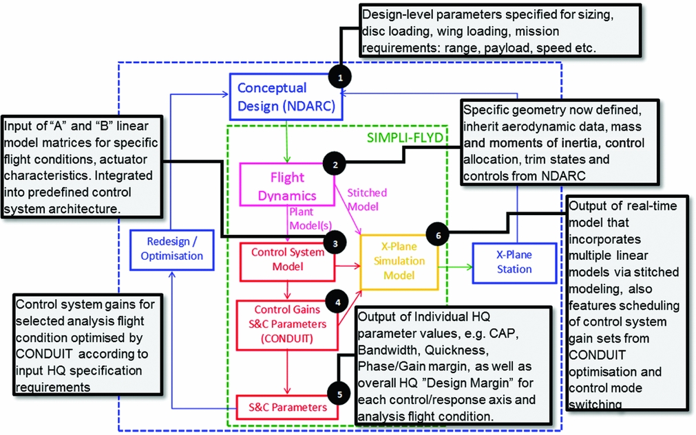
Figure 1 shows the primary components within the SIMPLI-FLYD process and the key interfaces to external components and processes. The dashed blue box indicates the tools and activities encompassed in an overall conceptual design process involving NDARC. The green box is the SIMPLI-FLYD specific functions. Stage (Reference Gorton, Lopez and Theodore1) is the primary conceptual design sizing activity using NDARC. In a future context, this process might be represented by a variety of other analyses encompassed in a MDAO environment. Stage (Reference Gorton, Lopez and Theodore1) is the source of input for SIMPLI-FLYD that encompasses stages (Reference Morris, Sultan, Allison, Schetz and Kapania2) through (Reference Padfield4) where simplified linear flight dynamics models are calculated, integrated with control laws, and then analysed and optimized by CONDUIT. The output of stages (Reference Morris, Sultan, Allison, Schetz and Kapania2) through (Reference Padfield4) are set(s) of stability, control and HQ parameters (stage Reference Andrews5), and an X-Plane compatible real-time simulation model for use in an X-Plane simulation station (stage Reference Johnson6). Reference Lawrence, Berger, Theodore, Tischler, Tobias, Elmore and GallaherReference 7 reports a full description of SIMPLI-FLYD and its sub-functions; some of the key aspects are highlighted in the following section:

Figure 1. SIMPLI-FLYD architecture for including stability and control analysis into conceptual design.
1.1.1 Flight dynamics modelling
The flight dynamics modelling uses a modular approach to represent a vehicle with various combinations of rotors, wings, surfaces and auxiliary propulsion, similar to NDARC. The modelling capability is intended to be configuration-agnostic and the modular framework allows any number of rotors/propellers, wings, tails, and jets. The imported data from NDARC consists of geometric, aerodynamic, and configuration data about the vehicle and pre-calculated trim data for the flight conditions to be assessed. The flight dynamic calculations then loop over the flight conditions calculating linear stability and control derivatives for each rotor, wing, aerodynamic surface and fuselage component separately. For calculation of the rotor contributions, the SIMPLI-FLYD process uses a blade element model which is initialized at the NDARC calculated trim state and uses numerical perturbation to calculate the stability and control derivatives. For the other components, a more simple calculation of the linear derivatives is performed using a mix of analytical and empirical models.
The total vehicle linear models are then computed through the concatenation and summation of the state-space ‘A’ and ‘B’ matrices from the various components. The linear models can be optionally 6-Degree-of-Freedom (6-DoF) rigid body states only, or can include first-order flapping equations, with one longitudinal and one lateral per ‘main’ rotor, akin to the ‘hybrid’ model formulation in Tischler(Reference Tischler and Remple10). As such, a single main rotor configuration linear model has 11 states: 9 rigid body states (u, v, w, p, q, r, φ, θ, ψ) and 2 rotor states (β1c 1, β1s 1) as the tail rotor derivatives are always reduced to their 6-DoF contribution (no flapping terms in linear model). Other configurations that feature two main rotors, for example, such as a tiltrotor or a tandem, would contain 13 states, with 4 rotor states (if included).
For the control derivatives, a simplification was imposed for the CONDUIT point analysis flight dynamic models such that any vehicle always has a fixed set of four ‘controls’ for the primary roll, pitch, thrust and yaw response axes. The effects of multiple or redundant control effectors such as combinations of rotor controls and wing or aerodynamic surface controls are combined via an NDARC-defined ‘mixing matrix’ in advance of analysis at stages (Reference Raymer3) and (Reference Padfield4) (the separate control derivatives are retained for use in the real-time model). The actuator characteristics are configurable for each analysis point model to allow representation of different actuator classes (i.e. swashplate vs aerodynamic surfaces) required for particular flight conditions/configurations. The models can have secondary controls (on rotors, aerodynamic surfaces or auxiliary propulsion) that can be configured to be pilot operated but those are open-loop and used only for real-time simulation.
1.1.2 Control system modelling, analysis and optimisation
The control system applied to the vehicle model at stage 3 (Fig. 1) is based on an explicit model-following architecture that consists of independent feed-forward and feedback paths as shown in Fig. 2. The control laws use a generic architecture with varying modes appropriate for use at different flight conditions as per Table 1. The response types selected are well established for rotorcraft and also are suited to application across a range of vehicle configurations and flight conditions. More augmented response types such as Attitude Command Attitude Hold (ACAH) and Translational Rate Command (TRC) are potential future developments offering a more specific control system design element to the conceptual design analysis. The addition of these response types is possible in the SIMPLI-FLYD/CONDUIT framework but would require new developments and not easily directly implementable by a user. The current response types offer a practical start point for this new tool and meet the initial requirements of a representative control system that can be applied generically to a range of vehicle configurations and enable a more representative analysis of the flight dynamics and control characteristics of a design than a bare-airframe analysis permits.
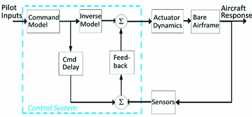
Figure 2. Explicit model-following architecture.
Table 1 Control system response types for various axis and flight modes
RCAH = Rate-Command/Attitude-Hold.
RCDH = Rate-Command/Direction-Hold.
RCHH = Rate-Command/Height-Hold.
The configuration and optimisation of the control laws is fully automated within CONDUIT and the overall SIMPLI-FLYD process (based on certain user configurations). The control system is optimised for each axis where key metrics are used to assess the level of over-or under-design in the control system, for both the feedback and the feed-forward paths. In the case of feedback, the metrics are for the control system (combined with the vehicle) stabilising performance robustness and ability to reject disturbances. Starting with a baseline required value for each specification (defining 0% over-design), the requirements are progressively increased (more over-design) until a feasible design can no longer be achieved. If the baseline design cannot be met, the requirements are decreased (under-design) until a feasible solution is achieved. After the feedback path is optimised, the feed-forward path is optimised using specifications such as piloted attitude bandwidth, attitude quickness, and control power. The optimisation is carried out in a phased process; CONDUIT tunes the gains to first meet all of the ‘Hard Constraints’ (stability specifications), then the soft constraints (the HQ specifications) are optimised. Finally, CONDUIT tunes the gains to reduce the Summed Objective (‘cost of feedback’ or performance specifications) to find the design that meets the requirements with the minimum cost (e.g. such as actuator requirements).
The HQ specifications used to drive the control system optimisation are divided by aircraft type, flight regime, control axis, and feedback or feed-forward. Specification boundaries are drawn from the rotorcraft specifications in ADS-33E(11) and the fixed-wing specifications of MIL-STD-1797B(12). For the full list of the specifications currently used in SIMPLI-FLYD, see Reference Lawrence, Berger, Theodore, Tischler, Tobias, Elmore and GallaherRef. 7. A relatively straightforward user-configurable spreadsheet is used to select the specifications from the CONDUIT library, it is possible for advanced users to add new specifications to the CONDUIT library which could then be linked to the SIMPLI-FLYD analysis.
Once the control system optimisation is complete, the block diagram parameters (feedback gains, feed-forward gains, inverse model parameters, etc.) and the HQ specification results of the control system optimisation, given individually for each axis, are saved for output and further use.
For each individual handling quality specification parameter, a percent over/under margin value is also calculated: this is the % relative value achieved versus the desired minimum specification value as illustrated in Fig. 3 for a typical bandwidth calculation. As shown in Fig. 3, 100% Design Margin (DM) is the value of a specification to transition from 0% over-design, which is on the boundary between Level 1/2 to the boundary of Level 2/3 (−100%) – achieving performance greater than the desired specification, as demonstrated in Fig. 3, is a positive DM or over-design.
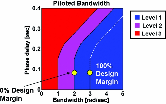
Figure 3. Percent over-/under-design measured based on ability of aircraft to meet/exceed each performance metric.
The CONDUIT analysis then provides a single HQ requirements DM for both the feedback and feed-forward control paths of each of the primary control axes analysed (roll, pitch, yaw, vertical). The assigned axes feedback and feed-forward DMs are the percent over/under design for the worst or limiting specification for each feedback/forward/axis combination. For example, if for ten different roll axis feedback HQ specification parameters, nine achieved a +60% over design but one achieved only 0%, then the roll feedback axis would be assigned a 0% DM.
1.1.3 X-Plane real-time simulation
The other key output feature of the SIMPLI-FLYD toolset is the capability to generate a piloted real-time simulation of the vehicle conceptual design. The X-Plane simulation capability is intended to augment the overall conceptual design process by offering an opportunity to get a ‘sense’ of how different flight dynamics and control characteristics of the conceptual designs manifest themselves when flown pilot-in-the-loop. The piloted simulation is not intended for rigourous HQ analyses but it provides an environment where the flight dynamic characteristics can play a part in examining design trade-offs when flown in representative operational scenarios.
The real-time simulation is based on a MATLAB/Simulink based ‘stitched model’ flight dynamics mathematical model. A stitched model (Reference Forrester, Sóbester and KeaneRefs 13 and Reference Duda14 are examples used and developed by the authors previously) is a method by which multiple linear state-space models are “stitched” together via their constituent trim states and stability and control derivatives being look-up table functions of flight condition and configuration. This type of model offers the ability to represent changing trim and dynamic characteristics across the flight envelope in a model architecture that has a more direct correlation with the linear point condition models. The approach also has added advantages in that it avoids some of the overheads in complexity, robustness and computational demand that more sophisticated non-linear real-time models require – an important consideration in the context of rapidly evaluating lower complexity models of wide variety of configurations in a conceptual design methodology.
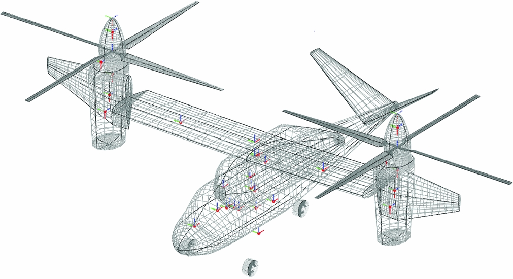
The real-time stitched model is integrated with additional modelling for undercarriage, powerplant and actuators and combined with a control system model that features gain scheduled versions of the control laws optimised at the CONDUIT analysis stage. The anchor points for the gain scheduling are specified by the user and are the result of CONDUIT optimisations at point models through the desired envelope. The real-time control system also has a number of features to enable gross manoeuvring (loops, rolls, etc.), protection against integrator wind up as well as mode switching, blending and logic for transition between weight-on-wheels, hover/low-speed, and forward flight modes. The simulation runs in real time from the MATLAB/Simulink GUI console and communicates data to/from the X-Plane simulation environment using a shared memory interface developed with the support of Continuum Dynamics Inc. and a number of NASA Ames Research Center Aeromechanics office interns. X-Plane provides the interface to the pilot inceptor hardware and provides the graphical scene as depicted in Fig. 4. It can be run on a desktop computer with off-the-shelf gaming pilot control sticks or a more immersive pilot station with multiple displays. Recently, some successful early experimentation has been carried out using an Oculus Rift Virtual Reality Headset instead of computer monitors to provide the visual scene.

Figure 4. Typical X-Plane graphics of some SIMPLI-FLYD models and fixed-based simulator station.
2.0 NDARC/SIMPLI-FLYD COUPLING – MOTIVATION AND METHODS
In this paper, the results of two different analyses will be presented, (1) the coupling of the full NDARC and SIMPLI-FLYD analyses and (2) a study of the sensitivity of the stability and control derivatives calculated by SIMPLI-FLYD to the parameters it imports from NDARC. Referring to Fig. 1, these analyses exercise and demonstrate the modelling and analysis capabilities of the tool stages 1 through 5 and the subsequent feedback path to the core conceptual design/sizing activity represented by the NDARC tool. The X-plane simulation capability (stage 6), although introduced as a capability of the toolset, is not within the scope of this paper.
In this section, the motivation for carrying out each of the analyses and the methods applied are first presented: The primary objective was to develop and assess NDARC and SIMPLI-FLYD coupled in a combined analysis. The goal of the NDARC/SIMPLI-FLYD coupled analysis was to run sweeps of illustrative input parameter variations relevant to the HQ of the design scenarios selected (pitch axis forward flight or yaw axis hover HQs) and examine the impact on both the SIMPLI-FLYD HQ output and the NDARC design sizing. The intent of this analysis is not to present specific handling quality relationships with conceptual design variables such as disc loading or wing loading but to demonstrate the sensitivity of the analysis to the more fundamental input parameters that the HQ analysis would receive from the main conceptual design/sizing processes. The conceptual design process can, for example, arrive at the same disc loading or wing loading from a near-infinite combination of vehicle parameters and configurations; thus, at this stage, the objective is to provide data to enable consideration of the methodology used, and gain insight to what is important/significant for the conceptual design process.
The main task for the preparation of the NDARC/SIMPLI-FLYD coupled analysis was the creation of Python-based ‘wrapper’ scripts which handled the input data and variable initialisation, called the NDARC and SIMPLI-FLYD (via Matlab) codes, and handled the data interface and collection in a common environment. The NDARC run and utility functions were drawn from the ‘rcotools’ library, a Python-based toolset being developed by NASA for the integration of NDARC into the OpenMDAO environment.
The derivative sensitivity study and the NDARC/SIMPLI-FLYD coupled process used the same two NDARC models as input. The models were of a tiltrotor aircraft similar in size and design to an XV-15, with the focus being the pitch axis in forward flight, and a single-main rotor helicopter similar in size and weight to a UH-60A, with a focus on the hover yaw axis characteristics.
3.0 RESULTS
3.1 Stability and control derivative sensitivity analysis results
The results of the sensitivity analysis of the bare-airframe stability and control derivatives to a subset of the input parameters imported by SIMPLI-FLYD are presented first. At this stage, this analysis is not a built-in feature of SIMPLI-FLYD but is facilitated by using a number of the primary sub-functions. Because of its research analysis focus, a number of its configuration parameters are hard-coded for the specific example cases but, as will be discussed later in the paper, the methodology applied could form the basis of a future capability.
The results using the NDARC XV-15-like tiltrotor as the source of input to SIMPLI-FLYD are shown in Fig. 5. Each sub-plot is a 3-axis bar chart. The vertical axis is for the stability and control derivatives being examined, the pitch moment (M), and vertical force (Z), derivatives with respect to control inputs (elevator and rotor longitudinal cyclic) and key longitudinal axis states: pitch rate (q) and vertical velocity (w). The derivative naming convention is the force/moment separated by an underscore from the state/control, e.g. M_elevator or Z_w. The second axis is for the input parameters of the particular component being perturbed (each plot is for a single component) and only the input parameters having a non-zero effect are shown.

Figure 5. Sensitivity of component pitch stability and control derivatives to input parameters imported from NDARC model (tiltrotor, aircraft mode, 200 Kn).
The third axis is the value of the stability and control derivative ‘sensitivity’ which is in fact the derivative of the stability or control derivative with respect to the perturbed input parameter. These sensitivity derivatives have been scaled (to fairly compare different types of derivatives) and the variable perturbations Pj have been ‘weighted’ to allow equal comparison of the component input parameter contribution effect on the overall vehicle. The premise of the combination of the weighting and perturbation size is firstly to perturb each input variable by approximately proportionate size, percentages would be ideal but many variables have a zero value and therefore computing an initial value percentage perturbation is impossible, so a perturbation value reflecting a ‘plausible’ range was selected. For example, perturbing rotor radius and chord by the same dimensional amount would be inappropriate as the value would represent a significantly larger proportion of its starting value or its ‘plausible’ range. The plausible range is important for values which are initially zero in a design, for example delta-3 angle. Here, a perturbation size must be selected to compute a sensitivity without causing inappropriately large (or small) variations in the input parameter for the calculation in the models.
 $$\begin{equation*}
\frac{{\partial \left( {\frac{{\partial {X_i}}}{{\partial {x_k}}}} \right)}}{{\partial {P_j}}} = \left| {\frac{{{{\frac{{\partial {X_i}}}{{\partial {x_k}}}}_{\left( { - {P_j}} \right)}} - {{\frac{{\partial {X_i}}}{{\partial {x_k}}}}_{\left( { + {P_j}} \right)}}}}{{2{P_j}}}\tau \ } \right|,\ {P_j} = {W_j}{{\rm{\Delta }}_j}
\end{equation*}$$
$$\begin{equation*}
\frac{{\partial \left( {\frac{{\partial {X_i}}}{{\partial {x_k}}}} \right)}}{{\partial {P_j}}} = \left| {\frac{{{{\frac{{\partial {X_i}}}{{\partial {x_k}}}}_{\left( { - {P_j}} \right)}} - {{\frac{{\partial {X_i}}}{{\partial {x_k}}}}_{\left( { + {P_j}} \right)}}}}{{2{P_j}}}\tau \ } \right|,\ {P_j} = {W_j}{{\rm{\Delta }}_j}
\end{equation*}$$
The scaling parameter is τ. These allow the numerical sensitivity of the different derivatives  $( {\frac{{\partial {X_i}}}{{\partial {x_k}}}} )\ $to be compared fairly; for example, the M_u derivative may have typical values of approximately of the order of 10–2 whereas M_q is more likely of the order of 100, again calculating a percentage may not be possible because the initial values maybe zero or very small.
 $$\begin{equation*}
{\tau _1} = \frac{{{M_a}}}{{\rho {V_{{\rm{ref}}}}{A_{{\rm{ref}}}}}},\ {\tau _2} = {l_{{\rm{ref}}}},\ {\tau _3} = \frac{1}{{{V_{{\rm{ref}}}}}},
\end{equation*}$$
$$\begin{equation*}
{\tau _1} = \frac{{{M_a}}}{{\rho {V_{{\rm{ref}}}}{A_{{\rm{ref}}}}}},\ {\tau _2} = {l_{{\rm{ref}}}},\ {\tau _3} = \frac{1}{{{V_{{\rm{ref}}}}}},
\end{equation*}$$
where τ is a function of combinations of τ1, τ2 and τ3 according to the units of the derivative as per Table 2.
Table 2 Scaling parameters for sensitivities of various stability derivatives

The colour in these plots does not represent any value and is merely intended to help to differentiate between each row of the plot data. For reasons of clarity, only the key derivatives known to influence those dynamics relevant to the pitch or yaw axis HQ DMs for the two example cases are presented.
The main premise of the analysis is to focus on the relative values (sensitivity) rather than the absolute values computed. The figures show the sensitivities for one of the rotors (both rotor results are identical in this forward flight condition), the wing, the fuselage, the horizontal tail, and one of the two ‘end plates’ of the H-tail configuration (same result for both). The sensitivity axes scale is equal across the plots to allow direct comparison. Comparing across all the plots for the different components, it is immediately clear that the majority of the rotor parameters have a weak influence on the longitudinal stability control derivatives in aircraft mode of the tiltrotor. The greatest sensitivity observed for the rotor parameters is the radius and X position (longitudinal) on the M_q (damping in pitch) and M_w (angle-of-attack stability) derivatives. Intuitively, the input parameters that influence the pitch derivatives the most, and are at least an order of magnitude more ‘sensitive’ than the rotor parameters, are the horizontal tail parameters such as the tail area, X position, lift curve slope (C L α), elevator control area and control flap lift effectiveness (C L δf). The only other parameter presented that approaches the same level of sensitivity to the horizontal tail input parameters is the wing X-location influence on the M_w derivative.
Figure 6 shows the same analysis for the single-main rotor helicopter configuration at hover for a number of the key lateral-directional axis bare-airframe stability and control derivatives that would influence the yaw axis HQ. At hover, the derivatives are most sensitive to the input parameters defining the tail rotor, though the main rotor equivalent hinge offset approaches a similar order of sensitivity. The most sensitive parameter of the tail rotor is the radius, followed by the tail rotor X position and blade chord (chord). The results are mostly intuitive although the inclusion of some of the lateral-directional coupling derivatives show relationships that are less intuitive, such as the effect of the tail rotor radius and Lock number on the overall vehicle roll-due-to-yaw derivative, Lr.

Figure 6. Sensitivity of component lateral-directional stability and control derivatives to input parameters imported from NDARC model (single-main rotor configuration, hover).
3.2 NDARC/SIMPLI-FLYD coupled analysis results
The results of applying variations to input parameters in the full coupled NDARC/SIMPLI-FLYD analysis are presented in the following section. The sensitivity analysis of the previous section guided the selection of a subset of design variables to use. The same two NDARC models, an XV-15-like tiltrotor, and a single main rotor helicopter (similar to UH-60a) were used as the test example vehicles. These results build upon the work in Reference Lawrence, Berger, Theodore, Tischler, Tobias, Elmore and GallaherRef. 7 in two aspects: (1) for each change of variables, NDARC now performs a sizing task (the previous analysis varied the design which affected the weight but did not re-size), and (2), the analyses use multidimensional changes to input variables rather than single parameter sweeps and thus are able to demonstrate coupling effects of input parameters on the HQs.
The NDARC sizing task determines the dimensions, power, and weight of a rotorcraft that can perform a nominal design mission(Reference Johnson8). The aircraft size is characterized by parameters such as design gross weight, empty weight, rotor disc loading and engine power available. NDARC calculates the size and weight of certain specified aircraft components while factoring in the weight of other components with a predetermined size (such as the parameters being varied in this analysis). The exceptions to this currently are the actuator parameters which are uncoupled to NDARC and only currently affect the HQ and not the design weight and power. In this paper, the changes of the moments of the inertia of the vehicle with respect to the design variations were not directly modelled. Instead, inertia changes are currently represented via the weight change and the use of fixed radii of gyration which SIMPLI-FLYD inherits from NDARC. After NDARC has completed its task, the aircraft design data is input to SIMPLI-FLYD. The final outputs of the SIMPLI-FLYD analysis are the HQ DMs, as calculated by CONDUIT. The CONDUIT HQ DMs were carried forward as the overall HQ analysis metrics for two reasons:
1. The DMs offered a mechanism by which multiple feedback and feed-forward HQ specifications are reduced to two HQ DMs per axis – these, respectively, represent the aircraft's overall flight dynamic stabilization/disturbance rejection and control response characteristics for each axis.
2. The DMs are a non-dimensional metric (% over/under design) based on the worst case HQ specification.
Using this form of DM avoided a situation where each analysis case presented a large array of multiple specifications with differing units and meanings. Instead, the DMs present more holistic metrics of the HQ “goodness” that are more convenient for integration with an overall MDAO process and for presentation to the design engineer.
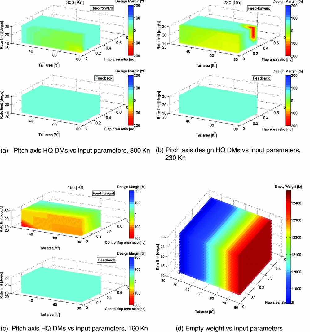
Figure 8(a) to (c) shows the tiltrotor pitch axis HQ DM for a sweep of three input parameters: horizontal tail area, tail flap control area ratio and tail flap actuator rate-limit. Three flight conditions – 300Kn, 230Kn and 160Kn – are evaluated for aircraft mode. All the values varied for the input parameters are listed in the following bullets (*initial nominal value):
• Horizontal tail area: 25.125, 40.2, 50.25*, 60.3, 75.375 (ft2)
• Horizontal tail flap ratio: 0.0647, 0.1656, 0.2587*, 0.36, 0.45 (nd)
• Horizontal tail flap actuator rate limit: 10, 20*, 30 (deg/s)
As described earlier, the analysis computes a DM for both the feedback (stabilisation) and feed-forward (response) components of the pitch axis HQs. The figures use 3D Matlab ‘slice’ plots that provide a colour weighted ‘cloud’ of data for the three input parameters. The colour indicates the DM value, ranging from red for −200% under-DM, to deep blue for the +200% over-DM. The plots are a space-efficient method for presenting up to 3/4-dimensions of data. The printed versions are somewhat limited in that the slices can only be viewed from a fixed perspective; whereas, in the Matlab software, the user can manipulate the viewing angle to inspect the data from any vantage. Nevertheless, the main intention is to present the broader trends, which, in these cases, are sufficiently displayed by this compact form of data presentation.
The first result to highlight is the trend with flight speed, where the sensitivity of the DMs to variations in the input parameters reduces with greater airspeed. Here, the higher dynamic pressure confers increased bare-airframe stability, damping and control power, improving the ability of the aircraft to meet the stabilisation (feedback) and control response (feed-forward) HQ specifications, respectively. As the speed reduces, and particularly at 160Kn (which is approximately 1.5x the stall speed in aircraft mode), the boundaries between over-design and under-design in the pitch HQs become more apparent. Intuitively, the worst pitch axis feed-forward HQs (under design) are for the smallest tail, flap and lowest actuator rate limit. Note that throughout these analyses, to save computational time by preventing the CONDUIT optimisation continuing to very high positive DMs, a limit was applied that prevented further optimisation if a +60% DM was reached.
Figure 8(a) shows that another region of reduced DM emerges, indicating that the tail can be ‘too big’ from an HQ perspective. In these cases, the large tail with small control surface, at low rate limit, has under-design for the feed-forward pitch HQs. The aircraft is over-damped and/or too stable whilst the control power is reduced by the smaller control surface, and thus, the aircraft is unable to meet certain control response specifications. Examination of the detailed output (not shown) revealed that the limiting specifications that were sub-Level 1 were the control power (normal force (Nz) in pull up), and the Control Anticipation Parameter (CAP), which is also strongly affected by the ability to command Nz. This confirms that lack of control power that is a limiting factor, however it is observed that for smaller tail areas with the same smallest flap ratio, the DM is not sub-Level 1 (the yellow/green areas). This demonstrates the control response vs stability trade-offs of tail and control surface size.
In the tiltrotor examples, varying the tail flap actuator rate limit had different effects on the outcome of the feed-forward and feedback DMs. For the feed-forward DMs, the rate limit had a graduated effect where the increased rate limit was able to affect the DM achievable for varying tail area and flap area ratios. The feed-forward specifications have a number of time-domain specifications which are sensitive to non-linearity such as rate-limiting. Conversely, the overall feedback DMs had no sensitivity to rate limiting (for the parameter range examined), probably because the feedback specifications are predominately linear system analyses and the non-linear effect of rate-limiting essentially plays no part in determining the margin to these specifications. The exception is the Open Loop Onset Point (OLOP) specification(Reference Duda14) which is included in both the feed-forward and feedback analysis to capture the effect of rate-limiting. OLOP was primarily developed to predict HQ issues due to pilot input induced rate limiting and there are clear guidelines to evaluate the OLOP specification using the maximum pilot input (i.e. full stick throw). However, the use of OLOP as a feedback HQ specification in SIMPLI-FLYD is an extrapolation of its original design. As such, the concept of the pilot input is no longer applicable, and instead, an external disturbance (gust, etc.) is used. A ‘maximum’ disturbance value is required, for which a nominal value of 5 ft/s in the vertical velocity (w) was selected. However, closer inspection of the feedback optimisation discovered that the OLOP specification was not a limiting factor for any of the cases examined. The OLOP parameter for the cases that would be expected to be the ‘worst’ from this perspective, i.e. those with smallest tail and control flaps, are shown for a range of actuator rate limits in Fig. 7. OLOP limits are not approached even for the smallest tails which should require the greatest feedback stabilisation due to the reduction in bare-airframe stability. Hence OLOP, the only feedback specification that would be sensitive to actuator rate limiting, does not act as a limiting specification and no relationship is observed with rate limit for the overall feedback DM.
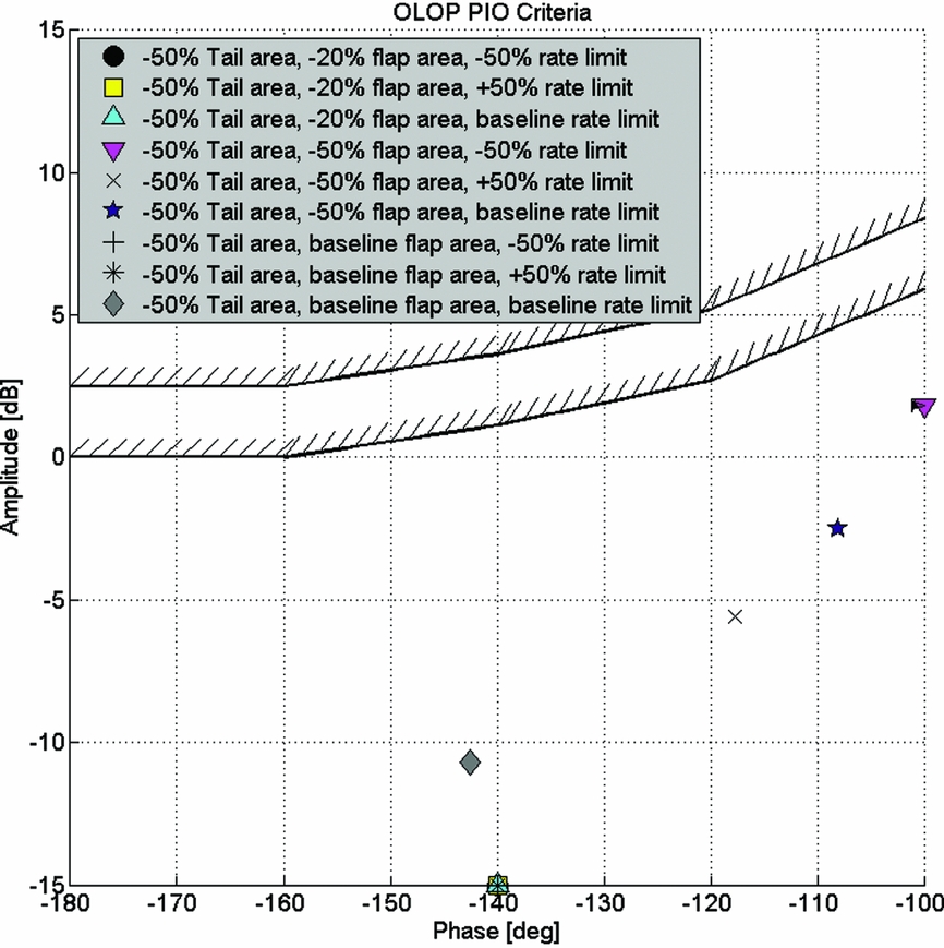
Figure 7. Variation in OLOP specification at 50% reduced tail area for range of control flap areas and control flap rate actuator rate limits.
The relationship of the empty weight with respect to the three design variables is shown in Fig. 8(d). The tail area is the dominant factor affecting the aircraft weight. The tail flap area ratio has a relatively weak effect. The actuator characteristics have no effect as NDARC does not know anything about those. Currently, the actuator properties are only an input to SIMPLI-FLYD and thus can only influence the HQ DMs. The “cost” of changing the actuator performance on the design, such as in terms of weight, is not yet modelled and is a planned future development.

Figure 8. Tiltrotor feed-forward/feedback pitch axis HQ DMs and empty weight for variations in tail area, tail flap area ratio and tail flap actuator rate limit at various speeds (aircraft mode, sea level).
Figure 9 is a comparative set of sweeps for the tiltrotor at the 160Kn aircraft condition. In these cases, however, the actuator rate limit is fixed at the nominal 20deg/s, and the third axis (vertical) of input parameter variation is now the horizontal tail longitudinal position, expressed in non-dimensional terms, X/L (X-location divided by the reference length of rotor radius), for values of 1.4317, 1.7896*, 2.1475 (*nominal). Sensitivity of the DMs (a) is observed for all three variables. Vehicle empty weight (b) is mostly affected by the tail area and X-location. Comparing the feedback and feed-forward DMs, a trade-off is seen between an optimal configuration for stability (feedback) and response (feed-forward). The feed-forward tends to prefer a larger control surface on a smaller tail for the intermediate tail location and the feedback prefers a larger tail, at the largest X-location and is only weakly sensitive to the flap size (the very smallest tail is improved by having a bigger fraction of control surface).
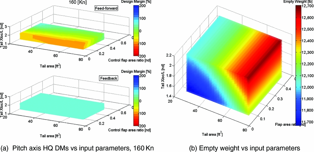
Figure 9. Tiltrotor feed-forward/feedback pitch axis HQ DMs and empty weight for variations in tail area, tail flap area ratio and tail non-dimensional longitudinal position (X/L), at 160Kn (aircraft mode, sea level).
The results of the NDARC/SIMPLI-FLYD coupling applied to the single main rotor helicopter, with the focus on the yaw axis HQ are shown in Fig. 10. The DMs are shown for a sweep of the tail rotor size (a coupled increment in rotor radius at constant solidity and tip speed), non-dimensional longitudinal tail rotor location (X/L) and tail rotor actuator bandwidth. The range of parameters was chosen to investigate whether an optimum size/position existed for rotors smaller than the nominal 6ft radius. Hence, the rotor size variations ranged from 6ft to 3.6ft radius (a 40% reduction) and a longitudinal position, X/L, from 1.3 to 1.82 (a 50% increase from nominal). Note that there is a region of the plot for radii below 5ft and the smallest X-locations that is empty. Here, NDARC was unable to converge on a sizing or trim solution, and thus, these cases were discarded as invalid.
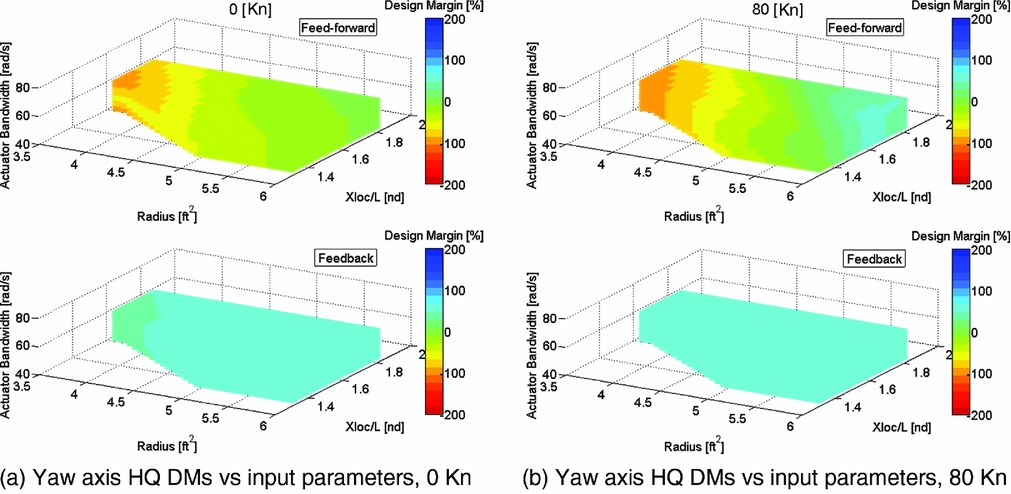
Figure 10. Single main rotor helicopter feed-forward/feedback yaw axis HQ DMs vs tail rotor radius, tail rotor non-dimensional longitudinal position (X/L) and tail rotor collective actuator bandwidth at various speeds (sea level).
For the feedback DM, there is very little sensitivity to the input parameter variations, and almost all cases reached the upper limit of +60% DM. The feed-forward margins exhibited much greater sensitivity to the input parameter variations. The DM improved with increased radius and X-location but only reached a +10% over-DM case with largest rotor, longest tail rotor location and greatest actuator bandwidth value. The DMs at forward speed are shown in Fig. 10(b). Essentially, the same trends as hover are reflected, but the region of positive DM is enlarged. This can be partly attributed to a different performance of the vehicle in this flight condition (such as the empennage becoming effective in forward flight) but also due to different HQ specification requirements being applied for this forward flight condition, which also has a secondary effect in that the CONDUIT control system gains are optimised differently. The DM concept is useful here, as many HQ specifications are not common between hover and forward flight, and the margins provide a constant metric of HQ performance across the changing requirements.
The outcome of only achieving a positive DM in a small portion of the parameter space led to a second sweep for the single main rotor configuration; the results are shown in Fig. 11. The plots show the yaw-axis DMs but for a slightly different set of input parameter variations. The variation in the tail rotor size is retained, but this time, larger tail rotors are examined. However, to ensure design geometry ‘consistency’, instead of specifying the location of the tail rotor directly, a tail rotor clearance (modifying its longitudinal position with respect to the main rotor) was varied. Specifying the clearance was necessary to ensure that the larger tail rotors did not intersect the main rotor disk – and was a more convenient and efficient method than manually recalculating the rotor positions, especially when the NDARC sizing automatically configures the main rotor disk size. Finally, and simply for comparative purposes, instead of actuator bandwidth, the tail rotor actuator rate limit was varied.
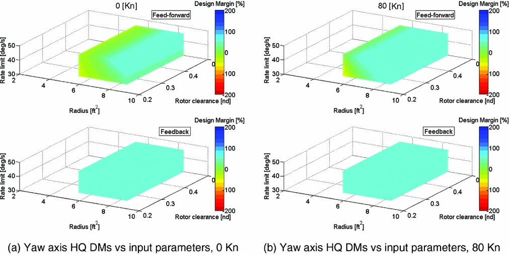
Figure 11. Single main rotor helicopter feed-forward/feedback yaw axis HQ DMs vs tail rotor radius, tail rotor non-dimensional longitudinal clearance and tail rotor collective actuator rate limit at various speeds (sea level).
At hover in Fig. 11(a), a larger region of cases now equal or exceed the 0% DM in feed-forward (feedback is at the +60% limit in all cases). Actuator rate limiting is an influential factor, with its increase enabling a greater proportion of the rotor size/clearance cases to meet the 0% or better yaw axis DM. The change to the forward flight speed condition (b) again enlarges the region of cases with positive DMs.
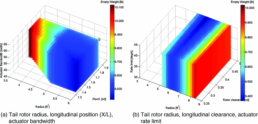
The empty weight for the two sweeps for the single main rotor configuration is compared in Fig. 12. Figure 12(a) shows that for the tail rotor size reduction, the vehicle empty weight actually increases. The reduced size tail rotors are increasingly inefficient and require greater power, which increases weight for a number of the other components of the vehicle. In the second set of sweep cases in Fig. 12(b), a minimum weight region is observed between the smallest and largest tail rotors and towards the larger tail rotor clearance positions.

Figure 12. Single main rotor helicopter empty weights vs input parameters for two different parameter sweeps.
4.0 DISCUSSION OF LESSONS LEARNED AND FUTURE DEVELOPMENTS
As stated earlier, the intention of this paper is not to focus on specific analysis results or design trends but use to the application of the SIMPLI-FLYD tools to well-known configurations to demonstrate the capability but also to provide a framework to discuss the methodology employed and lessons learned so far. This section provides a commentary on the tool, how it has been used, the issues that arose and how they inform how it may be used in future processes.
4.1 Validity of SIMPLI-FLYD for conceptual design processes
The current paradigm for the use of SIMPLI-FLYD in an overall vehicle conceptual design process is that the computed HQ DMs would set the constraints for an optimisation, i.e. some minimum HQ performance is required, 0% or perhaps a positive margin while other design objectives are maximised or minimised, such as the empty weight or flyaway cost. What has been demonstrated so far, is a first ‘cut’: defining appropriate DM levels more conclusively for conceptual design will require the analysis of SIMPLI-FLYD in an analysis combined with many more multidisciplinary design constraints. Additionally, an assessment of the choices of HQ constraints made in SIMPLI-FLYD will require retrospective analysis from later in the design lifecycle – i.e. using higher fidelity tools, models and data available from detailed design to analyse the assumptions and constraints made in the conceptual design phase. Ultimately, the question of how to validate and verify the approach is outstanding – possible approaches could be a more in-depth retrospective study of a design with known outcomes or perhaps shadowing processes using current tools and techniques to establish whether different outcomes are achieved.
4.2 Flight conditions selection for HQ analysis
As was shown, the HQ characteristics and subsequent DMs vary across the flight envelope due to both the changing performance of the vehicle and the specifications applied. For the tiltrotor, using the pitch axis in aircraft mode example, greater criticality emerges mostly at low speed, but not exclusively, with DM degradations occurring at the higher speed for other reasons. This raises questions about how many HQ flight condition analyses should be included. Clearly, if the vehicle can hover and fly at some forward speed, a minimum of two should be assessed, but more could be incorporated. NDARC's sizing typically uses 3–5 critical flight conditions and a similar approach could be taken for the HQ analysis with the approach of some baseline characteristics at a set of nominal flight conditions being analysed. Alternatively, an approach that brackets the operational envelope with min/max airspeed, min/max altitude plus certain configuration changes (e.g. rotor tilt) might be required or considered prudent. The results thus far tend towards a recommendation for the latter, though the level of effort required/appropriate for HQ in conceptual design must be considered.
4.3 Computational speed of HQ analysis
Currently, there is no requirement for how much computational time should be allowed for the HQ analysis in conceptual design; however, if the objective is to explore very large parameter spaces rapidly, the 15–20 minute per flight condition of a NDARC/SIMPLI-FLYD coupled analysis run (all axes) currently required typically on a desktop PC (high-end laptop – Intel Core i7-3280 QM @ 2.7 Ghz, 16 MB RAM) is likely a limiting factor. For comparison, using NDARC as a benchmark for a conceptual design-level tool, usually completes its sizing task in seconds and much less than a minute.
Possible solutions might be a faster running version of SIMPLI-FLYD by streamlining its tasks or incorporating an analogous but alternative approach to the full CONDUIT optimisation. Alternatively, a framework that incorporates the HQ analysis in the design process in a less tightly-coupled approach might allow for the current computational times. In preparing the NDARC/SIMPLI-FLYD coupled analysis runs, it was necessary to down-select a subset of the many possible input variables available to a few of significance for presentation in the paper. In a wider context, the down-selection of input parameters is necessary to reduce the computational task and avoid the “Curse of Dimensionality”(Reference Forrester, Sóbester and Keane13), where for k-dimensions (parameters), nk runs or calculations are required for a full factorial sweep of all possibilities. This is especially relevant when exploring new designs or issues where there is no heuristic knowledge of which parameters may be important to examine or include in an optimisation. Although for the scenarios examined in this paper an experienced flight dynamics engineer could likely choose the most relevant input variables, a method to verify the down-selection process more formally was desirable. This led to the development of the SIMPLI-FLYD stability and control derivative sensitivity analysis presented earlier. The input parameters that most influenced the key stability and control derivatives known to influence the HQ scenarios selected were then selected for investigation in the full NDARC/SIMPLI-FLYD analyses.
During the development of stability derivative sensitivity analysis, it became apparent that the process of importing the NDARC parameters to SIMPLI-FLYD for the calculation of the stability and control derivatives is one of a series of steps in a process of translation and reduction of parameters, as outlined in Fig. 13. At the beginning is an aircraft design in NDARC, defined by hundreds, if not thousands, of parameters defining the geometry, aerodynamics, weights and power. Of these parameters, on the order of 150–250 are imported by SIMPLI-FLYD to define the flight dynamics models with a few additional parameters to define the control actuator characteristics. The flight dynamics (if restricted to rigid-body, 6-DoF) are essentially described by 36 stability derivatives and a minimum of 24 control derivatives. These, in conjunction with the optimised control system gain parameters, determine the approximately 10–20 HQ (feedback and feed-forward) specifications per axis. The most limiting specifications then determine the overall HQ DMs which number up to eight, two parameters per axis, for feedback and feed-forward. Examining the steps of the overall NDARC/SIMPLI-FLYD coupled process, it appears there might be utility in studying the sensitivity between the parameters of each of the constituent steps. Such an approach would allow a piece-wise ‘chain of sensitivity’ to be identified instead of treating the whole process as a ‘black box’. For example, a user may trace the sensitivity of a subset of specifications to a subset of derivatives which in turn are only sensitive to a particular subset of input parameters.
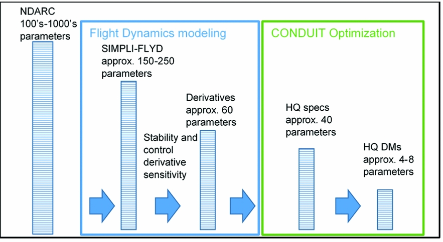
Figure 13. Schematic showing the reduction of the number of parameters from NDARC model to SIMPLI-FLYD handling qualities Design Margins.

Figure 14. An example of OpenVSP geometry with component mass centres identified.
Thus far, the only NDARC/SIMPLI-FLYD sub-stage sensitivity study that has been carried out is the sensitivity of the stability and control derivatives to the SIMPLI-FLYD input parameters. The method offers useful insight into which input parameters are the most important to determining the key stability derivatives for the HQ. Admittedly, in the cases examined, the aircraft designs are well understood (a main wing-aft tail ‘aircraft’ and single main rotor/tail rotor configuration), so any experienced flight dynamics engineer could predict the majority of the outcomes of the sensitivity sweeps; but, as already highlighted, the analysis could be a very useful adjunct when such knowledge does not exist.
The stability derivative sensitivity analysis is able to compute the sensitivity of a full set of 60+derivatives to a number of input variables in much less time than the same SIMPLI-FLYD/CONDUIT control system optimisation and DM calculation would take for the same number of input parameter variations (a stability derivative sensitivity analysis of 60 variables takes ~1 hour, whereas, to compute the equivalent sensitivity of the DM to the same number of input parameters would take >40 hours). With reduced complexity and speed there is cost, and a number of limitations of the sensitivity analysis should be highlighted. Firstly, for any sensitivity analysis, the results are likely configuration-specific and therefore the trends may not apply between different design studies; also they include a modelling simplification, as coupling effects between a change in multiple input parameters on the models are neglected as per classical linear theory. Furthermore, the technique does not consider the effect of performing a re-optimisation of the CONDUIT control system gains after a design change. For example, a method could be devised to achieve an approximate overall sensitivity to infer required design changes to achieve a particular HQ outcomes by combining the stability derivative to design parameter sensitivities with a corresponding sensitivity study of the output HQ parameters to the stability derivatives variations. However, such an approach may lead to unforeseen HQ outcomes of design change couplings when they are included in the full process (i.e. the completion of stages 1–5 in Fig. 1).
Nevertheless, the key advantage is that the calculations for the stability and control derivative and the other sub-stage sensitivity analyses would be much faster. In fact, the whole chain of sensitivities would be faster to calculate than the full process and for many more parameters, since CONDUIT re-optimization of the control system, which is the major computational cost to the current process, would not be carried out. If a simplified surrogate analysis could be developed, a framework incorporating frequent calls of the fast, simplified analyses alongside the more computationally expensive “full” CONDUIT optimisation might lead to an overall more computationally efficient approach.
The trade-off between computational resources and the number of analyses and the rigour they contain is obvious. The number of potential variables that could be involved also highlights challenges in how HQ should be managed in an optimisation. A human in the loop would seemingly be overwhelmed by the number of potential variables that could be used to influence the HQ. However, other design constraints may help to reduce the number of variables that the HQ aspects may reasonably be allowed to influence.
4.4 Moments of inertia estimation and management of vehicle geometry
The estimation of the mass moments of inertia of vehicles is a crucial component in predicting the flight dynamics of a vehicle. The current SIMPLI-FLYD method of representing inertia changes via the weight change combined with fixed radii of gyration is only likely to be satisfactory for gross changes in design weight, and as long as the configuration does not vary drastically. It is not likely to have sufficient accuracy for changes in subcomponents of the vehicle, and furthermore, radii of gyration methods rely on the extrapolation of historic data sets for established configurations. A future development that will greatly improve this is the anticipated integration with the NDARC/SIMPLI-FLYD process of the U.S. Army ADD developed Automated Layout with a Python Integrated NDARC Environment (ALPINE) tool(Reference Perry15). ALPINE provides the capability to generate 3D geometries in Open Vehicle Sketch Pad (OpenVSP)(Reference Gloudemans, Davis and Gelhausen16) from NDARC output. From this 3D geometry, ALPINE then enables a calculation of the mass and inertia properties using OpenVSP's mass properties functions which offer improved resolution to arbitrary configuration changes than the current approach.
A related issue that emerged from performing the analyses in this paper was that even for the relatively simple cases considered, such as when moving a tail, or changing its size, ensuring geometry consistency such as making sure the fuselage adjusts to support the tail brings a design geometry management overhead (NDARC has features that addresses some of these aspects but is not comprehensive). Considering future scenarios where many design adjustments are simultaneously occurring, a manual process could be rapidly overwhelmed. Geometry consistency is not only important to ensure that the design is valid structurally (i.e. components are attached), but also for capturing design cross-couplings from a HQ perspective. For example, moving the horizontal tail for better HQ/weight savings may impact the vertical tail location, depending on the configuration, and thus may affect the lateral-directional characteristics. Indeed, a 3D geometry engine approach to managing the design configuration, such as that provided by OpenVSP, would also be advantageous when manipulating a design's geometry (manually or automatically) as well as integrating the aforementioned moment of inertia considerations. This experience in ensuring geometry consistency correlates with the considerations of Reference Johnson and SinsayRef. 17, which states the importance in placing a 3D geometry engine at the heart of any future conceptual design environments.
4.5 The importance of actuator characteristics
Finally, although the emphasis of this paper has mostly been to demonstrate the sensitivity of the HQ to physical parameters of conceptual design, the results in this paper reinforce the conclusions of Reference Lawrence, Berger, Theodore, Tischler, Tobias, Elmore and GallaherRef. 7 that in SIMPLI-FLYD, the actuator characteristics play an almost equally important role in determining the HQ DMs. User selection of the actuator characteristics must be carefully considered. Furthermore, cost models for the actuators in terms of weight, size, power and monetary cost as function of their performance characteristics must be incorporated into this analysis if HQ that are reliant on automatic control are to be validly considered in a conceptual design.
5.0 SUMMARY AND CONCLUSIONS
This paper has reported the exploration of the recently developed SIMPLI-FLYD toolset. The use of Python-based scripting has enabled the integration of NDARC and SIMPLI-FLYD to facilitate learning about how HQ analyses interact with conceptual design model variations. Processes have been demonstrated that can calculate DMs with respect to HQ specification criteria while also evaluating the vehicle design weight and other design metrics. Also, secondary techniques like the bare-airframe stability and control derivative sensitivity analysis offer insight to the inner-workings of a complex, multi-step process. The automation provided by SIMPLI-FLYD already provides significant efficiencies over traditional approaches in enabling a user to progress from sizing a vehicle to stability, control and HQ in a few automated steps without requiring extensive flight dynamics and control modelling knowledge. Nevertheless, if very large design spaces are to be explored, as might be common in some conceptual design processes, the speed of analysis may still be unsuitable. The sensitivity analysis techniques of the key constituent steps of SIMPLI-FLYD, such as the stability and control sensitivity analysis, may offer pathways to mitigate the computational cost of running a ‘full’ CONDUIT optimisation for every design iteration or gradient search if faster run times become a requirement.
The following items are highlighted from using the tools in a coupled approach to examine different vehicle types, varying a mix of input parameters and flight conditions, and evaluating different HQ issues:
• The calculated HQ DMs vary across the flight envelope due to both changing flight dynamics and control characteristics and the HQ requirements specifications applied. Using the CONDUIT percent over/under-DM methodology for the overall HQ analysis reduced the HQ output metrics to a quantity and non-dimensional format that was convenient for assessing the HQs consistently across this range of flight conditions and axes with varying requirements.
• The current SIMPLI-FLYD analysis for a single flight condition is relatively computationally expensive when compared to an NDARC sizing run, around 1–2 orders of magnitude slower for the same number of flight conditions analysed. If rapid exploration of large design spaces is desired, this speed is likely to impose constraints on how to deploy the tool in a future design process and requires further evaluation of what HQ aspects should be incorporated (and how) if similar speed of analysis to NDARC sizing is required.
• It has already been established that HQ analyses of the bare-airframe alone of the majority of rotorcraft designs are insufficient. The required inclusion of a representative control system results in an analysis where the actuator performance characteristics influence the HQ DMs as strongly as aircraft geometric and other ‘physical’ design characteristics. Therefore, their cost (in terms of weight, power requirements, etc.) is critical, and needs to include sufficient sensitivity to variations that are important to HQ to achieve a valid overall design optimisation that includes HQ characteristics dependent on a closed loop flight control system.
ACKNOWLEDGEMENTS
The authors would like to acknowledge Larry Meyn, NASA Ames Research Center, for his support in the development of the Python scripts and the provision of the ‘rcotools’ library. Andrew Gallaher, U.S. Army ADD, Moffett Field is acknowledged for OpenVSP and Python development support. Travis Perry is thanked for the provision of OpenVSP images.