


NOMENCLATURE
- M
mass matrix
- C
damping matrix
- K
stiffness matrix
- F
force vector
- Φ
mode shape matrix
- q
generalised coordinate
- m
mass of the exciter moving coil
- c
damping of the exciter
- k
support stiffness of the exciter
- B
strength of the magnetic field
- L
length of the single-turn coil
- N
number of turns of the coil
- I
current across the exciter coil
- G V
gain of power amplifier
- V’
voltage of the exciter coil
- V
input voltage of the power amplifier
1.0 INTRODUCTION
Flutter is a self-excited oscillation in which the amplitude of the elastic structure is not attenuated by the coupling of unsteady aerodynamic forces, elastic forces and inertial forces(Reference Dowell, Bendiksen, Edwards and Strganac1). It is a very dangerous phenomenon that can lead to catastrophic consequences during flight of high-speed aircraft. With the rapid development of computational structure mechanics and computational dynamics, great progress has been made on numerical flutter prediction methods(Reference Schuster, Liu and Huttsell2). High-quality mathematical models are required for numerical predictions, while some assumptions must always be made to simplify the aircraft structure, aerodynamics and flight control systems. It is difficult to consider all the nonlinear and uncertain modelling errors that may sometimes lead to large deviations from complex real-life engineering applications. Experimental flutter testing is therefore another important method to investigate complex aeroelastic effects.
Flight testing can be applied to confirm the complete aeroelastic behaviour in the actual working environment. However, not only are flight tests very expensive and suffer from great risk, but the measured data are also limited. The most important limitation is that it is impossible to carry out flight testing in the initial design stage without detailed validation and verification using other methods. Therefore, wind-tunnel testing has became a very important method for flutter investigations(Reference Yang, Wang, Zhang and Liu3,Reference Xuan, Han, Zhang, Yun and Chen4) . Wind-tunnel tests can take into account the effects of aerodynamic forces, but the aeroelastic test model must be designed and scaled carefully due to the size of the test section of the wind tunnel. Also, the mechanical characteristics of a scaled aeroelastic model may exhibit obvious differences from the full-scale aircraft structure. Wind-tunnel flutter testing is still very expensive, and also may sometimes be very difficult to implement, for example for aeroservoelastic problems related to large, high-speed aeroelastic models.
Other types of ground flutter test methods without requiring the use of a real wind tunnel are thus also required to simulate the aerodynamic forces. As early as the 1960s, Kearns proposed the concept of ground flutter simulation and made preliminary attempts(Reference Kearns5). Up until the 1980s, Pan and Qi also conducted preliminary research(Reference Pan and Qi6). They tried to simulate the unsteady aerodynamics using an exciter and applied the sensed speed as a feedback signal to predict the flutter. They also tried to conduct thermal flutter tests by heating using a quartz infrared lamp. However, due to the limitations of the test conditions and hardware applied, these two test methods did not apply real-time control of the loading system during their operation. In addition, due to the limitation of the multi-input and multi-output (MIMO) vibration excitation method and the low maturity of fast calculation algorithms, such research attracted little attention from both academia and the industrial community.
In the early years of the twenty-first century, with the rapid development of flutter technology, computer technology and control technology, real-time calculations became possible. At the same time, aeroelastic and aeroservoelastic problems related to high-speed flight vehicles in high-temperature environments also started to attract great attention. In 2001, the Central Aerohydrodynamic Institute (TsAGI) of Russia proposed the electromechanical method (EMM)(Reference Naryzhny, Pedora and Smyslov7), which uses a digital computer to calculate unsteady aerodynamic forces based on structural vibration information measured in real time and considers the unsteady aerodynamic forces on the structures by the exciter. Ground flutter testing without a real wind tunnel is called the DWT approach, which returns to the designer’s original vision and is now attracting increasing attention (Reference Zeng, Kingsbury, Ritz, Chen, Lee and Mignolet8). A DWT system uses the concentrated force of excitation devices to simulate an equivalent unsteady aerodynamic force instead of using a real wind tunnel. The DWT concept proposed by ZONA Company in 2011(Reference Zeng, Kingsbury, Ritz, Chen, Lee and Mignolet8) is very similar to the EMM technology of TsAGI. Closed-loop coupling of the structure and aerodynamics is achieved via real-time measurements of the structural response, real-time calculations of the unsteady aerodynamics and real-time control of the loading applied by the excitation devices. DWT technology has great potential to confirm and validate preliminary designs of flight control systems for high-speed elastic aircraft. Later, Wu et al. carried out theoretical research on unsteady aerodynamic loading simulated using exciters, and carried out pneumatic servoelastic semi-physics simulation tests on a slender-body missile model with a flight control system(Reference Wu, Chu, Yuan, Yang and Tang9,Reference Xu, Wu and Yang10) . Yang and Song et al. designed a H ∞-robust controller for the siding structure and carried out ground aeroelastic simulation testing(Reference Song11). Zhang et al. studied an engineering-oriented modelling procedure and a flutter analysis method for a fin-actuator system in both the frequency and time domains(Reference Zhang, Wu and Yang12). Wu et al. further applied ground flutter aerodynamic simulation technology for flutter analysis of a full-motion rudder with more exciters(Reference Wu, Ma and Yang13).
Although great progress in DWT technology had been made recently, many key issues remain for further investigation; For example, most research to date has only applied classical system identification methods to model ground flutter test systems(Reference Zeng, Kingsbury, Ritz, Chen, Lee and Mignolet8,Reference Song11,Reference Wu, Ma and Yang13) . However, models based on classical system identification algorithms are equivalent models in which the model parameters lack physical meaning. In contrast to traditional model identification methods, the subspace identification method can yield a state-space model for the system in the presence of certain input noise, output noise and state noise, achieving good performance(Reference Song, Yang and Wang14-Reference Li, Su and Yan17). As a time-domain identification method, the subspace identification method can also effectively reduce the order of the aeroelastic model, which is convenient for controller design(Reference Tang, Wu and Shi18). Regarding the DWT control strategy, the use of force feedback control can achieve better control performance, but the aerodynamic simulation method must be further expanded, because in DWT test systems only a few concentrated forces are used to simulate what is actually a distributed aerodynamic force. Moreover, the coupling effects between the exciters and aerodynamic forces must be carefully take into account in the design of the force controller, because the coupling effect becomes increasingly obvious as the number of exciters is increased. On the other hand, the effects of key parameters, including the number of exciters, the control time delay, the noise interference and the electrical parameters of the electromagnetic exciter model, should also be modelled carefully. These issues require further investigation as well as new modelling and design processes for DWT systems.
The innovations of the present work are the proposal of a new type of parameterised modelling method at the full system level and the construction of a co-simulation framework to support the design and evaluation of the DWT system. In contrast to the popular direct force modelling method used in most previous research, the generalised force equivalence principle is introduced herein to construct a general parameterised model for the DWT system. After the best estimate for the response of the coordinate of the main mode has been obtained using the measured response at a finite number of points, the generalised force is completely equivalent, thus achieving complete equivalence in theory between the measurement and excitation at the points. From the equivalent generalised force perspective, the Fisher information matrix is introduced to optimise the arrangement of the excitation/measurement points. This matrix provides a new way to design and implement DWT flutter test designs. One of the greatest advantages of the proposed generalised structural dynamics modelling method is that the exciter–electric coupling dynamics model as well as the double, force and displacement coordination conditions at the interface between the test object and electromagnetic excitation device can be considered to establish a system-level multi-input and multi-output state-space model for the ground flutter test system. This new type of system-level parametric kinetic model has great potential to support the design and address deficiencies in physical DWT flutter test systems, especially in uncertain environments. The remainder of this manuscript is organised as follows: Section 2 introduces the composition and modelling method for the DWT system. Section 3 introduces the optimisation method for the excitation/measurement points. Sections 4 and 5 present the numerical and experimental evaluation of the proposed method, while conclusions are drawn in Sect. 6.
2.0 COMPOSITION AND MODELLING OF THE DWT FLUTTER TEST SYSTEM
The proposed ground flutter test system is shown in Fig. 1. It consists of a vibration measurement system, an aerodynamic real-time calculation system, a MIMO real-time control system and an electromagnetic excitation system. The function of the vibration measurement system is to measure the acceleration, velocity, displacement and other responses of the test object. The real-time aerodynamic calculation system is used to calculate the aerodynamic force in near real time according to the measured structural response. According to the predicted aerodynamic signal, the MIMO controller drives the electromagnetic excitation system to apply the predicted aerodynamic loading.
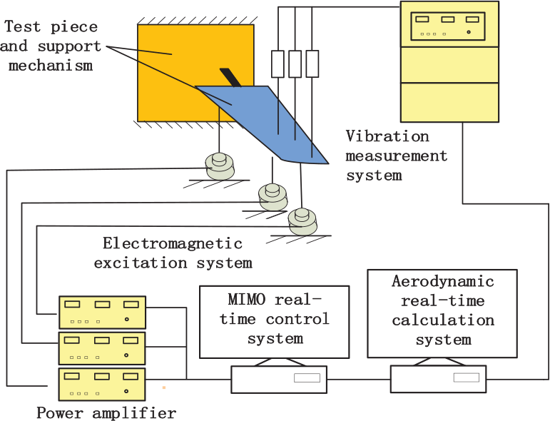
Figure 1. Diagram and blocks of the DWT test system.
2.1 Coupled dynamic model of the exciter system and test object
The structural dynamics of the test object can be expressed as
 \begin{equation}{{\textbf{\textit{M}}}\ddot{{\textbf{\textit{x}}}} }+ {\textbf{\textit{C}}}\ddot{{\textbf{\textit{x}}}}+{\textbf{\textit{K}}}\ddot{{\textbf{\textit{x}}}}={\textbf{\textit{f}}}\end{equation}
wherein M represents the mass matrix, C represents the damping matrix, K represents the stiffness matrix and f represents the force vector. Expanding the displacement according to the mode shape, we have
 \begin{equation}{\textbf{\textit{x}}}=\boldsymbol{\Phi q}\end{equation}
wherein Φ is the mode shape matrix and q is a generalised coordinate. Using equation (2) to apply a coordinate transformation, equation (1) becomes
 \begin{equation}\overline{{\textbf{\textit{M}}}}\ddot{{\textbf{\textit{q}}}} + \overline{{\textbf{\textit{C}}}}\ddot{{\textbf{\textit{q}}}}+ \overline{{\textbf{\textit{K}}}}{{\textbf{\textit{q}}}} = \overline{{\textbf{\textit{f}}}}\end{equation}
where  $\boldsymbol{\overline{M}=\boldsymbol{\Phi}^{T}M\boldsymbol{\Phi}}$,
  $\boldsymbol{\overline{C}={\boldsymbol{\Phi}}^{T}C\boldsymbol{\Phi}}$,
  $\boldsymbol{\overline{K}={\boldsymbol{\Phi}}^{T}K\boldsymbol{\Phi}}$ and
  $\boldsymbol{\overline{f}={\boldsymbol{\Phi}}^{T}f}$.
The electromagnetic exciter shown in Fig. 2 is mainly composed of an exciter moving coil, supporting spring, permanent magnet, shell and base. The permanent magnet, shell and base are fixed, while the moving coil is connected to the shell through the supporting spring. Its operating principle is as follows: an alternating current is introduced into the coil to generate a varying electromagnetic field; the magnetic field interacts with the permanent magnet to drive the moving coil, causing it to vibrate up and down.

Figure 2. Diagram of an electromagnetic exciter.
According to the operating principle of the exciter, its mechanical part can be regarded as a spring–mass system with a single degree of freedom(Reference Zhang, Zhang, Li, Ren and Han19), expressed by the following mathematical model:
 \begin{equation}m\ddot{x}^{\prime}+c\dot{x}^{\prime}+kx^{\prime}=f^{\prime}+f^{\prime\prime}\end{equation}
where m is the mass of the exciter moving coil plus the excitation rod (here, the excitation rod is assumed to be a rigid body), c is the damping of the exciter, k is the stiffness of the exciter support, f ′ is the reaction force of the excitation rod acting on the test piece and f ′′ is the electromagnetic force. The electromagnetic force satisfies the formula
 \begin{equation}f''=BlnI=K_{f}I\end{equation}
where B is the strength of the magnetic field, l is the length of the single-turn coil, n is the number of turns in the coil and I is the input current.
The dynamic equation for the current and voltage of the exciter drive coil can be written as
 \begin{equation}RI+L\frac{dI}{dt}+K_{v}\dot{x}^{\prime}=V^{\prime}\end{equation}
where R is the resistance of the coil, L is the self-inductance coefficient of the coil and the voltage across the coil is V′,  $K_{v}\dot{x}^{\prime}$ while is the self-inductance voltage and K v = K f.
The power amplification is equivalent to the system gain in a certain frequency band, which can be modelled mathematically as
 \begin{equation}V^{\prime}=G_{v}V\end{equation}
where V is the input voltage of the power amplifier and G V is the gain value.
2.2 Coupled dynamic model of the test object and exciter
In ground flutter testing, multiple exciters are required to simultaneously impose loads on the test object. Obviously, the vibration of the test object will affect the loading of the exciter force, and there is a strong coupling between the multiple exciters and the test object. For convenience of derivation, the degree of freedom of the structural dynamics of the test object is separated between excited and nonexcited points. Equation (2) can thus be written as
 \begin{equation}{\textbf{\textit{x}}} = \left[\begin{array}{c}
x_{s}\\[5pt]
x_{m}\end{array}\right] = \left[\begin{array}{c}
\boldsymbol{\Phi}_{s}\\[5pt]
\boldsymbol{\Phi}_{m}
\end{array}\right]{\textbf{\textit{q}}}\end{equation}
\begin{equation}{\textbf{\textit{x}}} = \left[\begin{array}{c}
x_{s}\\[5pt]
x_{m}\end{array}\right] = \left[\begin{array}{c}
\boldsymbol{\Phi}_{s}\\[5pt]
\boldsymbol{\Phi}_{m}
\end{array}\right]{\textbf{\textit{q}}}\end{equation}
where subscript s is the degree of freedom corresponding to nonexcited points, and subscript m is the degree of freedom corresponding to excited points. At the junction of the exciter and the test object, one must consider the double coordination condition for displacement and force:
 \begin{equation}\hspace*{14pt}{\textbf{\textit{x}}}_{m} = {\textbf{\textit{x}}}^{\prime}\end{equation}
 \begin{equation}{\textbf{\textit{f}}} + {\textbf{\textit{f}}}^{\prime}=0\end{equation}
Considering equations (3), (4), (6), and (7), we obtain
 \begin{align}
\left[\begin{array}{c@{\quad}c@{\quad}c}
{\overline{\textbf{\textit{M}}}}& 0&0 \\[4pt]
0 & {\textbf{\textit{m}}}&0\\[4pt]
0 & 0 & 0\end{array}\right]
\left[\begin{array}{c}
{\overline{\textbf{\textit{q}}}}\\[4pt]
{\ddot{\textbf{\textit{x}}}}\\[4pt]
\ddot{\textbf{\textit{I}}}\end{array}\right] +
\left[\begin{array}{c@{\quad}c@{\quad}c}
{\overline{\textbf{\textit{C}}}}& 0 & 0 \\[4pt]
0 & {\textbf{\textit{c}}} & 0\\[4pt]
0 & {\textbf{\textit{K}}}_{f} & {\textbf{\textit{L}}}\end{array}\right]
\left[\begin{array}{c}
\dot{\textbf{\textit{q}}}\\[4pt]
\dot{\textbf{\textit{x}}^{\prime}}\\[4pt]
\dot{\textbf{\textit{I}}}\end{array}\right] +
\left[\begin{array}{c@{\quad}c@{\quad}c}
{\overline{\textbf{\textit{K}}}} & 0 & 0 \\[4pt]
0 & {\textbf{\textit{k}}} & - {\textbf{\textit{k}}}_{\textbf{\textit{f}}}\\[4pt]
0 & 0 & {\textbf{\textit{R}}}\end{array}\right]
\left[\begin{array}{c}
{\textbf{\textit{q}}}\\[4pt]
{{\textbf{\textit{x}}}^{\prime}}\\[4pt]
{\textbf{\textit{I}}}\end{array}\right] =
\left[\begin{array}{c}
{\overline{\textbf{\textit{f}}}}\\[4pt]
{\overline{\textbf{\textit{f}}}}^{\prime}\\[4pt]
{\textbf{\textit{GV}}}\end{array}\right].\nonumber\\
\end{align}
\begin{align}
\left[\begin{array}{c@{\quad}c@{\quad}c}
{\overline{\textbf{\textit{M}}}}& 0&0 \\[4pt]
0 & {\textbf{\textit{m}}}&0\\[4pt]
0 & 0 & 0\end{array}\right]
\left[\begin{array}{c}
{\overline{\textbf{\textit{q}}}}\\[4pt]
{\ddot{\textbf{\textit{x}}}}\\[4pt]
\ddot{\textbf{\textit{I}}}\end{array}\right] +
\left[\begin{array}{c@{\quad}c@{\quad}c}
{\overline{\textbf{\textit{C}}}}& 0 & 0 \\[4pt]
0 & {\textbf{\textit{c}}} & 0\\[4pt]
0 & {\textbf{\textit{K}}}_{f} & {\textbf{\textit{L}}}\end{array}\right]
\left[\begin{array}{c}
\dot{\textbf{\textit{q}}}\\[4pt]
\dot{\textbf{\textit{x}}^{\prime}}\\[4pt]
\dot{\textbf{\textit{I}}}\end{array}\right] +
\left[\begin{array}{c@{\quad}c@{\quad}c}
{\overline{\textbf{\textit{K}}}} & 0 & 0 \\[4pt]
0 & {\textbf{\textit{k}}} & - {\textbf{\textit{k}}}_{\textbf{\textit{f}}}\\[4pt]
0 & 0 & {\textbf{\textit{R}}}\end{array}\right]
\left[\begin{array}{c}
{\textbf{\textit{q}}}\\[4pt]
{{\textbf{\textit{x}}}^{\prime}}\\[4pt]
{\textbf{\textit{I}}}\end{array}\right] =
\left[\begin{array}{c}
{\overline{\textbf{\textit{f}}}}\\[4pt]
{\overline{\textbf{\textit{f}}}}^{\prime}\\[4pt]
{\textbf{\textit{GV}}}\end{array}\right].\nonumber\\
\end{align}
Due to the multi-point excitation, the physical parameters associated with the exciter become diagonal matrices.
It can be shown from equations (8) and (9) that
 \begin{equation}{\boldsymbol{\Phi}}_{m}{\textbf{\textit{q}}} = {\textbf{\textit{x}}}'.\end{equation}
Substituting equation (12) into (11), rearranging and then considering equation (10), the following equation is obtained:
 \begin{align}
&\left[\begin{array}{c@{\quad}c}
{\overline{\textbf{\textit{M}}}}+ {\boldsymbol{\Phi}}_{m}^{T}\, {\textbf{\textit{m}}}{\boldsymbol{\Phi}}_{m} & 0 \\[6pt]
0 & 0 \\[6pt]
\end{array}\right]
\left[\begin{array}{c}
\ddot{\textbf{\textit{q}}}\\[9pt]
\ddot{\textbf{\textit{I}}}
\end{array}\right] +
\left[\begin{array}{c@{\quad}c}
{\overline{\textbf{\textit{C}}}}+ {\boldsymbol{\Phi}}_{m}^{T}\, \textbf{\textit{c}}{\boldsymbol{\Phi}}_{m} & 0 \\[6pt]
{\boldsymbol{\Phi}}_{m} {\textbf{\textit{K}}}_{f} & {\textbf{\textit{L}}}
\end{array}\right] +
\left[\begin{array}{c}
\dot{\textbf{\textit{q}}}\\[6pt]
\dot{\textbf{\textit{I}}}\end{array}\right]\nonumber\\[10pt]
&\qquad +
\left[\begin{array}{c@{\quad}c}
{\overline{\textbf{\textit{K}}}}+ {\boldsymbol{\Phi}}_{m}^{T} {\textbf{\textit{k}}}{\boldsymbol{\Phi}}_{m} & -{\boldsymbol{\Phi}}_{m}^{T} {\boldsymbol{K}}_{f}\\[6pt]
0 & {\textbf{\textit{R}}}\\[6pt]
\end{array}\right]
\left[\begin{array}{c}
\textbf{\textit{q}}\\[6pt]
\textbf{\textit{I}}\end{array}\right] =
\left[\begin{array}{c}
0\\[6pt]
G{\textbf{\textit{V}}}\end{array}\right]\end{align}
\begin{align}
&\left[\begin{array}{c@{\quad}c}
{\overline{\textbf{\textit{M}}}}+ {\boldsymbol{\Phi}}_{m}^{T}\, {\textbf{\textit{m}}}{\boldsymbol{\Phi}}_{m} & 0 \\[6pt]
0 & 0 \\[6pt]
\end{array}\right]
\left[\begin{array}{c}
\ddot{\textbf{\textit{q}}}\\[9pt]
\ddot{\textbf{\textit{I}}}
\end{array}\right] +
\left[\begin{array}{c@{\quad}c}
{\overline{\textbf{\textit{C}}}}+ {\boldsymbol{\Phi}}_{m}^{T}\, \textbf{\textit{c}}{\boldsymbol{\Phi}}_{m} & 0 \\[6pt]
{\boldsymbol{\Phi}}_{m} {\textbf{\textit{K}}}_{f} & {\textbf{\textit{L}}}
\end{array}\right] +
\left[\begin{array}{c}
\dot{\textbf{\textit{q}}}\\[6pt]
\dot{\textbf{\textit{I}}}\end{array}\right]\nonumber\\[10pt]
&\qquad +
\left[\begin{array}{c@{\quad}c}
{\overline{\textbf{\textit{K}}}}+ {\boldsymbol{\Phi}}_{m}^{T} {\textbf{\textit{k}}}{\boldsymbol{\Phi}}_{m} & -{\boldsymbol{\Phi}}_{m}^{T} {\boldsymbol{K}}_{f}\\[6pt]
0 & {\textbf{\textit{R}}}\\[6pt]
\end{array}\right]
\left[\begin{array}{c}
\textbf{\textit{q}}\\[6pt]
\textbf{\textit{I}}\end{array}\right] =
\left[\begin{array}{c}
0\\[6pt]
G{\textbf{\textit{V}}}\end{array}\right]\end{align}
For brevity, let  $\boldsymbol{\tilde{M}=\overline{M}+{\boldsymbol{\Phi}}^{T}_{m}m{\boldsymbol{\Phi}}_{m}}$,
  $\boldsymbol{\tilde{C}=\overline{C}+{\boldsymbol{\Phi}}_{m}^{T}c{\boldsymbol{\Phi}}_{m}}$ and
  $\boldsymbol{\tilde{K}=\overline{K}+{\boldsymbol{\Phi}}_{m}^{T}k{\boldsymbol{\Phi}}_{m}}$. Equation (14) is then obtained from the first set of equations (13),
 \begin{equation}\boldsymbol{\ddot{q}}= - \boldsymbol{\tilde{M}}^{-1}\boldsymbol{\tilde{C}\ddot{q}}-\tilde{\textbf{\textit{M}}}^{-1}\boldsymbol{\tilde{K}q}+\boldsymbol{\tilde{M}}^{-1}{\boldsymbol{\Phi}}_{m}^{T}K_{f}I_{i}\end{equation}
Meanwhile, equation (13) can be further transformed into the following state-space form:
 \begin{equation}
\left[\begin{array}{c}
{\ddot{\textbf{\textit{q}}}}\\[5pt]
{\dot{\textbf{\textit{q}}}}\\[5pt]
{\dot{\textbf{\textit{I}}}} \end{array}\right] =
\left[\begin{array}{c@{\quad}c@{\quad}c}
{\tilde{-\textbf{\textit{M}}}}^{-1}\tilde{\textbf{\textit{C}}} & {\tilde{-\textbf{\textit{M}}}^{-1}\tilde{\textbf{\textit{K}}}} & {\tilde{-\textbf{\textit{M}}}^{-1}\boldsymbol{\Phi}_{m}^{T}{\textbf{\textit{K}}}_{f}}\\[5pt]
\textbf{\textit{E}} & 0 &0\\[5pt]
{\tilde{-\textbf{\textit{L}}}^{-1}{\textbf{\textit{K}}}_{f}\boldsymbol{\Phi}_{m}} & 0 & {-\textbf{\textit{L}}^{-1}\textbf{\textit{R}}}\end{array}\right]
\left[\begin{array}{c}
{\dot{\textbf{\textit{q}}}}\\[5pt]
{{\textbf{\textit{q}}}}\\[5pt]
{{\textbf{\textit{I}}}}\end{array}\right] +
\left[\begin{array}{c}
0\\[5pt]
0\\[5pt]
{\textbf{\textit{L}}^{-1}G}\end{array}\right]\textbf{\textit{V}}
\end{equation}
\begin{equation}
\left[\begin{array}{c}
{\ddot{\textbf{\textit{q}}}}\\[5pt]
{\dot{\textbf{\textit{q}}}}\\[5pt]
{\dot{\textbf{\textit{I}}}} \end{array}\right] =
\left[\begin{array}{c@{\quad}c@{\quad}c}
{\tilde{-\textbf{\textit{M}}}}^{-1}\tilde{\textbf{\textit{C}}} & {\tilde{-\textbf{\textit{M}}}^{-1}\tilde{\textbf{\textit{K}}}} & {\tilde{-\textbf{\textit{M}}}^{-1}\boldsymbol{\Phi}_{m}^{T}{\textbf{\textit{K}}}_{f}}\\[5pt]
\textbf{\textit{E}} & 0 &0\\[5pt]
{\tilde{-\textbf{\textit{L}}}^{-1}{\textbf{\textit{K}}}_{f}\boldsymbol{\Phi}_{m}} & 0 & {-\textbf{\textit{L}}^{-1}\textbf{\textit{R}}}\end{array}\right]
\left[\begin{array}{c}
{\dot{\textbf{\textit{q}}}}\\[5pt]
{{\textbf{\textit{q}}}}\\[5pt]
{{\textbf{\textit{I}}}}\end{array}\right] +
\left[\begin{array}{c}
0\\[5pt]
0\\[5pt]
{\textbf{\textit{L}}^{-1}G}\end{array}\right]\textbf{\textit{V}}
\end{equation}
where E represents the unit matrix. The physical quantities required for a ground flutter test system are the displacement, velocity and acceleration response of the test object, which can be solved using equation (15), then directly obtained according to equation (8). In addition, a ground flutter test system also needs to obtain the dynamic forces that the exciter applies to the test object, so the real-time MIMO controller is designed in the next section. We look again at the second set of equations in equation (11):
 \begin{equation}\boldsymbol{f^{\prime}}=\boldsymbol{m\Phi}_{m}\ddot{\textbf{\textit{q}}}+\boldsymbol{c\Phi}_{m}\dot{\textbf{\textit{q}}}+ \boldsymbol{k\Phi_{m}}{\textbf{\textit{q}}}-\boldsymbol{K}_{f}{\textbf{\textit{I}}}\end{equation}
Considering that the force applied by the exciter to the test object and f ′ are reaction forces, equation (14) now yields
 \begin{equation}
\boldsymbol{f}=
\left[\begin{array}{c}
\textbf{\textit{m}}\boldsymbol{\Phi}_{{m}}\tilde{\textbf{\textit{M}}}^{-1}\tilde{\textbf{\textit{C}}}-\textbf{\textit{c}}\boldsymbol{\Phi}_{m}\\[5pt]
{\textbf{\textit{m}}\boldsymbol{\Phi}_{m}\tilde{\textbf{\textit{M}}}^{-1}\tilde{\textbf{\textit{K}}}-\textbf{\textit{k}}\boldsymbol{\Phi}_{m}}\\[5pt]
{-\textbf{\textit{m}}}\boldsymbol{\Phi}_{m}\tilde{\textbf{\textit{M}}}^{-1}\boldsymbol{\Phi}_{m}^{T}\textbf{\textit{K}}_{f}+\textbf{\textit{K}}_{f}\\
\end{array}\right]
\left[\begin{array}{c}
{\dot{\textbf{\textit{q}}}}\\[5pt]
{\textbf{\textit{q}}}\\[5pt]
{\textbf{\textit{I}}}\end{array}\right]
\end{equation}
\begin{equation}
\boldsymbol{f}=
\left[\begin{array}{c}
\textbf{\textit{m}}\boldsymbol{\Phi}_{{m}}\tilde{\textbf{\textit{M}}}^{-1}\tilde{\textbf{\textit{C}}}-\textbf{\textit{c}}\boldsymbol{\Phi}_{m}\\[5pt]
{\textbf{\textit{m}}\boldsymbol{\Phi}_{m}\tilde{\textbf{\textit{M}}}^{-1}\tilde{\textbf{\textit{K}}}-\textbf{\textit{k}}\boldsymbol{\Phi}_{m}}\\[5pt]
{-\textbf{\textit{m}}}\boldsymbol{\Phi}_{m}\tilde{\textbf{\textit{M}}}^{-1}\boldsymbol{\Phi}_{m}^{T}\textbf{\textit{K}}_{f}+\textbf{\textit{K}}_{f}\\
\end{array}\right]
\left[\begin{array}{c}
{\dot{\textbf{\textit{q}}}}\\[5pt]
{\textbf{\textit{q}}}\\[5pt]
{\textbf{\textit{I}}}\end{array}\right]
\end{equation}
The state-space equation consisting of equations (15) and (17) can be used directly in the design of robust MIMO dynamic force controllers.
2.3 Robust dynamic force control of the vibration exciter
Compared with numerical flutter predictions, there are more uncertainties in the coupled exciter–test model–controller–sensors coupled system. As one of the popular uncertain robust control methods, the MIMO H ∞ method can be applied to design such control laws. The mixed sensitivity method is used to design the H ∞-robust controller of the dynamic force to the excitation system, which can be transformed into a standard control problem as shown in Fig. 3.

Figure 3. Control block of H ∞-optimal control method.
The optimal control problem with the excitation system as the controlled object can be described as follows:
 \begin{equation}
\text{min}_{K}
\left||\begin{array}{c}
W_{P}S\\[5pt]
W_{U}KS\\[5pt]
W_{G}T\end{array}\right||_{\infty}
\end{equation}
\begin{equation}
\text{min}_{K}
\left||\begin{array}{c}
W_{P}S\\[5pt]
W_{U}KS\\[5pt]
W_{G}T\end{array}\right||_{\infty}
\end{equation}
where W PS is the transfer function of the external input to the controlled output z 1, which can be regarded as the weighted output of the error signal e, thus representing the anti-interference ability of the system. W UKS is the transfer function of the external input to the controlled output z 2, which can be regarded as the weighted output of the control input u, and also as the additive uncertainty output of the controlled object G. Therefore, it represents the restrictive effect on the amplitude of the control signal on the controller, as well as the robustness of the control system in the case of additive uncertainty. W GT is the transfer function of the external input to the controlled output z 3, which can be regarded as the multiplicative uncertainty output of the controlled object. It thus represents the robust stability of the control system in the case of multiplicative uncertainty.
The selection of the weighting functions  $W_{P}(s)$, W U(s) and W G(s) is the key issue when designing a robust controller. The greater the amplitude of W P(s), the higher the control accuracy of the control system. However, an excessive W P(s) will make it more difficult to realise the control system. Generally, the amplitude is larger in the operating frequency range set by the controller, but smaller outside this range to ensure that the control system achieves good tracking characteristics. Adjusting W U(s) will affect the control signal. The weighted function can be adjusted to prevent saturation of the control voltage. W G(s) is the robust weighted function matrix of the system. It is determined by the non-structural uncertainty of the model, comprising the high-frequency unmodeled dynamics and the uncertainty of the model parameters. Here, note that W P(s) and W G(s) are generally complementary, that is, where W P(s) is large, W G(s) should be smaller, while W G(s) should be larger if W P(s) is smaller.
2.4 Fast calculation of the unsteady aerodynamic forces
For a ground flutter test system, the aerodynamic force must be calculated in real time according to the structural response of the test object. At present, in ground flutter testing systems, engineering aerodynamic models are usually applied(Reference Zeng, Kingsbury, Ritz, Chen, Lee and Mignolet8,Reference Xu, Wu and Yang10,Reference Song11) , such as the dipole grid method, ZONA6, ZONA7 and so on. For an aeroelastic problem, the unsteady aerodynamic forces are calculated as
 \begin{equation}\boldsymbol{f}=q_{\infty}\boldsymbol{G}^{T}\boldsymbol{A}(ik)\boldsymbol{Gx}\end{equation}
where q ∞ is the dynamic pressure, G is the interpolation transformation matrix, A is the aerodynamic influence coefficient matrix, k is the reduction frequency,  $k=\omega L/V$, Ω is the resonant circular frequency, L is the reference length and V is the flight speed. For convenience, the aeroelastic analysis is performed in a modal generalised coordinate system. The generalised aerodynamic model is
 \begin{equation}
{\overline{\boldsymbol{f}}} = q_{\infty}{\boldsymbol{\Phi}^{T}\textbf{\textit{G}}^{T}}{\textbf{\textit{A}}}(ik){\textbf{\textit{G}}\boldsymbol{\Phi} \textbf{\textit{q}}}\end{equation}
\begin{equation}
{\overline{\boldsymbol{f}}} = q_{\infty}{\boldsymbol{\Phi}^{T}\textbf{\textit{G}}^{T}}{\textbf{\textit{A}}}(ik){\textbf{\textit{G}}\boldsymbol{\Phi} \textbf{\textit{q}}}\end{equation}
For the engineering aerodynamic model, the aerodynamic influence coefficient matrix is generally expressed in the frequency domain, which must be extended to the Laplace domain and then written in state-space form(Reference Gao, Tan and Pu20). The general expression for the minimum state method rational function fitting is
 \begin{equation}\boldsymbol{\overline{Q}}(s)=\boldsymbol{\overline{A}}_{0}+\frac{L}{V}\boldsymbol{\overline{A}}_{1}s+\frac{L^{2}}{V^{2}}\boldsymbol{\overline{A}}_{2}s^{2}+\overline{\textbf{\textit{D}}}\left(\overline{\textbf{\textit{E}}}s-\frac{V}{L}\overline{\textbf{\textit{R}}}\right)^{-1}\overline{\boldsymbol{E}}s\end{equation}
where  $\boldsymbol{Q}(s)=\boldsymbol{\Phi}^{T}{\textbf{\textit{G}}}^{T}\textbf{\textit{A}}(ik)\textbf{\textit{G}}\boldsymbol{\Phi}$,
  $s=ik$,
  $\boldsymbol{\overline{A}}_{0}$,
  $\boldsymbol{\overline{A}}_{1}$,
  $\boldsymbol{\overline{A}}_{2}$,
  $\boldsymbol{\overline{D}}$ and
  $\boldsymbol{\overline{E}}$ are matrices obtained by fitting, while
  $\boldsymbol{\overline{R}}$ is a diagonal matrix that is used to indicate the hysteresis state of the model caused by the hysteresis effect of the unstable airflow. The performance of the inverse Laplace transformation on equation (21) yields a time-domain calculation model whose input is the generalised response and whose output is the generalised aerodynamic force. The model is shown in Fig. 4.

Figure 4. Control block model of generalised aerodynamic forces.
3.0 EXCITATION/MEASUREMENT POINT OPTIMISATION METHOD
In a ground flutter test, only a finite number of points can be excited and measured, resulting in an optimisation problem to define the location of the excitation and measurement points. Aiming to achieve the minimum difference between the flutter speed and the flutter frequency in reference 8, an optimisation method for the excitation and measurement points is presented here. In reference 10, to minimise the difference between the original mode and the interpolated mode of the critical flutter mode, a genetic algorithm was applied as the optimisation search method to define the optimal aerodynamic reduction position. Herein, according to the effective independent method(Reference Cheng, Yan, Chen, He and Zhang21), the Fisher information matrix is applied in the optimisation of the excitation and measurement points. From equation (2), an effective unbiased estimate of the modal coordinate q is obtained as
 \begin{equation}\boldsymbol{\hat{q}}=[\boldsymbol{\Phi}^{T}\boldsymbol{\Phi}]^{-1}\boldsymbol{\Phi}^{T}\boldsymbol{U}\end{equation}
where U is the measurement information from the sensor. Considering the measurement noise, this becomes
 \begin{equation}\boldsymbol{U}=\boldsymbol{\Phi}\boldsymbol{q}+\boldsymbol{N}\end{equation}
where N represents white noise with variance  $\sigma^{2}$. The covariance matrix of the estimate is
 \begin{equation}\boldsymbol{P}=\boldsymbol{E}\left[(\boldsymbol{q-\hat{q}}) (\boldsymbol{q-\hat{q}})^{T}\right]=\boldsymbol{Q}^{-1}\end{equation}
 \begin{equation}\boldsymbol{Q} = \frac{1}{\boldsymbol{\sigma}^{2}}\boldsymbol{\Phi}^{T}\boldsymbol{\Phi}\end{equation}
where Q is the Fisher information matrix. When the Fisher information matrix Q is maximised, the covariance of the estimates is the smallest. This will result in an optimal estimate for the modal coordinate q. Kammer(Reference Kammer22) proposed an efficient independent method to maximise the Fisher information matrix Q.
The equal power matrix is constructed as
 \begin{equation}\boldsymbol{E}=\boldsymbol{\Phi}[\boldsymbol{\Phi}^{T}\boldsymbol{\Phi}]^{-1}\boldsymbol{\Phi}^{T}\end{equation}
Where the magnitude of the diagonal element value of E represents the linear independent contribution of the candidate point to the corresponding sensor vias the modal matrix. By sorting the diagonal elements of the E matrix, then deleting the smallest value iteratively, the last j points are the optimal measuring points for the ground flutter test system. Using these finite number of points, an optimal estimate for the modal coordinates can be obtained. Equation (22) is then rewritten as
 \begin{equation}\boldsymbol{\hat{q}}=[\boldsymbol{\Phi}^{T}_{j}\boldsymbol{\Phi}_{j}]^{-1}\boldsymbol{\Phi}^{T}_{j}\boldsymbol{U}\end{equation}
where  $\boldsymbol{\Phi}_{j}$ is the mode shape matrix corresponding to the degree of freedom of the j optimal points.
If the best estimate for the response of the coordinate of the main mode can be obtained from the response measured at a finite number of points, the generalised force is completely equivalent. Complete equivalence is then achieved in theory between the measurement and excitation at the finite number of points. When the excitation point is selected the same as the measurement point, the excitation force to be applied to the test piece based on the generalised force equivalent principle is
 \begin{equation}\boldsymbol{f^{\prime}_{j}}=[\boldsymbol{\Phi}_{j}\boldsymbol{\Phi}_{j}^{T}]^{-1}\boldsymbol{\Phi}_{j}\,\boldsymbol{\overline{f}}\end{equation}
4.0 NUMERICAL VALIDATION AND DISCUSSION
4.1 Model description
The test object model is a trapezoidal aluminium plate. The length of the root chord is 2.54m, the length of the tip chord is 1.27m and the length of the semi-span is 2.54m. The support structure is located at one-third of the root of the model. The structural finite element model is shown in Fig. 5. The plate has a total number of 100 nodes and 81 shell elements. The support structure has a total number of nine nodes and nine beam elements. The support end constrains all six degrees of freedom, while the structural nodes constrain one and six degrees of freedom.

Figure 5. Finite element model of flat plate.
The parameters for the excitation system model include the mass of the exciter moving coil m, the damping c, the stiffness k, the electromagnetic constant k f, the coil resistance R, and the inductance L as shown in Table 1. The model parameters refer to the selected exciters applied in the experimental DWT system.
4.2 Finite measurement/excitation point optimisation
The effective independent method is used to optimise the arrangement of the finite number of points for the above-described model. The measurement points are taken to be the same as the excitation points. The optimal arrangements for the cases with two to five points are shown in Fig. 6. The Fisher matrices were constructed to determine the excitation and measurement points. Because there are more than 600 Degrees of Freedom (DOFs) in this case, the Fisher matrix is very large, with dimension of more than 600 by 600. To simply the description of the designed Fisher matrix, only the largest few values of the Fisher matrix are given; For example, the matrix values of the five vertical DOFs of the five points P1 to P5 optimised in Fig. 6(d) were 0.9753, 0.9521, 0.9194, 0.8294 and 0.3515, respectively.

Figure 6. Locations of optimised points for different selected models.
After the construction of the Fisher matrix, the optimised points are then applied to the modal response estimates so that the aeroelastic analysis can be carried out. Here we used the benchmark example of NASTRAN/ZONA6 to verify the effectiveness of the proposed method for DWT. In the numerical simulation, the ZONA6 aerodynamic model was used. The frequency-domain aerodynamic model is transformed into a time-domain model by using the minimum state method. The critical flutter speeds were calculated at several Mach numbers by NASTRAN and using the proposed method with the model including five optimisation points. A comparison of the flutter speeds predicted at different Mach numbers when using both NASTRAN and the presented method is presented in Fig. 7. It seems that the flutter speed predicted by the proposed generalised force equivalence-based method agrees well with those obtained using NASTRAN. This finding indicates that the generalised force equivalence-based flutter prediction method is accurate enough to be applied as the flutter calculation solver in the DWT system.

Figure 7. Flutter speeds predicted by NASTRAN and the proposed method at different Mach numbers.
To determine the effect of the number of measurement/excitation points on the flutter speed calculation, the critical flutter speed was calculated for cases with different numbers of measurement/excitation points. The predicted errors are shown in Fig. 8, revealing that the error on the critical flutter speed obtained by the generalised force equivalent method is very small. The maximum error is less than 1% even only for the case with only two points. As the number of points is increased, the error decreases very fast and the result approaches the predicted theoretical value. From the structural dynamics perspective, the number of measurement/excitation points can theoretically be equivalent to the number of modal equations. For the aeroelastic model shown in Fig. 9, flutter is mainly caused by the first-order bending and second-order torsional modes. The first two modes can be used to describe the dominant flutter behaviour to some extent, obtaining good results even if only two points are used. As the number of points is increased, the available modal information will become more complete, so that the calculation results will approach the theoretical value. From Fig. 8, it can be concluded that, for the aeroelastic model shown in Fig. 5, the predicted errors become very small but reduce very slowly for numbers above four. The use of four points is thus a relatively good choice for DWT test systems.

Figure 8. Errors on flutter speed predicted using different numbers of sensors and exciters.

Figure 9. Aeroelastic model with measurement noise.
The discussion above considered a relatively ideal state, that is, where the modal vibration mode, measurement data, etc. all have ideal values without interference from noise. However, in real-life engineering applications, due to the influence of measurement noise and the modal identification method, certain deviations from the measurement point data and mode shape will occur. To validate the performance of the proposed method in an uncertain environment, a random mode noise interference source was introduced into the modal vibration mode data and the measurement point data in the flutter calculation procedure. The aeroelastic model with measurement noise is shown in Fig. 9. Its accuracy at Mach number 0.8 was analysed under different magnitudes of interference.
Table 2 presents the flutter speeds predicted by the generalised force equivalence-based modelling method for the aeroelastic model shown in Fig. 5 with different numbers of points and different magnitudes of noise interference. A reference flutter speed of 259 m/s is predicted by NASTRAN without noise interference at a Mach number of 0.8. As seen from Table 2, the theoretic approach using only two points can already achieve good results, although the noise has a great influence on the accuracy. As the number of points is increased, the anti-interference performance is enhanced. The maximum error is less than 1.20% for the 10% noise level when using the four-point model, and less than 1% when using the five-point model. These result indicate that the generalised force equivalence-based aeroelastic modelling method achieves good accuracy and sufficient robustness, which is very important for practical DWT systems.
Table 1 Model parameters of exciter
Table 2 Flutter speed results for different numbers of points and measurement noise levels (Reference value 259, predicted by NASTRAN without noise)

From the viewpoint of numerical simulations, more points could be selected. However, the use of more exciters requires higher-order controllers and more complex hardware systems, while the resulting increase in prediction accuracy is not so obvious. The use of an excessive number of excitation/measurement points can also cause inconvenience when performing real tests. It will lead to an increase in the order of the aerodynamic calculation model and also increase the calculation time delay of each closed loop. On the other hand, it is also necessary to increase the corresponding measuring equipment, excitation equipment and control channel, thus making the experiment more complicated. Based on comprehensive consideration of all these effects, a good choice is to use four measurement/excitation points, both to achieve good accuracy and to avoid the requirement for expensive experimental test systems for engineering applications.
4.3 Control performance of the excitation system
To analyse the influence of the accuracy of the exciter model parameters on the control system, the feedback control system model shown in Fig. 10 was constructed. In this case, the number of excitation/measurement points is four.

Figure 10. Schematic of feedback control system model for excitation system.
When designing the controller, W P selects an eighth-order Butterworth bandpass filter with a frequency band of 5–20Hz and gain of 10. W U takes a constant gain of 0.05, and W G takes a constant gain of 0.1. Measurement noise interference of 10% is applied in the feedback blocks. A sinusoidal reference signal is applied to one channel, while the input reference signals from the other channels are zero. The results of the control simulation are shown in Fig. 11.

Figure 11. Output force signals of different points to input control signals of different exciters.
As seen from Fig. 11, only when a sinusoidal reference signal is applied to a certain channel can the output signal of the channel track the input reference signal well. Meanwhile, the rest of the channel outputs are close to zero, which indicates that the input of the current channel has no effect on the output of the other channels, achieving decoupling between the different channels. Moreover, the controller exhibits certain robustness, and the tracking control of the force signal and the decoupling between the different channels are achieved even in the presence of feedback noise interference. We further analyse the influence of the model parameters on the control accuracy. The system performance indicators can be calculated from the following equation based on the error signal:
 \begin{equation}{\textbf{\textit{error}}}=\boldsymbol{\int}^{\boldsymbol{\infty}}_{0}|\boldsymbol{e(t)}|\boldsymbol{dt}\end{equation}
In the simulation process, the variation of the system index with a certain parameter can be obtained by changing the value of a certain exciter parameter, such that sensitivity of the parameter near its nominal value is obtained; the sensitivity of the exciter parameter is obtained as shown in Fig. 12.

Figure 12. Sensitivities of exciter model parameters.
It is seen from this figure that the electrical parameters generally have a greater influence on the control performance than do the mechanical parameters such as the mass, damping and stiffness. In particular, the electromagnetic constant k f and resistance R show the highest sensitivity, and the accuracy of these two parameters has the greatest influence on the performance of the control system. Therefore, when constructing a ground flutter test system with the proposed method for the controller design, the measurement accuracy of the electromagnetic constant k f and resistance R should be improved to reduce the influence of parameter uncertainty on the control accuracy.
4.4 System simulation performance
Having established and validated the accuracy of each sub-system, the whole system co-simulation analysis can be carried out. The calculation process is shown in Fig. 13.

Figure 13. System-level simulation model for whole DWT system.
In this system-level simulation process, the influence of noise on the generalised modal coordinate response estimation and the time delay effect of the excitation force real-time control are considered, while the error on the critical flutter speed is also analysed (Fig. 14). The noise level indicates the measurement noise levels applied to the sensors.

Figure 14. Error in cases with different time delays and measurement noise levels.
Figure 14 confirms that the influence of the noise and the control delay of the generalised modal coordinate response estimation on the critical flutter speed cannot be ignored. Regarding the control delay, the existence of a time delay will cause the critical flutter speed to become smaller. Especially when the time delay increases to a certain extent, the error will suddenly become very large. Therefore, it is particularly important to pay attention to the influence of such time delay on the accuracy of ground flutter test systems; For example, real-time hardware devices and real-time algorithms are required for physical DWT systems.
5.0 EXPERIMENTAL TEST AND VALIDATION
In this section, we further validate the proposed generalised force equivalence modelling method via an experimental test. As the first step, the exicter–plant coupled model is first evaluated. The DWT test system is shown in Fig. 15. The clamped plate has a length of 1.2m, a width of 0.7m and a thickness of 0.005m. The mode shape  $\boldsymbol{\Phi}$, modal mass
  $\boldsymbol{\overline{M}}$, modal damping
  $\boldsymbol{\overline{C}}$ and modal stiffness
  $\boldsymbol{\overline{K}}$ were obtained from the plate mode test. The model parameters for the selected standard exciters were obtained from the test identification. The details of the model parameters are presented in Table 3.
Table 3 Model parameters of exciter

Figure 15. Exciter–plate coupled test model in DWT test system.

Figure 16. The output forces predicted by numerical simulation and experimental test.

Figure 17. Vibration signals of plate at two different velocities.
During the test verification, 5–100Hz sine-wave sweep signals were applied to the exciters, then the exciting forces of the exciters were measured separately. A comparison of the measured force and that predicted by the coupled dynamic model for exciters 1 and 2 is shown in Fig. 16, revealing good agreement between the test and simulation results in both the time- and frequency domain. The main vibration frequency error is less than 1%, while the amplitude error is less than 1.5%, indicating that the proposed exciter–plate coupled dynamic model offers sufficient accuracy to further predict the flutter.
The flutter velocity predicted by the DWT test system was then evaluated for different flow speeds. When the flow velocity parameter was 207m/s, Fig. 17 reveals that the vibration of the plate was in a positive damping state under a small disturbance. However, when the velocity was increased to 213m/s, the vibration system appears to diverge. The critical flutter velocity of the test plate should thus lie between 207m/s and 213m/s. The flutter velocity predicted by the ZONA/NASTRAN solver was 203.88m/s. This indicates that the maximum error between the DWT system and the numerical simulation was less than 4.5%, being sufficiently good and acceptable for engineering applications. The experimental test results further validate the accuracy and feasibility of the modelling method proposed herein.
6.0 CONCLUSIONS
A new parameterised modelling and design method for DWT flutter test systems based on the generalised force equivalence method is proposed. In the proposed DWT co-simulation framework, the generalised structural dynamic model, the exciter–electric coupling dynamics model and the double, force and displacement coordination conditions at the interface between the test piece and electromagnetic excitation devices are taken into consideration. The feasibility and accuracy of the proposed system-level numerical DWT model were validated by considering a plate model with four exciters/transducers.
(1) Firstly, the proposed parametric coupling dynamic model for the DWT flutter system is very convenient to analyse the influence of model parameter disturbance, measurement noise and control delay on the system accuracy.
-
(2) Secondly, by introducing the Fisher information matrix into the optimisation of the excitation/measurement points, there is no need to apply complex methods or iterative procedures to search for the minimum value. Rather, only some simple matrix calculations are required.
-
(3) Finally, by introducing the generalised force equivalence method, the best estimate of the main mode coordinate response can be obtained from the response measured at a finite number of points. This enables the proposed parameterisation model to show good anti-uncertainty performance against control time delays and measurement noise, which is one of key issues in the design and testing of real experimental DWT system.
ACKNOWLEDGEMENT
This work was partially supported by the National Natural Science Foundation of China (nos. 11872293 and 11672225), the Open Foundation of the Science and Technology on Reliability and Environment Engineering Laboratory (No. 6142004190307) and international collaboration program no. B18040.


