


NOMENCLATURE
- dA
area of a span-wise wing strip
- ci
local chord
- ci
unit vector in the direction of the chord
- Cd
drag coefficient of the strip aerofoil
- CD
lifting surface drag coefficient
- Cl
lift coefficient of the strip aerofoil
- CL
lifting surface lift coefficient
- Cm
pitching moment coefficient about the quarter-chord point of the strip aerofoil
- CM
lifting surface pitching moment coefficient about the quarter-chord of the root chord
- F
aerodynamic force generated by a lifting surface
- k
reduced frequency
- K decay
constant that reflects the rate at which the circulation decays with time
- dl
differential segment along the lifting surface quarter-chord line
- M
aerodynamic moment generated by a lifting surface
- ni
unit vector normal to the aerofoil chord
- r 0
length of the vortex segment
- r 1, r 2
moduli of the spatial vectors
- r1, r2
vectors from the starting and ending points of a vortex segment to the arbitrary point in space
- ri
vector from a reference point to the middle of the quarter-chord vortex segment
- R i
component of the non-linear system residual vector
- Rϕ, Rθ, Rψ
rotation matrices corresponding to the euler angles
- Δt
time step
- vrel
additional velocity due to lifting surface motion relative to its body-fixed frame
- V ∞
modulus of the freestream velocity
- V
local velocity vector
- V0
velocity of the body-fixed frame origin point
- w
velocity induced by a straight vortex segment
- (x, y, z)
coordinates in the body-fixed reference frame
- (X, Y, Z)
coordinates in the inertial reference frame
- (X 0, Y 0, Z 0)
coordinates of the body-fixed frame origin point with respect to the inertial frame
- α
lifting surface angle-of-attack
- αi
local effective angle-of-attack
- Γ
circulation
- Γ0
original circulation of a vortex ring, at the time step when it was shed into the wake
- δ
cut-off radius
- ε
convergence criterion
- ρ
air density
- Δτ
fictitious time step
- (ϕ, θ, ψ)
Euler Angles
- ω
angular frequency
- Ω
angular velocity of the body-fixed frame
1.0 INTRODUCTION
Since its original development almost a century ago(Reference Prandtl1), the Lifting-Line Theory (LLT) was extensively used to determine the aerodynamic performance of aircraft lifting surfaces, sails, propellers or wind turbines. The aerodynamic characteristics predicted by the theory were repeatedly proven to be in close agreement with experimental results, for straight wings with moderate- to high-aspect ratio. The solution of Prandtl's classical equation was in the form of an infinite sine series for the bound vorticity distribution, truncated to a finite number of terms, whose coefficients were determined using a collocation method(Reference Glauert2). Other classical methods of determining the bound vorticity distribution included those developed by Tani(Reference Tani3) and Multhopp(Reference Multhopp4). Several authors have proposed modified versions of the original lifting-line theory, to extend the applicability of the model to a moderately swept wing (Weissinger(Reference Weissinger5)) or make use of non-linear aerofoil data to correct the vorticity distribution (Sivells and Neely(Reference Sivells and Neely6)).
With the increasing development and accessibility of computers, authors have also proposed purely numerical methods for solving Prandtl's lifting-line equation, among these McCormick(Reference Mccormick7), Anderson et al(Reference Anderson, Corda and Van Wie8) or Katz and Plotkin(Reference Katz and Plotkin9) can be mentioned. However, all these numerical approaches were based on the assumption of a straight distribution of bound vorticity, and therefore were subjected to all the limitations of the classical lifting-line model (a single lifting surface of moderate- to high-aspect ratio, with no sweep or dihedral). Phillips and Snyder(Reference Phillips and Snyder10) presented a numerical lifting-line model that used a fully three-dimensional vortex lifting law instead of the traditional two-dimensional form of the Kutta-Joukowski theorem, together with inviscid aerofoil data. Because of these features, the method had a much wider applicability range compared to the original theory, including lifting surfaces with arbitrary camber, sweep and dihedral angle. More recently, the numerical model was used to accurately predict the aerodynamic performance of multiple thin sail geometries, both isolated mainsails and mainsail-jib combinations, demonstrating accuracy equivalent to inviscid Computational Fluid Dynamics (CFD) simulations(Reference Spall, Phillips and Pincock11).
Phillips presented several important papers on improvements to the classic lifting-line theory, focusing on obtaining closed-form solutions of higher accuracy to problems of interest in aircraft engineering. One study(Reference Phillips and Hunsaker12) demonstrated the ability of the lifting-line theory to capture the effects of the wing planform, aspect ratio and lift coefficient value on the aerodynamic behaviour in ground effect. Another study took into consideration the effects of geometric and aerodynamic twisting on the wing induced drag(Reference Phillips13). The solution of the lifting-line equation was modified in order to fully separate geometric and aerodynamic effects, and thus obtain sine series coefficients independent of the freestream. Another contribution concerned using a lifting-line model for the prediction of the maximum lift coefficient based on the aerofoil data, for wings of arbitrary planform and considering the effects of twisting and moderate sweep angles(Reference Phillips and Alley14).
The lifting-line theory represents a very useful tool for aircraft conceptual design phases. Piszkin and Levinsky(Reference Piszkin and Levinsky15) proposed a quasi-steady non-linear lifting-line model that included the effects of unsteady wake development. The model was intended to analyse wing rocking, wing drop, roll control loss and reversal under the influence of asymmetric stall. More recently, Gallay and Laurendeau(Reference Gallay and Laurendeau16,Reference Gallay and Laurendeau17) have presented a generalised non-linear lifting-line model suitable for the steady-state analysis of complex wing configurations. The method uses a database of high-fidelity two-dimensional CFD results for the aerofoil performance, and can analyse wings in both incompressible and compressible flows. Results for multi-element wings in take-off and landing configurations showed accuracy comparable to steady-state three-dimensional viscous CFD calculations for the region of linear aerodynamics, and the ability to capture trends in pitching moment behaviour.
Phlips et al(Reference Phlips, East and Pratt18) developed an unsteady lifting-line theory to analyse the flapping of bird wing in forward flight. Flow unsteadiness was captured using a detailed three-dimensional model of the vortex wake, but the effects of time-varying bound circulation on the induced velocities and the generated aerodynamic forces was not accounted for. The model gave good results for the low reduced frequency flapping motion that characterises the flight of many bird species. Several authors have proposed higher order unsteady lifting-line models, using the method of matched asymptotic expansions and a rigorous definition of the unsteady induced velocities (see for example(Reference James19–Reference Sclavounos21), or(Reference Guermond and Sellier22)). Most models were derived for unswept high-aspect-ratio wings based on the assumption of unsteady harmonic motion (with the exception of(Reference James19)) and thus were not applicable to geometries of a more general shape, subjected to arbitrary unsteady motion.
In the field of wind-turbine design and optimisation, the use of the lifting-line theory coupled with unsteady Lagrangian wake models has become common practice in recent years. This is due to superior accuracy compared to the Blade Element Momentum (BEM) theory, which relies heavily on empiric induction factors, and significantly lower computational costs compared to a three-dimensional Unsteady Reynolds-Averaged Navier-Stokes (URANS) computation. Cline and Crawford(Reference Cline and Crawford23) presented a vertical wind turbine analysis module based on the Weissinger lifting-line model together with several wake modelling options based on vortex sheets, vortex particles and sheets transitioning to vortex particles. To improve accuracy and minimise the risk of numerical instability associated with traditional wake relaxation, McWilliam and Crawford(Reference McWilliam and Crawford24) present a vortex modelling approach based on the Finite Element (FE) formulation. The aerodynamic forces on the turbine blades were determined with the Weissinger model reformulated according to FE principles, with the unsteady problem being solved as a time series of non-linear quasi-steady problems.
As wind turbines become larger and constructed at less favourable sites, recent directions focus increasingly more on unconventional designs, including winglets, coned rotors and swept blades(Reference Fluck25). The classical lifting-line theory, restricted to unswept wings, is no longer applicable without relaxing some of the underlying hypotheses. Moreover, unsteady aerodynamic effects become increasingly important for these new geometries, for turbine blade design, wind farm integration and the ability to include the effects of unsteady turbulent winds(Reference Fluck25). Thus, lifting-line models based only on quasi-steady calculations of the aerodynamic loads might not be sufficiently accurate for these applications.
Previous work published on various lifting-line models has generally focused on one of the three following directions: a) purely steady-state calculations including viscous corrections on lifting surfaces with sweep, dihedral, winglets, etc.; b) unsteady problems with accurate wake modelling but applicable only to low-frequency motion due to assumed quasi-steady bound vorticity; c) true unsteady models limited to simple wing geometries subjected to harmonic oscillations, due to complexities associated with mathematical modelling. The aim of this paper is to develop a general, unsteady, non-linear lifting-line model capable of achieving good accuracy when dealing with all three of the above scenarios. Section 2 presents the mathematical aspects of the lifting-line model, while Section 3 presents the results obtained for several validation cases, including steady and unsteady, inviscid and viscous numerical calculations.
2.0 MATHEMATICAL MODEL
Let (x, y, z) denote the body-fixed coordinate system (with the x-axis oriented along the chord of the lifting surface root section, and the y-axis oriented along the span direction), while (X, Y, Z) represents the inertial (ground-fixed) coordinate system. At any time t, let (X 0, Y 0, Z 0) denote the coordinates of the body-fixed frame origin point with respect to the inertial frame, and let (ϕ, θ, ψ) be the Euler angles. The instantaneous coordinates and kinematic velocity of any point on the lifting surface, as determined in the body-fixed frame, are given by:
 $$\begin{equation}
\left( {\begin{array}{@{}*{1}{c}@{}} x\\ y\\ z \end{array}} \right) = {{{\bf R}}_\phi }\;{{{\bf R}}_\theta }\;{{{\bf R}}_\psi }\left( {\begin{array}{@{}*{1}{c}@{}} {X - {X_0}}\\ {Y - {Y_0}}\\ {Z - {Z_0}} \end{array}} \right)
\end{equation}$$
$$\begin{equation}
\left( {\begin{array}{@{}*{1}{c}@{}} x\\ y\\ z \end{array}} \right) = {{{\bf R}}_\phi }\;{{{\bf R}}_\theta }\;{{{\bf R}}_\psi }\left( {\begin{array}{@{}*{1}{c}@{}} {X - {X_0}}\\ {Y - {Y_0}}\\ {Z - {Z_0}} \end{array}} \right)
\end{equation}$$
 $$\begin{equation}
{{{\bf v}}_{{\rm{kin}}}} = - \left( {{{{\bf V}}_0} + {{{\bf v}}_{{\rm{rel}}}} + {{\bf \Omega }} \times {{\bf r}}} \right){\!}.
\end{equation}$$
$$\begin{equation}
{{{\bf v}}_{{\rm{kin}}}} = - \left( {{{{\bf V}}_0} + {{{\bf v}}_{{\rm{rel}}}} + {{\bf \Omega }} \times {{\bf r}}} \right){\!}.
\end{equation}$$
 ${{{\bf V}}_0} = ( {{{\dot{X}}_0},\;{{\dot{Y}}_0},\;{{\dot{Z}}_0}} )$ is the velocity of the body-fixed frame origin point,
  ${{\bf \Omega }} = ( {\dot{\phi },\;\dot{\theta },\;\dot{\psi }} )$ is the rate of rotation of the body-fixed frame, r = (x, y, z) are the point coordinates, and
  ${{{\bf v}}_{{\rm{rel}}}} = ( {\dot{x},\;\dot{y},\;\dot{z}} )$ represents any additional velocity due to lifting surface motion relative to its body-fixed frame (oscillations, flapping, etc.). Note that V0 and Ω are written with respect to the body-fixed frame.
The time derivative in the inertial frame of reference can be written as (see, for example. Katz and Plotkin(Reference Katz and Plotkin9) for additional details):
 $$\begin{equation}
{\frac{\partial }{{\partial t}}_{\left( {X,\;Y,\;Z} \right)}} = {\frac{\partial }{{\partial t}}_{\left( {x,\;y,\;z} \right)}} - \left( {{{{\bf V}}_0} + {{\bf \Omega }} \times {{\bf r}}} \right) \cdot \left( {\frac{\partial }{{\partial x}},\frac{\partial }{{\partial y}},\frac{\partial }{{\partial z}}} \right)
\end{equation}$$
$$\begin{equation}
{\frac{\partial }{{\partial t}}_{\left( {X,\;Y,\;Z} \right)}} = {\frac{\partial }{{\partial t}}_{\left( {x,\;y,\;z} \right)}} - \left( {{{{\bf V}}_0} + {{\bf \Omega }} \times {{\bf r}}} \right) \cdot \left( {\frac{\partial }{{\partial x}},\frac{\partial }{{\partial y}},\frac{\partial }{{\partial z}}} \right)
\end{equation}$$
In the context of the unsteady non-linear lifting-line model, the continuous distribution of bound vorticity over the lifting surface and of trailing vorticity in the wake are approximated using a finite number of ring vortices. The lifting surface geometry is divided into N span-wise strips, each carrying a ring vortex. All four segments of this ring vortex are constructed using the local strip geometry features (and thus are bound with respect to the geometry), but only the leading segment (aligned with the lifting surface quarter-chord line) is aerodynamically bound to the geometry and thus generates forces. At each time step, a new row of N vortex rings is shed into the wake, and the conservation of total circulation dictates that the strength of these rings must be equal to the strength of the surface-bound rings at the previous time step. Figure 1 presents a sketch of the discretised unsteady vortex system over an arbitrary lifting surface.
Figure 1. Sketch of the unsteady trailing vortex system.
The velocity induced by a straight vortex segment (such as any of the four segments of a ring vortex) at an arbitrary point in space is given by the Biot-Savart law. To make it more convenient from a numerical perspective, it has been rewritten according to Phillips and Snyder(Reference Phillips and Snyder10) and includes the de-singularisation model proposed by Van Garrel(Reference Van Garrel26):
 $$\begin{equation}
{{\bf w}} = \frac{\Gamma }{{4\pi }}\frac{{\left( {{r_1} + {r_2}} \right)}}{{{r_1}{r_2}\left( {{r_1}{r_2} + {{{\bf r}}_1} \cdot {{{\bf r}}_2}} \right) + {{\left( {\delta {r_0}} \right)}^2}}}\left( {{{{\bf r}}_1} \times {{{\bf r}}_2}} \right)
\end{equation}$$
$$\begin{equation}
{{\bf w}} = \frac{\Gamma }{{4\pi }}\frac{{\left( {{r_1} + {r_2}} \right)}}{{{r_1}{r_2}\left( {{r_1}{r_2} + {{{\bf r}}_1} \cdot {{{\bf r}}_2}} \right) + {{\left( {\delta {r_0}} \right)}^2}}}\left( {{{{\bf r}}_1} \times {{{\bf r}}_2}} \right)
\end{equation}$$
In Equation (4), Γ is the circulation, r1 and r2 are the spatial vectors from the starting and ending points of the vortex segment to the arbitrary point in space, r 1 and r 2 are the moduli of the spatial vectors, r 0 is the length of the vortex segment and δ is the cut-off radius.
In Fig. 2, the effects of the cut-off radius δ on the velocity induced by a unit-strength vortex line are shown, in a plane perpendicular to the line. It can be observed that for δ ⩽ 0.0025, the effects are felt in the immediate vicinity of the vortex, with negligible influence for distances d ⩾ 0.01r 0. Thus, a cut-off radius value δ = 0.0025 was chosen for the study presented in this paper. An interesting alternative is the higher-order method presented in Ref. Reference Le Bouar, Costes, Leroy-Chesneau and Devinant27, which circumvents the need for any regularisation of the induced velocity. However, Van Garrel's approach is preferred due to the natural implementation within the model's mathematical formulation.
Figure 2. Effect of cut-off radius value on the velocity induced by a unit-strength vortex line.
In the classical lifting-line theory (see, for example, Katz and Plotkin(Reference Katz and Plotkin9)), the aerodynamic force acting on a differential segment of the lifting line is determined using the two-dimensional form of the Kutta-Joukowski theorem, dF = ρV ∞dΓ, where ρ represents the density and V ∞ is the freestream velocity. More recently, authors such as Gabor et al(Reference Gabor, Koreanschi and Botez48,Reference Gabor, Koreanschi and Botez49) , Marten et al(Reference Marten, Lennie, Pechlivanoglou, Nayeri and Paschereit28) or Fluck and Crawford(Reference Fluck and Crawford29) have replaced the two-dimensional theorem with its vector form, dF = ρΓV × dl, (where V is the local velocity vector and dl is the differential segment) when performing unsteady calculations. This approach is more general since it can be derived from the three-dimensional vortex lifting law (Saffman(Reference Saffman30)) and it accounts for the exact local geometry of the lifting line, allowing the analysis of lifting surfaces with sweep and dihedral.
However, the use of a steady-state equation to capture unsteady aerodynamics is not entirely rigorous and limits the applicability of the unsteady lifting line to phenomena having low reduced frequency. To correct this aspect, the following unsteady form of the vector Kutta-Joukowski theorem(Reference Drela31) is introduced (a full derivation can be found in the paper's appendix):
 $$\begin{equation}
{{\bf dF}} = \rho \Gamma \left( {{{\bf V}} \times {{\bf dl}}} \right) + \rho c\frac{{\partial \Gamma }}{{\partial t}}{{\bf n}} + \rho c\Gamma \frac{{d{{\bf n}}}}{{dt}}
\end{equation}$$
$$\begin{equation}
{{\bf dF}} = \rho \Gamma \left( {{{\bf V}} \times {{\bf dl}}} \right) + \rho c\frac{{\partial \Gamma }}{{\partial t}}{{\bf n}} + \rho c\Gamma \frac{{d{{\bf n}}}}{{dt}}
\end{equation}$$
Equation (5) is written for the quarter-chord vortex segment of all vortex rings placed over the lifting surface. In addition, from classical lifting surface theory, the magnitude of the aerodynamic force acting on a span-wise strip is given by:
 $$\begin{equation}
{{\bf dF}} = \sqrt {{{\left( {\frac{1}{2}\rho {{{\bf V}}^2}dA{C_l}} \right)}^2} + {{\left( {\frac{1}{2}\rho {{{\bf V}}^2}dA{C_d}} \right)}^2}}
\end{equation}$$
$$\begin{equation}
{{\bf dF}} = \sqrt {{{\left( {\frac{1}{2}\rho {{{\bf V}}^2}dA{C_l}} \right)}^2} + {{\left( {\frac{1}{2}\rho {{{\bf V}}^2}dA{C_d}} \right)}^2}}
\end{equation}$$
Here, dA is the area of the span-wise strip, while Cl and Cd are the lift and drag coefficients of the strip aerofoil, assumed to behave as an ideal two-dimensional aerofoil placed at an angle-of-attack equal to the local effective angle. For a given lifting surface with known aerofoil, the two-dimensional aerodynamic characteristics can be obtained from datasheets of experimental results, or by using high-fidelity CFD solvers, thus accounting for the effects of viscosity, boundary-layer separation, and stall.
For any given span-wise strip, let ni be local unit vector normal to the aerofoil chord, ci be the unit vector in the direction of the chord and ci be the local chord. Provided that Cl and Cd are known, Equations (5) and (6) can be written for the strip and the associated bound vortex segment, in the cross-section plane where the aerofoil is defined:
 \fontsize{9}{11} \selectfont{$$\begin{eqnarray}
&& \rho {\Gamma _{i}}\sqrt {{{\left[ {\left( {{{{\bf V}}_{\bm i}} \times {{\bf d}}{{{\bf l}}_{\bm i}}} \right) \cdot {{{\bf n}}_i}} \right]}^2} + {{\left[ {\left( {{{{\bf V}}_{\bm i}} \times {{\bf d}}{{{\bf l}}_{\bm i}}} \right) \cdot {{{\bf c}}_i}} \right]}^2}} + \rho {c_i}{\left( {\frac{{\partial \Gamma }}{{\partial t}}} \right)_i} + \rho {c_i}{\Gamma _i}\sqrt {{{\left[ {\frac{{d{{{\bf n}}_i}}}{{dt}} \cdot {{{\bf n}}_i}} \right]}^2} + {{\left[ {\frac{{d{{{\bf n}}_i}}}{{dt}} \cdot {{{\bf c}}_i}} \right]}^2}} \nonumber \\
&& \quad = \sqrt {{{\left( {\frac{1}{2}\rho \left[ {{{\left( {{{{\bf V}}_{\bm i}} \cdot {{{\bf n}}_i}} \right)}^2} + {{\left( {{{{\bf V}}_{\bm i}} \cdot {{{\bf c}}_i}} \right)}^2}} \right]d{A_i}{C_l}_i} \right)}^2} + {{\left( {\frac{1}{2}\rho \left[ {{{\left( {{{{\bf V}}_{\bm i}} \cdot {{{\bf n}}_i}} \right)}^2} + {{\left( {{{{\bf V}}_{\bm i}} \cdot {{{\bf c}}_i}} \right)}^2}} \right]d{A_i}{C_d}_i} \right)}^2}} , \nonumber \\
&& \qquad i = 1, \ldots , N
\end{eqnarray}$$}
\fontsize{9}{11} \selectfont{$$\begin{eqnarray}
&& \rho {\Gamma _{i}}\sqrt {{{\left[ {\left( {{{{\bf V}}_{\bm i}} \times {{\bf d}}{{{\bf l}}_{\bm i}}} \right) \cdot {{{\bf n}}_i}} \right]}^2} + {{\left[ {\left( {{{{\bf V}}_{\bm i}} \times {{\bf d}}{{{\bf l}}_{\bm i}}} \right) \cdot {{{\bf c}}_i}} \right]}^2}} + \rho {c_i}{\left( {\frac{{\partial \Gamma }}{{\partial t}}} \right)_i} + \rho {c_i}{\Gamma _i}\sqrt {{{\left[ {\frac{{d{{{\bf n}}_i}}}{{dt}} \cdot {{{\bf n}}_i}} \right]}^2} + {{\left[ {\frac{{d{{{\bf n}}_i}}}{{dt}} \cdot {{{\bf c}}_i}} \right]}^2}} \nonumber \\
&& \quad = \sqrt {{{\left( {\frac{1}{2}\rho \left[ {{{\left( {{{{\bf V}}_{\bm i}} \cdot {{{\bf n}}_i}} \right)}^2} + {{\left( {{{{\bf V}}_{\bm i}} \cdot {{{\bf c}}_i}} \right)}^2}} \right]d{A_i}{C_l}_i} \right)}^2} + {{\left( {\frac{1}{2}\rho \left[ {{{\left( {{{{\bf V}}_{\bm i}} \cdot {{{\bf n}}_i}} \right)}^2} + {{\left( {{{{\bf V}}_{\bm i}} \cdot {{{\bf c}}_i}} \right)}^2}} \right]d{A_i}{C_d}_i} \right)}^2}} , \nonumber \\
&& \qquad i = 1, \ldots , N
\end{eqnarray}$$}
The effective angle-of-attack determined with reference to the base motion  ${{{\bf V}}_0} = ( {{{\dot{X}}_0},\;{{\dot{Y}}_0},\;{{\dot{Z}}_0}} )$ of the lifting surface (representing the opposite of the freestream velocity V∞ = −V0) is calculated as follows (see Phillips and Snyder(Reference Phillips and Snyder10)):
 $$\begin{equation}
{\alpha _i} = {\tan ^{ - 1}}\frac{{{{{\bf V}}_{\bm i}} \cdot {{{\bf n}}_i}}}{{{{{\bf V}}_{\bm i}} \cdot {{{\bf c}}_i}}}
\end{equation}$$
$$\begin{equation}
{\alpha _i} = {\tan ^{ - 1}}\frac{{{{{\bf V}}_{\bm i}} \cdot {{{\bf n}}_i}}}{{{{{\bf V}}_{\bm i}} \cdot {{{\bf c}}_i}}}
\end{equation}$$
The local airspeed vector calculated at the aerodynamically bound vortex segment (the lifting-surface quarter chord) is equal to the sum of the local kinematic velocity given by Equation (2) and the velocities induced by all the other vortex segments distributed in vortex rings over the lifting surface and wake. Let M be the number of time steps performed (and thus giving the number of vortex rings rows that was shed into the wake over the time history of the unsteady analysis), and (for the purpose of simplifying the equations) let the velocities induced by the four segments of each ring vortex be added together and treated as one velocity vector. The local airspeed vector is determined as:
 $$\begin{equation}
{{{\bf V}}_i} = - \left( {{{{\bf V}}_0} + {{{\bf v}}_{{\rm{rel}}}}_i + {{\bf \Omega }} \times {{{\bf r}}_{\bm i}}} \right) + \mathop \sum \limits_{j = 1}^N \Gamma _j^n{{{\bf w}}_{ij}} + \mathop \sum \limits_{k = 2}^M \mathop \sum \limits_{j = 1}^N \Gamma _j^{n - k + 1}{{{\bf w}}_{ikj}},
\end{equation}$$
$$\begin{equation}
{{{\bf V}}_i} = - \left( {{{{\bf V}}_0} + {{{\bf v}}_{{\rm{rel}}}}_i + {{\bf \Omega }} \times {{{\bf r}}_{\bm i}}} \right) + \mathop \sum \limits_{j = 1}^N \Gamma _j^n{{{\bf w}}_{ij}} + \mathop \sum \limits_{k = 2}^M \mathop \sum \limits_{j = 1}^N \Gamma _j^{n - k + 1}{{{\bf w}}_{ikj}},
\end{equation}$$
where wikj represents the velocity induced by the vortex ring kj at the quarter-chord segment of the wing-bound vortex ring i, and is calculated using Equation (4) and assuming a vortex strength equal to unity. Note that the sum for the current time step n is written separately (and the subscript k is omitted from the induced velocity) because only these vortex strength values represent unknown variables (known values from previous time steps are found in the time history of the wake).
By inserting Equation (9) in (8) and estimating the time derivative using a first-order backwards difference (other time stepping schemes could also be used), the following non-linear system of equations is determined:
 $$\begin{equation}
{R_{{\bm i}}}\left( {{{\rm{\Gamma }}^{{\bf n}}}} \right) = \left( {{E_{{\bm i}}}\left( {{\Gamma ^{{\bf n}}}} \right) + \frac{{{G_{{\bm i}}}}}{{{\rm{\Delta }}t}}} \right)\Gamma _i^n - \frac{{{c_{{\bm i}}}}}{{{\rm{\Delta }}t}}\Gamma _i^{n - 1} - {F_{{\bm i}}}\left( {{\Gamma ^{{\bf n}}}} \right) = 0,\ i = 1, \ldots ,N,
\end{equation}$$
$$\begin{equation}
{R_{{\bm i}}}\left( {{{\rm{\Gamma }}^{{\bf n}}}} \right) = \left( {{E_{{\bm i}}}\left( {{\Gamma ^{{\bf n}}}} \right) + \frac{{{G_{{\bm i}}}}}{{{\rm{\Delta }}t}}} \right)\Gamma _i^n - \frac{{{c_{{\bm i}}}}}{{{\rm{\Delta }}t}}\Gamma _i^{n - 1} - {F_{{\bm i}}}\left( {{\Gamma ^{{\bf n}}}} \right) = 0,\ i = 1, \ldots ,N,
\end{equation}$$
where Δt represents the time step and the following notation is introduced in order to simplify writing the equation (the coefficients are functions of the unknown vortex strengths, thus giving the non-linearity):
 $$\begin{eqnarray}
&& \sqrt {{{\left( {{C_i} + \mathop \sum \nolimits _{j = 1}^N \Gamma _j^n\left( {{{{\bf w}}_{ij}} \times {{\bf d}}{{{\bf l}}_{\bm i}}} \right) \cdot {{{\bf n}}_i}} \right)}^2} + {{\left( {{D_i} + \mathop \sum \nolimits _{j = 1}^N \Gamma _j^n\left( {{{{\bf w}}_{ij}} \times {{\bf d}}{{{\bf l}}_{\bm i}}} \right) \cdot {{{\bf c}}_i}} \right)}^2}} = {E_{\bm i}}\left( {{\Gamma ^{{\bf n}}}} \right)\nonumber\\
&&\frac{1}{2}\left[ {{{\left( {{A_i} + \mathop \sum \limits_{j = 1}^N \Gamma _j^n{{{\bf w}}_{ij}} \cdot {{{\bf n}}_i}} \right)}^2} + {{\left( {{B_i} + \mathop \sum \limits_{j = 1}^N \Gamma _j^n{{{\bf w}}_{ij}} \cdot {{{\bf c}}_i}} \right)}^2}} \right]d{A_i}\sqrt {{C_l}{{_i}^2} + {C_d}{{_i}^2}} = {F_{\bm i}}\left( {{\Gamma ^{{\bf n}}}} \right)\nonumber\\
&& {c_{{\bm i}}} + {c_{{\bm i}}}\Delta t\sqrt {{{\left[ {\frac{{d{{{\bf n}}_i}}}{{dt}} \cdot {{{\bf n}}_i}} \right]}^2} + {{\left[ {\frac{{d{{{\bf n}}_i}}}{{dt}} \cdot {{{\bf c}}_i}} \right]}^2}} = {G_i}\nonumber\\
&& \left[ { - \left( {{{{\bf V}}_0} + {{{\bf v}}_{{\rm{rel}}}}_i + {{\bf \Omega }} \times {{{\bf r}}_{\bm i}}} \right) + \mathop \sum \limits_{k = 2}^M \mathop \sum \limits_{j = 1}^N \Gamma _j^{n - k + 1}{{{\bf w}}_{ikj}}} \right] \cdot {{{\bf n}}_i} = {A_i}\nonumber\\
&& \left[ { - \left( {{{{\bf V}}_0} + {{{\bf v}}_{{\rm{rel}}}}_i + {{\bf \Omega }} \times {{{\bf r}}_{\bm i}}} \right) + \mathop \sum \limits_{k = 2}^M \mathop \sum \limits_{j = 1}^N \Gamma _j^{n - k + 1}{{{\bf w}}_{ikj}}} \right] \cdot {{{\bf c}}_i} = {B_i}\nonumber\\
&& \left\{ {\left[ { - \left( {{{{\bf V}}_0} + {{{\bf v}}_{{\rm{rel}}}}_i + {{\bf \Omega }} \times {{{\bf r}}_{\bm i}}} \right) + \mathop \sum \limits_{k = 2}^M \mathop \sum \limits_{j = 1}^N \Gamma _j^{n - k + 1}{{{\bf w}}_{ikj}}} \right] \times {{\bf d}}{{{\bf l}}_{\bm i}}} \right\} \cdot {{{\bf n}}_i} = {C_i}\nonumber\\
&& \left\{ {\left[ { - \left( {{{{\bf V}}_0} + {{{\bf v}}_{{\rm{rel}}}}_i + {{\bf \Omega }} \times {{{\bf r}}_{\bm i}}} \right) + \mathop \sum \limits_{k = 2}^M \mathop \sum \limits_{j = 1}^N \Gamma _j^{n - k + 1}{{{\bf w}}_{ikj}}} \right] \times {{\bf d}}{{{\bf l}}_{\bm i}}} \right\} \cdot {{{\bf c}}_i} = {D_i}
\end{eqnarray}$$
$$\begin{eqnarray}
&& \sqrt {{{\left( {{C_i} + \mathop \sum \nolimits _{j = 1}^N \Gamma _j^n\left( {{{{\bf w}}_{ij}} \times {{\bf d}}{{{\bf l}}_{\bm i}}} \right) \cdot {{{\bf n}}_i}} \right)}^2} + {{\left( {{D_i} + \mathop \sum \nolimits _{j = 1}^N \Gamma _j^n\left( {{{{\bf w}}_{ij}} \times {{\bf d}}{{{\bf l}}_{\bm i}}} \right) \cdot {{{\bf c}}_i}} \right)}^2}} = {E_{\bm i}}\left( {{\Gamma ^{{\bf n}}}} \right)\nonumber\\
&&\frac{1}{2}\left[ {{{\left( {{A_i} + \mathop \sum \limits_{j = 1}^N \Gamma _j^n{{{\bf w}}_{ij}} \cdot {{{\bf n}}_i}} \right)}^2} + {{\left( {{B_i} + \mathop \sum \limits_{j = 1}^N \Gamma _j^n{{{\bf w}}_{ij}} \cdot {{{\bf c}}_i}} \right)}^2}} \right]d{A_i}\sqrt {{C_l}{{_i}^2} + {C_d}{{_i}^2}} = {F_{\bm i}}\left( {{\Gamma ^{{\bf n}}}} \right)\nonumber\\
&& {c_{{\bm i}}} + {c_{{\bm i}}}\Delta t\sqrt {{{\left[ {\frac{{d{{{\bf n}}_i}}}{{dt}} \cdot {{{\bf n}}_i}} \right]}^2} + {{\left[ {\frac{{d{{{\bf n}}_i}}}{{dt}} \cdot {{{\bf c}}_i}} \right]}^2}} = {G_i}\nonumber\\
&& \left[ { - \left( {{{{\bf V}}_0} + {{{\bf v}}_{{\rm{rel}}}}_i + {{\bf \Omega }} \times {{{\bf r}}_{\bm i}}} \right) + \mathop \sum \limits_{k = 2}^M \mathop \sum \limits_{j = 1}^N \Gamma _j^{n - k + 1}{{{\bf w}}_{ikj}}} \right] \cdot {{{\bf n}}_i} = {A_i}\nonumber\\
&& \left[ { - \left( {{{{\bf V}}_0} + {{{\bf v}}_{{\rm{rel}}}}_i + {{\bf \Omega }} \times {{{\bf r}}_{\bm i}}} \right) + \mathop \sum \limits_{k = 2}^M \mathop \sum \limits_{j = 1}^N \Gamma _j^{n - k + 1}{{{\bf w}}_{ikj}}} \right] \cdot {{{\bf c}}_i} = {B_i}\nonumber\\
&& \left\{ {\left[ { - \left( {{{{\bf V}}_0} + {{{\bf v}}_{{\rm{rel}}}}_i + {{\bf \Omega }} \times {{{\bf r}}_{\bm i}}} \right) + \mathop \sum \limits_{k = 2}^M \mathop \sum \limits_{j = 1}^N \Gamma _j^{n - k + 1}{{{\bf w}}_{ikj}}} \right] \times {{\bf d}}{{{\bf l}}_{\bm i}}} \right\} \cdot {{{\bf n}}_i} = {C_i}\nonumber\\
&& \left\{ {\left[ { - \left( {{{{\bf V}}_0} + {{{\bf v}}_{{\rm{rel}}}}_i + {{\bf \Omega }} \times {{{\bf r}}_{\bm i}}} \right) + \mathop \sum \limits_{k = 2}^M \mathop \sum \limits_{j = 1}^N \Gamma _j^{n - k + 1}{{{\bf w}}_{ikj}}} \right] \times {{\bf d}}{{{\bf l}}_{\bm i}}} \right\} \cdot {{{\bf c}}_i} = {D_i}
\end{eqnarray}$$
The non-linear system of equations presented in (10) is solved at each time step in order to obtain updated values of the vortex ring strengths over the lifting surface. Since the Jacobian matrix can be obtained analytically (although it is not presented here for reasons of equations length), the solution is obtained using Newton's classical method for non-linear systems:
 $$\begin{equation}
\begin{array}{@{}l@{}} {\Gamma ^0} = {\Gamma ^{n - 1}}\\ {\left. {\left[ {\frac{{\partial {R_{\bm i}}}}{{\partial {{\rm{\Gamma }}_j}}}} \right]} \right|_{\left( {{{\rm{\Gamma }}^{{\bm k}}}} \right)}}\Delta \Gamma = - \left[ {{R_{\bm i}}\left( {{\Gamma ^{\bm k}}} \right)} \right]\\ {\Gamma ^{k + 1}} = {\Gamma ^{\bm k}} + \Delta \Gamma \\ {\rm{when}}\;\ \left\| {{{\bf R}}\left( {{\Gamma ^{k + 1}}} \right)} \right\| < \varepsilon ,\ \;{\rm{then}}\;\ {\Gamma ^n} = {\Gamma ^{k + 1}} \end{array}
\end{equation}$$
$$\begin{equation}
\begin{array}{@{}l@{}} {\Gamma ^0} = {\Gamma ^{n - 1}}\\ {\left. {\left[ {\frac{{\partial {R_{\bm i}}}}{{\partial {{\rm{\Gamma }}_j}}}} \right]} \right|_{\left( {{{\rm{\Gamma }}^{{\bm k}}}} \right)}}\Delta \Gamma = - \left[ {{R_{\bm i}}\left( {{\Gamma ^{\bm k}}} \right)} \right]\\ {\Gamma ^{k + 1}} = {\Gamma ^{\bm k}} + \Delta \Gamma \\ {\rm{when}}\;\ \left\| {{{\bf R}}\left( {{\Gamma ^{k + 1}}} \right)} \right\| < \varepsilon ,\ \;{\rm{then}}\;\ {\Gamma ^n} = {\Gamma ^{k + 1}} \end{array}
\end{equation}$$
Once the vortex rings strengths at the new time step are determined, the updated values of the aerodynamic force and moment with respect to the body-fixed coordinate system are obtained using the following two equations:
 $$\begin{equation}
{{{\bf F}}^{\bf n}} = \mathop \sum \limits_{i = 1}^N \left( {\rho \Gamma _i^n{{{\bf V}}_{\bm i}} \times {{\bf d}}{{{\bf l}}_{\bm i}} + \rho {c_i}\frac{{\Gamma _i^n - \Gamma _i^{n - 1}}}{{{\rm{\Delta }}t}}{{{\bf n}}_{\bm i}} + \rho {c_i}\Gamma _i^n\frac{{d{{{\bf n}}_{\bm i}}}}{{dt}}} \right),
\end{equation}$$
$$\begin{equation}
{{{\bf F}}^{\bf n}} = \mathop \sum \limits_{i = 1}^N \left( {\rho \Gamma _i^n{{{\bf V}}_{\bm i}} \times {{\bf d}}{{{\bf l}}_{\bm i}} + \rho {c_i}\frac{{\Gamma _i^n - \Gamma _i^{n - 1}}}{{{\rm{\Delta }}t}}{{{\bf n}}_{\bm i}} + \rho {c_i}\Gamma _i^n\frac{{d{{{\bf n}}_{\bm i}}}}{{dt}}} \right),
\end{equation}$$
 $$\begin{eqnarray}
{{{\bf M}}^{\bf n}} & = & \mathop \sum \limits_{i = 1}^N \Bigg[ {{{\bf r}}_i} \times \left( {\rho \Gamma _i^n{{{\bf V}}_{\bm i}} \times {{\bf d}}{{{\bf l}}_{\bm i}} + \rho {c_i}\frac{{\Gamma _i^n - \Gamma _i^{n - 1}}}{{{\rm{\Delta }}t}}{{{\bf n}}_{\bm i}} + \rho {c_i}\Gamma _i^n\frac{{d{{{\bf n}}_{\bm i}}}}{{dt}}} \right) \nonumber\\
&& - \frac{1}{2}\rho {{\left\| {{{{\bf V}}_{\bm i}}} \right\|}^2}d{A_i}{c_i}{C_m}_i\left( {{{{\bf c}}_i} \times {{{\bf n}}_i}} \right) \Bigg]
\end{eqnarray}$$
$$\begin{eqnarray}
{{{\bf M}}^{\bf n}} & = & \mathop \sum \limits_{i = 1}^N \Bigg[ {{{\bf r}}_i} \times \left( {\rho \Gamma _i^n{{{\bf V}}_{\bm i}} \times {{\bf d}}{{{\bf l}}_{\bm i}} + \rho {c_i}\frac{{\Gamma _i^n - \Gamma _i^{n - 1}}}{{{\rm{\Delta }}t}}{{{\bf n}}_{\bm i}} + \rho {c_i}\Gamma _i^n\frac{{d{{{\bf n}}_{\bm i}}}}{{dt}}} \right) \nonumber\\
&& - \frac{1}{2}\rho {{\left\| {{{{\bf V}}_{\bm i}}} \right\|}^2}d{A_i}{c_i}{C_m}_i\left( {{{{\bf c}}_i} \times {{{\bf n}}_i}} \right) \Bigg]
\end{eqnarray}$$
Here, ri represents a position vector from a conveniently chosen reference point (for example, the quarter-chord point of the lifting surface root section, or the origin of the body-fixed frame) to the middle of the quarter-chord vortex segment, ci is the chord of the strip and Cm i is the two-dimensional pitching moment coefficient of the strip aerofoil with respect to its quarter-chord point.
Passing from one time step to the next, the vortex rings shed into the wake must always be re-aligned with the updated local flow velocity since the wake represents a force-free surface. Tracking the time history of the wake shape is natural to be done in the inertial frame of reference and is applied in two steps. First, at the beginning of each new time step n, the position of the lifting surface geometry is updated according to the prescribed kinematic motion (translation, rotation, flapping, etc.). The new positions of the four corners defining the ring vortices bound to the surface are determined:
 $$\begin{equation}
{{{\bf X}}^{\bf n}} = {{{\bf X}}^{{\bf n} - 1}} + {{{\bf R}}_\psi }^{ - 1}{{{\bf R}}_\theta }^{ - 1}{{{\bf R}}_\phi }^{ - 1}{{{\bf v}}_{{\rm{kin}}}}{\rm{\Delta }}t
\end{equation}$$
$$\begin{equation}
{{{\bf X}}^{\bf n}} = {{{\bf X}}^{{\bf n} - 1}} + {{{\bf R}}_\psi }^{ - 1}{{{\bf R}}_\theta }^{ - 1}{{{\bf R}}_\phi }^{ - 1}{{{\bf v}}_{{\rm{kin}}}}{\rm{\Delta }}t
\end{equation}$$
The wake rings that were shed at previous time steps remain in the same positions they were occupying at the end of time step n − 1. Because the lifting surface changed its position, a new row of vortex rings must be shed from the surface, thus linking the new position of the trailing edge with the existing wake rings. From the perspective of the body-fixed reference frame, this step represents a downstream convection of the wake due to the flow velocity.
Next, all updated coordinates are also transformed into the body-fixed frame using Equation (1), and the non-linear system of Equation (12) is iteratively solved (assuming a frozen lifting surface position and wake shape) until the new vortex strength values Γn are converged to a desired precision. In the final step, the positions of the four corners of all ring vortices in the wake are displaced by taking into consideration the velocity induced by all the rings present in the flow field:
 $$\begin{equation}
{{{\bf X}}^{\bf n}} = {{{\bf X}}^{{\bf n} - 1}} + \left( {\mathop \sum \limits_{j = 1}^N \Gamma _j^n{{{\bf W}}_j} + \mathop \sum \limits_{k = 2}^M \mathop \sum \limits_{j = 1}^N \Gamma _j^{n - k + 1}{{{\bf W}}_{kj}}} \right){\rm{\Delta }}t
\end{equation}$$
$$\begin{equation}
{{{\bf X}}^{\bf n}} = {{{\bf X}}^{{\bf n} - 1}} + \left( {\mathop \sum \limits_{j = 1}^N \Gamma _j^n{{{\bf W}}_j} + \mathop \sum \limits_{k = 2}^M \mathop \sum \limits_{j = 1}^N \Gamma _j^{n - k + 1}{{{\bf W}}_{kj}}} \right){\rm{\Delta }}t
\end{equation}$$
Here, Wkj represents the velocity induced by the vortex ring kj at any of the four corners of any vortex ring in the wake, and is calculated using Equation (4), and assuming a vortex strength equal to unity. This second step represents the relaxation of the wake, and it is necessary for obtaining a physically representative force-free wake surface. Because the current position Xn of each wake point depends on the current position of all other points, and the induced velocities Wkj depend on the current position of the vortex ring corners, the inherent non-linearity of the wake relaxation process is handled using the following proposed fictitious time-marching scheme:
 $$\begin{equation}
\begin{array}{@{}l@{}} {{{\bf X}}^0} = {{{\bf X}}^{n - 1}}\\ {{{\bf X}}^{{\bf t} + 1}} = {{{\bf X}}^{\bf t}} + \left[ {\frac{{{{{\bf X}}^{\bf t}} - {{{\bf X}}^{n - 1}}}}{{{\rm{\Delta }}t}} - \left( {\mathop \sum \limits_{j = 1}^N \Gamma _j^n{{{\bf W}}_j}\left( {{{{\bf X}}^{\bf t}}} \right) + \mathop \sum \limits_{k = 2}^M \mathop \sum \limits_{j = 1}^N \Gamma _j^{n - k + 1}{{{\bf W}}_{kj}}\left( {{{{\bf X}}^{\bf t}}} \right)} \right)} \right]{\rm{\Delta }}\tau \\ {\rm{when}}\;\ {{{\bf X}}^{{\bf t} + 1}} - {{{\bf X}}^{\bf t}} < \varepsilon ,\;{\rm{\ then}}\;\ {{{\bf X}}^{\bf n}} = {{{\bf X}}^{{\bf t} + 1}} \end{array},
\end{equation}$$
$$\begin{equation}
\begin{array}{@{}l@{}} {{{\bf X}}^0} = {{{\bf X}}^{n - 1}}\\ {{{\bf X}}^{{\bf t} + 1}} = {{{\bf X}}^{\bf t}} + \left[ {\frac{{{{{\bf X}}^{\bf t}} - {{{\bf X}}^{n - 1}}}}{{{\rm{\Delta }}t}} - \left( {\mathop \sum \limits_{j = 1}^N \Gamma _j^n{{{\bf W}}_j}\left( {{{{\bf X}}^{\bf t}}} \right) + \mathop \sum \limits_{k = 2}^M \mathop \sum \limits_{j = 1}^N \Gamma _j^{n - k + 1}{{{\bf W}}_{kj}}\left( {{{{\bf X}}^{\bf t}}} \right)} \right)} \right]{\rm{\Delta }}\tau \\ {\rm{when}}\;\ {{{\bf X}}^{{\bf t} + 1}} - {{{\bf X}}^{\bf t}} < \varepsilon ,\;{\rm{\ then}}\;\ {{{\bf X}}^{\bf n}} = {{{\bf X}}^{{\bf t} + 1}} \end{array},
\end{equation}$$
where Δτ represents the fictitious time step, while the time-marching in the fictitious time guarantees an implicit approximation (at the current physical time step) of the induced velocities.
As the unsteady analysis progresses, the ring vortex elements can be subjected to significant stretching or contraction, as well as wake ageing (dissipation), and both phenomena must be accounted for. Due to the stretching of the various vortex segments in the wake, the total circulation around a vortex ring might not be exactly conserved if the vortex strength Γ of that ring is kept constant. However, this can be easily corrected by redistributing the vortex strength around the changing perimeter of the ring at each time step, so that the total circulation remains equal to the value it had when the vortex ring was originally shed from the trailing edge into the wake. This is achieved at each time step by scaling the strength of each vortex ring segment using the ratio between its original and current lengths, and thus the influence of each segment of the four-sided ring is not over-or under-estimated(Reference Fritz and Long32).
The effects of viscous dissipation or turbulence on the wake consists of the intensity of the ring vortices strength decreasing in time(Reference Drela31). The approach to modelling these effects through wake ageing consists in reducing the peak velocity induced by the vortex as a function of the square root of time(Reference Leishman33) and thus writing the circulation of each vortex ring as:
 $$\begin{equation}
\Gamma \left( t \right) = {\Gamma _0}\sqrt {\frac{{{K_{{\rm{decay}}}}}}{{\frac{{{V_0}}}{c}t + {K_{{\rm{decay}}}}}}} ,
\end{equation}$$
$$\begin{equation}
\Gamma \left( t \right) = {\Gamma _0}\sqrt {\frac{{{K_{{\rm{decay}}}}}}{{\frac{{{V_0}}}{c}t + {K_{{\rm{decay}}}}}}} ,
\end{equation}$$
where Γ0 is the original circulation of the ring (at the time step when it was shed into the wake), c is the chord of the span-wise section where the ring was shed and K decay is a constant that reflects the rate at which the circulation should decay with time. A value of K decay = 60 was shown to provide satisfactory modelling of the phenomenon (see Fritz and Long(Reference Fritz and Long32) and Leishman(Reference Leishman33)).
Steady-state cases can be analysed by simply omitting the time derivative term in the vector form of the Kutta-Joukowski theorem presented in Equation (5) and by modelling the wake with one row of vortex rings aligned with the freestream velocity and extending to infinity behind the lifting surface. The convergence of Newton's method used to solve the non-linear system (as presented in Equation (12)) is relatively sensible to the initial guess Γ0. Provided the time step is not too large (how large changes from problem to problem), the algorithm usually converges to a precision of ε = 10 − 15 in around 10–15 iterations. For the initial time t 0, a good starting guess is obtained by considering the following assumptions:
 $$\begin{equation}
\begin{array}{@{}l@{}} {{{\bf V}}_{\bm i}} \times {{\bf d}}{{{\bf l}}_{\bm i}} \cong - {{{\bf V}}_0} \times {{\bf d}}{{{\bf l}}_{\bm i}}\\
{{{\bf V}}_{\bm i}} \cdot {{{\bf c}}_i} \cong {V_0}\\
{\left( {{{{\bf V}}_{\bm i}} \cdot {{{\bf n}}_i}} \right)^2} + {\left( {{{{\bf V}}_{\bm i}} \cdot {{{\bf c}}_i}} \right)^2} \cong V_0^2\\[3pt]
{\tan ^{ - 1}}\frac{{{{{\bf V}}_{\bm i}} \cdot {{{\bf n}}_i}}}{{{{{\bf V}}_{\bm i}} \cdot {{{\bf c}}_i}}} \cong \frac{{{{{\bf V}}_{\bm i}} \cdot {{{\bf n}}_i}}}{{{V_0}}}\\[3pt]
{C_{l}}_{i} = {C_{l}}{\alpha _{i}}\left( {{\alpha _{i}} - {\alpha _{0}}_{i}} \right)\\
{C_{d}}_{i} = 0 \end{array}
\end{equation}$$
$$\begin{equation}
\begin{array}{@{}l@{}} {{{\bf V}}_{\bm i}} \times {{\bf d}}{{{\bf l}}_{\bm i}} \cong - {{{\bf V}}_0} \times {{\bf d}}{{{\bf l}}_{\bm i}}\\
{{{\bf V}}_{\bm i}} \cdot {{{\bf c}}_i} \cong {V_0}\\
{\left( {{{{\bf V}}_{\bm i}} \cdot {{{\bf n}}_i}} \right)^2} + {\left( {{{{\bf V}}_{\bm i}} \cdot {{{\bf c}}_i}} \right)^2} \cong V_0^2\\[3pt]
{\tan ^{ - 1}}\frac{{{{{\bf V}}_{\bm i}} \cdot {{{\bf n}}_i}}}{{{{{\bf V}}_{\bm i}} \cdot {{{\bf c}}_i}}} \cong \frac{{{{{\bf V}}_{\bm i}} \cdot {{{\bf n}}_i}}}{{{V_0}}}\\[3pt]
{C_{l}}_{i} = {C_{l}}{\alpha _{i}}\left( {{\alpha _{i}} - {\alpha _{0}}_{i}} \right)\\
{C_{d}}_{i} = 0 \end{array}
\end{equation}$$
With these assumptions, together with considering the body-fixed coordinate system (x, y, z) coinciding with the inertial coordinate system (X, Y, Z) and setting the time derivative of the circulation to zero, the non-linear system of equations presented in (7) reduced to the following linear problem that can be solved to determine the circulation distribution at time t 0:
 $$\begin{equation}
\begin{array}{@{}l@{}} \Gamma _i^0\sqrt {{{\left[ {\left( { - {{{\bf V}}_{0}} \times {{\bf d}}{{{\bf l}}_{\bm {i}}}} \right) \cdot {{{\bf n}}_{i}}} \right]}^2} + {{\left[ {\left( { - {{{\bf V}}_{0}} \times {{\bf d}}{{{\bf l}}_{{\bm {i}}}}} \right) \cdot {{{\bf c}}_{i}}} \right]}^2}} - \frac{1}{2}{V_{0}}d{A_{i}}{C_{l}}{_{\alpha \;i}}\mathop \sum \limits_{j = 1}^N \Gamma _{j}^{0}{{{\bf w}}_{ij}} \cdot {{{\bf n}}_{i}} \\ = \frac{1}{2}\rho {V_{0}}d{A_{i}}{C_{l}}_{\alpha \;i} \left( { - {{{\bf V}}_{0}} \cdot {{{\bf n}}_{i}} - {V_{0}}{\alpha _{0}}_{i}} \right),\ i = 1, \ldots ,N \end{array}
\end{equation}$$
$$\begin{equation}
\begin{array}{@{}l@{}} \Gamma _i^0\sqrt {{{\left[ {\left( { - {{{\bf V}}_{0}} \times {{\bf d}}{{{\bf l}}_{\bm {i}}}} \right) \cdot {{{\bf n}}_{i}}} \right]}^2} + {{\left[ {\left( { - {{{\bf V}}_{0}} \times {{\bf d}}{{{\bf l}}_{{\bm {i}}}}} \right) \cdot {{{\bf c}}_{i}}} \right]}^2}} - \frac{1}{2}{V_{0}}d{A_{i}}{C_{l}}{_{\alpha \;i}}\mathop \sum \limits_{j = 1}^N \Gamma _{j}^{0}{{{\bf w}}_{ij}} \cdot {{{\bf n}}_{i}} \\ = \frac{1}{2}\rho {V_{0}}d{A_{i}}{C_{l}}_{\alpha \;i} \left( { - {{{\bf V}}_{0}} \cdot {{{\bf n}}_{i}} - {V_{0}}{\alpha _{0}}_{i}} \right),\ i = 1, \ldots ,N \end{array}
\end{equation}$$
3.0 VERIFICATION AND DISCUSSION
In this section of the paper, a series of comparisons is performed between the results obtained with the non-linear lifting-line model and experimental results and/or results obtained with other well-known theoretical models. The test cases chosen cover both steady and unsteady problems, as well as inviscid and viscous approaches. The unsteady applications focus on harmonic oscillations (pitching, plunging and flapping) and wind turbine rotors, and include cases with both low and high reduced frequency, in order to test the accuracy of the quasi-steady and unsteady aerodynamic force predictions.
3.1 Comparison with classic lifting-line theory
For the first verification case, the inviscid results obtained with the model are compared against Prandtl's classical lifting-line theory, as presented in most aerodynamics textbooks (for example(Reference Katz and Plotkin9)). Because the focus is on linear aerodynamic behaviour, the linearised version presented in Equation (20) is used to obtain numerical results. In order to accommodate the limitations of the classical theory, only wing geometries with an aspect ratio higher than 4 and having no dihedral and zero sweep angle as measured at the quarter-chord line are used.
Two series of wing geometries are constructed for the analysis. The first series consists of 3 wings having aspect ratios of 12, 8 and 4. The root chord is set to 1 meter, the taper ratio is chosen as 1, and no geometric twisting is applied to the wing. It is assumed all 3 wings have the same, constant aerofoil along the span, having a lift curve slope of 2π/rad and a zero-lift angle-of-attack of − 1.5°. The second series of wings includes three geometries having a fixed aspect ratio of 8, and taper ratios of 0.75, 0.50 and 0.25. The root chord is equal to 1 meter, there is no geometric twisting, while the aerofoil characteristics are identical to those presented for the first series. All analyses are performed at an airspeed of 10 m/s and a geometric angle-of-attack of 0°.
In Figs 3 and 4, the span-wise loading, determined as the ratio between the sectional lift coefficient Cl and the wing lift coefficient CL is plotted against the non-dimensional span coordinate for the two series of wings. It can be observed that in all cases, the numerical solution obtained with the linearised form presented in Equation (20) agrees with the classical lifting-line theory to within 0.5% at any given span-wise station, for single lifting surfaces with no dihedral or sweep.
Figure 3. Comparison of span-wise loading between classical and proposed lifting-line models for a series of wings having aspect ratios of 12, 8 and 4.

Figure 4. Comparison of span-wise loading between classical and proposed lifting-line models for a series of wings having taper ratios of 0.75, 0.50 and 0.25.
3.2 Verification of steady non-linear results using experimental data
The first verification test of steady-state non-linear results obtained by solving the system presented in Equation (10) is done using geometrical and experimental data from the NACA 1270 Technical Note(Reference Neely, Bollech, Westrick and Graham34).
The wing geometry chosen is a high aspect ratio shape with no sweep and a relatively low taper ratio. This wing is constructed using aerofoils from the NACA 44-series, with the root section aerofoil being a NACA 4422 and the tip section aerofoil a NACA 4412. Table 1 presents details about the geometry of the wing model.
Table 1 Geometric characteristics of the NACA TN 1270 wing
The experimental results were obtained using the NACA variable density subsonic wind tunnel, for an airspeed of 65 m/s and a Reynolds number equal to 4 × 10⁶, as calculated with the mean aerodynamic chord value. For the numerical calculations, 35 span-wise strips per wing semi-span are used, while the steady-state solution of the non-linear system is obtained with a convergence criterion of ε = 10 − 15 imposed for the residual norm. The database of non-linear aerodynamic data for the aerofoil section is obtained using the two-dimensional XFOIL solver(Reference Drela35). Figure 5 shows a comparison between numerical and experimental results in term of lift, drag and pitching moment coefficients.
Figure 5. Lift, drag and pitching moment coefficients comparison for the NACA TN 1270 wing.
The results show a very accurate estimation of the lift curve slope and of the lift coefficient for angle-of-attack values of up to 12.5°. The stalling angle and the value of C L max appear to be over-estimated. A closer inspection of the results revealed that the two-dimensional results obtained with XFOIL for the NACA 44-series aerofoils significantly over-estimated the two variables, thus directly impacting the quality of the results. The drag coefficient prediction is overall good, with a slight overestimation for the lower CL range. More detailed experimental results are required to identify the prediction quality for the various drag components. Accurate prediction of pitching moment coefficient values is very difficult. The lifting-line model captures the variation trend across the lift coefficient range, but introduces a relatively constant offset, in agreement with behaviour reported by other authors(Reference Gallay36).
The second verification test of steady-state non-linear results is done using geometrical and experimental data from the NACA L50F16 Research Memorandum(Reference Cahill and Gottlieb37). The wing geometry chosen is a lower aspect ratio shape having a moderate-to-high sweep angle, and no geometric twisting or dihedral.
This wing is constructed using the very thin NACA 65A006 aerofoil. Details about the chosen wing geometry are presented in Table 2.
Table 2 Geometric characteristics of the NACA RM L50F16 wing
As for the previous case, all experimental results were obtained using the NACA variable density subsonic wind tunnel, but for an airspeed of 80 m/s and a Reynolds number equal to 3 × 10⁶, as calculated with the mean aerodynamic chord value. For the numerical calculations, 50 span-wise strips per wing semi-span are used, while the steady-state solution of the non-linear system is obtained with a convergence criterion of ε = 10 − 15 imposed for the residual norm. The database of non-linear aerodynamic data for the aerofoil section is constructed using experimental results provided in Ref. Reference Loftin38. The comparison between numerical and experimental results in term of lift, drag and pitching moment coefficients is presented in Fig. 6.
Figure 6. Lift, drag and pitching moment coefficients comparison for the NACA RM L50F16 wing.
An excellent agreement exists for both lift and drag coefficient results for the CL range below 0.60. In addition, the pitching moment values are accurately predicted for this range. The lifting-line model underestimates the stalling angle and cannot capture the lift coefficient plateau observed in the experimental results around C L max. This behaviour could be given by boundary-layer separation in the region close to the tip of the swept wing, with possible formation of localised quasi-steady vortices above the upper surface. This would delay the local loss of lift, accompanied by a significant variation in drag and pitching moment, behaviour observed in the experimental data. This highly non-linear phenomenon cannot be captured by potential flow models such as the lifting line, but the prediction quality for low-to-moderate angle-of-attack values is very good.
The final verification test of steady-state viscous results obtained with the lifting-line model is done using geometrical and experimental data from the NACA 1208 Technical Note(Reference Schneider39). The wing geometry features a high aspect ratio and a high sweep back angle, with no dihedral or geometric twisting. The model is constructed using a NACA 63-series aerofoil section constant along the wing span. The geometrical characteristics of the test wing are presented in Table 3.
Table 3 Geometric characteristics of the NACA TN 1208 wing
Again, all experimental results were obtained using the NACA variable density subsonic wind tunnel, for an airspeed of 65 m/s and a Reynolds number equal to 4 × 10⁶, as calculated with the mean aerodynamic chord value. For the numerical calculations, 50 span-wise strips per wing semi-span are used, while the steady-state solution of the non-linear system is obtained with a convergence criterion of ε = 10 − 15 imposed for the residual norm. The aerofoil section characteristics are determined using the XFOIL solver. Figure 7 shows a comparison between numerical and experimental results in term of lift, drag, pitching moment coefficients as well as the span-wise loading at a geometric angle-of-attack of 4.7°.
Figure 7. Lift, drag, pitching moment coefficients and span-wise loading at an angle-of-attack of 4.7° comparison for the NACA TN 1208 wing.
The behaviour observed for the 30° sweepback wing can also be observed for this set of results. The agreement is excellent for all three aerodynamic coefficients for the CL range below 0.60. The stalling angle is significantly underestimated however, the cause probably being related to the lack of modelling capabilities that are able to handle complex non-linear aerodynamic behaviour such as vortex-separated flow in the wing-tip region of the wing. The prediction of the span-wise loading, calculated as the ratio between the sectional lift coefficient Cl and local chord product to the wing lift coefficient CL and mean aerodynamic chord product, is in very good agreement with the measured data, including the capture of the loading drop in the immediate vicinity of the root chord section.
3.3 Verification of unsteady aerofoil pitching and plunging results using experimental data
The first unsteady flow verification is performed for a wing undergoing harmonic pitching and plunging oscillations, a case that was experimentally tested and published by Halfman(Reference Halfman40). The experimental model consisted of a NACA 0012 symmetric aerofoil with a chord of 0.3048 meters spanning the wind-tunnel width in order to isolate two-dimensional behaviour. For the numerical simulations, this is achieved by constructing a wing model with an aspect ratio of 30. The test were conducted at an airspeed of approximately 40 m/s and a Reynolds number of 1 × 10⁶. For the pitching cases, the wing oscillates according to α = α0sin (ωt), where the amplitude tested is equal to α0 = 13.48°. The harmonic plunging is described by a similar law of motion, h = h 0sin (ωt) with the plunging amplitude being equal to h 0 = 0.0508 m. Halfman tested a series of reduced frequency values between 0.05 up to 0.4, while for this comparison, two values equal to k = 0.1 and k = 0.3 were chosen. The corresponding angular frequencies ω required for the complete description of the harmonic motion are determined based on the reduced frequency, knowing that k = (ωc)/(2V ∞), where c is the chord and V ∞ is the freestream airspeed. The NACA 0012 aerofoil section non-linear viscous characteristics are again determined using the XFOIL solver.
Figures 8 and 9 present the variation of the aerofoil lift coefficient as a function of time, for the two reduced frequency values, in the cases of the pitching and plunging motion. It can be seen that the results obtained with the unsteady lifting-line model are overall in good agreement with the experimental data. For the pitching motion, there are some differences in the predicted amplitude of the lift coefficient CL, the differences being of approximately 10% for k = 0.1 and 5–7% for k = 0.3. In the case of plunging motion at the lower frequency, there is some phase shift between the computed and measured lift coefficient variation, attributed to a time-lagged behaviour of the unsteady component in Equation (5). The higher frequency results are in very close agreement.
Figure 8. Lift coefficient variation as a function of time for the pitching aerofoil with a reduced frequency of 0.10 (left) and 0.30 (right).
Figure 9. Lift coefficient variation as a function of time for the plunging aerofoil with a reduced frequency of 0.10 (left) and 0.30 (right).
3.4 Comparison with unsteady vortex lattice for flapping wing
The numerical simulation of flapping flight, and specifically the high-frequency, insect-type flapping motion, represents an extremely challenging problem, due to the very complex flow behaviour and the development of highly-non-linear lift and thrust generation mechanism such as the “clap and fling” mechanism, rotational lift, wake capture (especially low advance ratio, hovering flight), laminar boundary-layer separation, unsteady leading-edge vortex formation and strong aeroelastic coupling. Ho et al(Reference Ho, Nassef, Pornsinsirirak, Tai and Ho41) present a thorough review of the challenges associated with flapping flight, its numerical prediction and associated control techniques.
The analysis of avian flight (with the notable exception of the hummingbird) is somewhat less demanding, and over the last two decades has been successfully investigated using inviscid methods such as the Unsteady Vortex Lattice Method (UVLM) or CFD based on the Euler equations. It has been repeatedly proven (see, for example(Reference Fritz and Long32)) that the UVLM is capable of providing unsteady lift and thrust predictions with relatively high-accuracy and at low-computational cost. The results obtained using the unsteady lifting-line model will be verified against those determined using the UVLM for both low- and high-frequency flapping motion(Reference Fritz and Long32), as well as a comparison with a three-dimensional CFD solver for a more complex flapping-dynamic twisting scenario(Reference Verstraete, Preidikman, Roccia and Mook42). It should be noted that previous work on flapping flight using an unsteady lifting-line model(Reference Phlips, East and Pratt18) cannot capture combined flapping-twisting motion.
As the first step, a comparison is made for a rectangular wing undergoing a harmonic flapping motion. The geometry has an aspect ratio of 8 and is generated using a highly cambered aerofoil from the NACA 83-series.
The variation of the flapping angle is given by the simple sinusoidal law β = β0sin (ωt). Results obtained with the UVLM(Reference Fritz and Long32) are available for two reduced frequency values, a lower kw = 0.08 and a very high kw = 1. Here, the reduced frequency is defined and calculated as kw = (4lβ0n)/V ∞, where l is the half-span and n represents the flapping frequency. The lower frequency flapping case is representative of a pigeon, having 2l = 0.89 m, β0 = 30° and V ∞ = 11 m/s. The high-frequency scenario is more representative of insect flight, and thus the parameter change accordingly, with 2l = 0.032 m, β0 = 45° and V ∞ = 1 m/s. For the aerofoil section, only inviscid results obtained with XFOIL are used, to keep the setup as close as possible to the inviscid UVLM.
Figures 10 and 11 present the variation of the steady and unsteady lift components during the flapping motion as calculated by the unsteady lifting line and by the UVLM. It must be stressed that the objective of this comparison is not to reproduce the lift generated by an actual bird or insect in flight, since the geometry and the kinematics of the wing model are much simplified. Instead, the focal point is demonstrating the ability of the lifting-line model of predicting the same aerodynamic behaviour as the vortex lattice in a field where it has been only rarely used, while bringing the distinct advantage of being able to account for effects such as boundary-layer separation, stall, dynamic stall, lift hysteresis (provided unsteady high-quality aerofoil data is available) and calculating the unsteady bound circulation as a function of these effects (achieved through the non-linear formulation of the model).
Figure 10. Comparison of steady and unsteady lift contributions for the flapping wing case having a reduced frequency of 0.08.
Figure 11. Comparison of steady and unsteady lift contributions for the flapping wing case having a reduced frequency of 1.00.
It can be seen that for kw = 0.08, the unsteady contribution to CL is negligible, while for kw = 1 the steady and unsteady contributions are both significantly out of phase. The results agree with the observation that unsteady flapping effects contribute to lift generation only if kw ⩾ 0.66, and thus high-frequency flapping cannot be numerically investigated using quasi-steady approaches. Figures 12 and 13 indicate how the wake development differs qualitatively between the two cases.
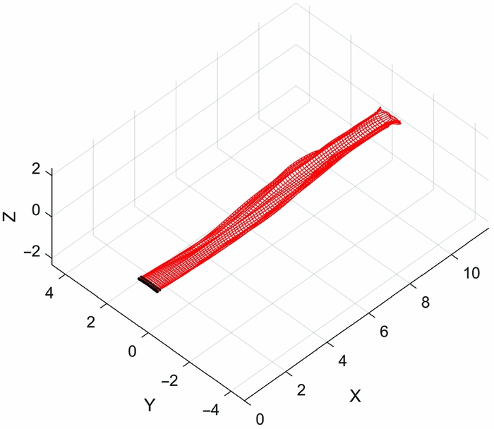
Figure 12. Wake development for flapping wing case having a reduced frequency of 0.08.
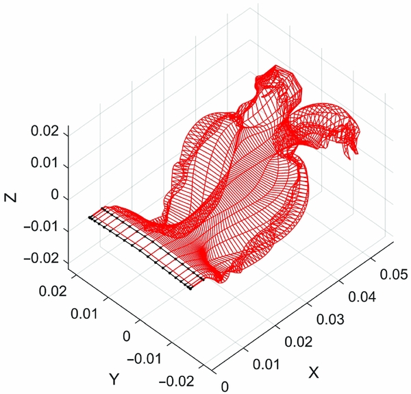
Figure 13. Wake development for flapping wing case having a reduced frequency of 1.00.
For the second step, a more sophisticated model of flapping flight combines the effects of flapping with dynamic twisting of the lifting surface. The results of the unsteady lifting-line model are compared with three-dimensional CFD results based on the Euler equations, for a relatively high airspeed value of approximately 100 m/s. The wing geometry is a rectangular planform having an aspect ratio of 8 and a NACA 0012 aerofoil section constant along the span.
The sinusoidal flapping motion is described by β = β0cos (ωt), with the amplitude β0 = 15°. The dynamic twisting is done with respect to the leading-edge line, with an amplitude that varies linearly along the span from 0° at the root section up to a maximum amplitude θ0 = 4° at the wing tips. The flapping and twisting motions are out of phase, with θ = θ0((2η)/b)sin (ωt), where η is the local span-wise coordinate and b is the wing span. The out-of-phase motions mirror the flight of birds, as this technique can avoid boundary-layer separation conditions. The flapping motion occurs at a reduced frequency k = 0.10. As for the previous analysis, the inviscid aerodynamic characteristics of the NACA 0012 aerofoil are generated using the XFOIL solver.
Comparative results are presented in Fig. 14 for the flapping-twisting wing placed at two angle-of-attack values: 0° and 4°. It can be seen that the agreement between the unsteady lifting-line model and the CFD results is very good in both cases, in terms of the amplitude and phase of the lift coefficient variation. The present results are obtained with considerable speed-up and ease compared to the CFD simulation, while not sacrificing accuracy of computations.
Figure 14. Comparison of lift coefficient results for the flapping-twisting wing at an angle-of-attack of 0° (left) and 4° (right).
3.5 Verification of wind-turbine results using experimental data
The verification of the unsteady lifting-line model is done by comparing the numerical results with experimental data gathered in the NASA Ames 80- by 120-foot wind tunnel for the NREL Phase VI rotor(Reference Hand, Simms, Fingersh, Jager, Cotrell, Schreck and Larwood43,Reference Duque, Burklund and Johnson44) . The tested turbine is a horizontal-axis two-bladed 10-m-diameter rotor operating nominally at 72 revolution per minute, the linearly tapered and twisted blades being designed based on the S809 aerofoil. A comprehensive description of the turbine geometry and of the wind-tunnel testing campaign can be found in the report by Hand et al(Reference Hand, Simms, Fingersh, Jager, Cotrell, Schreck and Larwood43). The aerofoil performance database was constructed using the data found in Ref. Reference Lindenburg45, which represent steady-state two-dimensional experimental results for a wide range of angle-of-attack values to which the three-dimensional stall delay model of Selig and Eggars was applied(Reference Lindenburg45).
The comparison is performed over a range of wind speeds between 7 and 25 m/s, with the rotor yawing angle varying between 0° and 60°. In addition to the experimental data, the comparison includes results obtained with an advanced UVLM code for the same test cases(Reference Kim, Lee and Lee46).
Figure 15 presents the variation of the rotor shaft torque as a function of the wind speed for a turbine yaw angle of 0°. It can be seen that the variation is well captured by the unsteady lifting-line model, with a good approximation of the experimental results being achieved at four of the six data points. For wind speed values of 10 and 13 m/s, the values predicted are overestimated, the prediction errors being 13% and 11%, respectively. Overall, the results obtained appear in closer agreement to the experimental data compared to the non-linear UVLM results.
Figure 15. Rotor shaft torque variation with increasing wind speed for a yaw angle of 0 degrees.
Another comparison of the calculated shaft torque values with the experimental data measured in the wind tunnel is presented in Fig. 16, for five different rotor yaw angle values between 0° and 60°, at wind speed values of 10 m/s and 15 m/s. Results demonstrate the accuracy of the unsteady lifting line in predicting rotor shaft torque values for the entire range of analysed yaw angles. Again, agreement better or comparable with the corrected UVL is achieved for the entire set of data, with the exception of the 60° yaw at 15 m/s scenario, where the obtained value is significantly higher.
Figure 16. Rotor shaft torque variation with increasing yaw angle for wind speed values of 10 m/s (left) and 15 m/s (right)
Overall, the model shows a tendency to overestimate the generated shaft torque, the error of the unsteady lifting line being on average 9–10%, while correctly capturing the shat torque variation as a function of the rotor yawing angle. Figure 17 presents the development of the wake downstream of the turbine rotor, at 0° yawing angle and a wind speed of 13 m/s, the turbine performing two full revolutions.
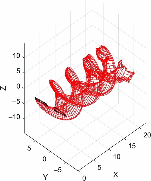
Figure 17. Wake development behind NREL Phase VI rotor during two full revolutions at no yaw and a wind speed of 13 m/s.
4.0 CONCLUSIONS
The motivation for this paper was the development of a computationally fast and accurate tool based on an unsteady non-linear lifting-line model, tool that could be applied to study of a wide range of engineering problems of interest focused on the analysis of lifting surfaces in both steady-state and unsteady flow conditions.
The method used an unsteady form of the vector form of Kutta-Joukowski theorem in order to extend its applicability to more general lifting surfaces having sweep, dihedral or other specific features such as winglets. Two-dimensional, viscous, non-linear aerodynamic characteristics of the lifting surface aerofoil were introduced through a non-linear coupling performed at each span-wise strip. The unsteady wake modelling included stable wake relaxation through a time marching scheme in a fictitious time and wake stretching and dissipation effects. Since the Jacobian matrix of the non-linear system could be determined analytically, the problem was solved using Newton's classic and efficient scheme.
The linearised form of the model provided results identical to the classical lifting-line theory for unswept lifting surfaces of moderate-to-high aspect ratio and various taper ratios. Comparisons with experimental data for low sweep wings demonstrated very good accuracy in predicting both viscous lift curve behaviour and total drag values. For swept wings, the prediction quality was very good for the lift coefficient range where the flow is fully attached on the wing surface.
Comparisons with experimental results for aerofoil in harmonic pitching and plunging motion showed very accurate prediction of the lift coefficient variation. The model was applied to the study of both low and high frequency flapping wings, and obtained results very similar to the much wider used UVLM, only offering the significant advantage of naturally introducing two-dimensional unsteady aerofoil behaviour, provided this data is available. Similar, the inviscid flow around a pitching-twisting wing was analysed with the same accuracy as inviscid CFD simulations, at only a fraction of the computational time and without requiring complex mesh generation. A study of a horizontal-axis two-bladed wind turbine was performed. Comparison with experimental results showed good accuracy in predicting the torque generated on the rotor shaft for a range of different wind speeds and rotor yaw angles.
Overall, the proposed unsteady lifting-line model showed accuracy in dealing with several different applications. The model could be applied, without any modification, for the study of multiple lifting surfaces such as wing-tail combinations, tandem flapping wings or interacting wind turbines.
APPENDIX
Consider a thin vortex sheet which at the limit can be identified with the three-dimensional surface S. At any point P on the vortex sheet, let V + and V − be the local flow velocity vectors on the two sides of S. The jump operator is defined as:
 $$\begin{equation}
\left[\kern-0.15em\left[ {{\bf V}} \right]\kern-0.15em\right] = {{{\bf V}}_ + } - {{{\bf V}}_ - }
\end{equation}$$
$$\begin{equation}
\left[\kern-0.15em\left[ {{\bf V}} \right]\kern-0.15em\right] = {{{\bf V}}_ + } - {{{\bf V}}_ - }
\end{equation}$$
If  ${\bm n}$ is the local unit vector normal to S, then the strength of the vortex sheet is by definition(Reference Wu, Ma and Zhou47) written as:
 $$\begin{equation}
{{\bf \gamma }} = {{\bf n}} \times \left[\kern-0.15em\left[ {{\bf V}} \right]\kern-0.15em\right]
\end{equation}$$
$$\begin{equation}
{{\bf \gamma }} = {{\bf n}} \times \left[\kern-0.15em\left[ {{\bf V}} \right]\kern-0.15em\right]
\end{equation}$$
Let Vγ be the velocity vector of the vortex sheet itself and  ${{\bf \bar{V}}} = \frac{1}{2}( {{{{\bf V}}_ + } + {{{\bf V}}_ - }} )$. If all vorticity is contained within the vortex sheet itself, then
  ${{{\bf V}}_{\rm{\gamma }}} = {{\bf \bar{V}}}$(Reference Wu, Ma and Zhou47). This condition is satisfied if the flow is everywhere incompressible and irrotational (potential flow), with the exception of S itself. Let ϕ be the velocity potential (thus, V = ∇ϕ) and C be a curve that connects the two sides of the sheet (at points P + and P − ). The circulation is given by:
 $$\begin{equation}
{\rm{\Gamma }} = \mathop \oint \limits_C^{} {{\bf V}} \cdot {\rm{d}}{{\bf l}} = \mathop \oint \limits_C^{} \nabla \phi \cdot {\rm{d}}{{\bf l}} = \mathop \oint \limits_C^{} \;d\phi = {\phi _ + } - {\phi _ - } = \left[\kern-0.15em\left[ \phi \right]\kern-0.15em\right]
\end{equation}$$
$$\begin{equation}
{\rm{\Gamma }} = \mathop \oint \limits_C^{} {{\bf V}} \cdot {\rm{d}}{{\bf l}} = \mathop \oint \limits_C^{} \nabla \phi \cdot {\rm{d}}{{\bf l}} = \mathop \oint \limits_C^{} \;d\phi = {\phi _ + } - {\phi _ - } = \left[\kern-0.15em\left[ \phi \right]\kern-0.15em\right]
\end{equation}$$
The vortex sheet strength (A2) becomes:
 $$\begin{equation}
{{\bf \gamma }} = {{\bf n}} \times \left[\kern-0.15em\left[ {{\bf V}} \right]\kern-0.15em\right] = {{\bf n}} \times \nabla \left[\kern-0.15em\left[ \phi \right]\kern-0.15em\right] = {{\bf n}} \times \nabla \Gamma
\end{equation}$$
$$\begin{equation}
{{\bf \gamma }} = {{\bf n}} \times \left[\kern-0.15em\left[ {{\bf V}} \right]\kern-0.15em\right] = {{\bf n}} \times \nabla \left[\kern-0.15em\left[ \phi \right]\kern-0.15em\right] = {{\bf n}} \times \nabla \Gamma
\end{equation}$$
The unsteady form of the Bernoulli equation is(Reference Katz and Plotkin9):
 $$\begin{equation}
\frac{{\partial \phi }}{{\partial t}} + \frac{1}{2}{V^2} + \frac{p}{\rho } = {\rm{const}}.
\end{equation}$$
$$\begin{equation}
\frac{{\partial \phi }}{{\partial t}} + \frac{1}{2}{V^2} + \frac{p}{\rho } = {\rm{const}}.
\end{equation}$$
Applying it to both upper and lower sides of S, and using (A1) it can be deduced for any point P:
 $$\begin{equation}
\frac{{\partial \left[\kern-0.15em\left[ \phi \right]\kern-0.15em\right]}}{{\partial t}} + \frac{1}{2}\left[\kern-0.15em\left[ {{V^2}} \right]\kern-0.15em\right] = - \frac{{\left[\kern-0.15em\left[ p \right]\kern-0.15em\right]}}{\rho }
\end{equation}$$
$$\begin{equation}
\frac{{\partial \left[\kern-0.15em\left[ \phi \right]\kern-0.15em\right]}}{{\partial t}} + \frac{1}{2}\left[\kern-0.15em\left[ {{V^2}} \right]\kern-0.15em\right] = - \frac{{\left[\kern-0.15em\left[ p \right]\kern-0.15em\right]}}{\rho }
\end{equation}$$
The dynamic pressure term can be written as:
 $$\begin{eqnarray}
&& \frac{1}{2}\left( {V_ + ^2 - V_ - ^2} \right) = \frac{1}{2}\left( {{{{\bf V}}_ + } + {{{\bf V}}_ - }} \right) \cdot \left( {{{{\bf V}}_ + } - {{{\bf V}}_ - }} \right) = {{\bf \bar{V}}} \cdot \left[\kern-0.15em\left[ {{\bf V}} \right]\kern-0.15em\right] \nonumber\\
&& \quad = {{\bf \bar{V}}} \cdot\nabla \Gamma = {{\bf \bar{V}}} \cdot \left( {{{\bf \gamma }} \times {{\bf n}}} \right) = {{\bf n}} \cdot \left( {{{\bf \bar{V}}} \times {{\bf \gamma }}} \right)
\end{eqnarray}$$
$$\begin{eqnarray}
&& \frac{1}{2}\left( {V_ + ^2 - V_ - ^2} \right) = \frac{1}{2}\left( {{{{\bf V}}_ + } + {{{\bf V}}_ - }} \right) \cdot \left( {{{{\bf V}}_ + } - {{{\bf V}}_ - }} \right) = {{\bf \bar{V}}} \cdot \left[\kern-0.15em\left[ {{\bf V}} \right]\kern-0.15em\right] \nonumber\\
&& \quad = {{\bf \bar{V}}} \cdot\nabla \Gamma = {{\bf \bar{V}}} \cdot \left( {{{\bf \gamma }} \times {{\bf n}}} \right) = {{\bf n}} \cdot \left( {{{\bf \bar{V}}} \times {{\bf \gamma }}} \right)
\end{eqnarray}$$
Consider that the vortex sheet S represents the system formed by the thin lifting surface (Sb) together with its corresponding wake (Sw), so that S = Sb∪Sw and  ${S_b}\mathop \cap \nolimits^ {S_w} = 0$. For the wake surface, the pressure on the two sides is equal, as the wake is force free p = 0. Thus, writing only for Sb and using (A7):
 $$\begin{equation}
\frac{{\partial \Gamma }}{{\partial t}} + {{\bf n}} \cdot \left( {{{\bf \bar{V}}} \times {{\bf \gamma }}} \right) = \frac{{d\Gamma }}{{dt}} = - \frac{{\left[\kern-0.15em\left[ p \right]\kern-0.15em\right]}}{\rho }
\end{equation}$$
$$\begin{equation}
\frac{{\partial \Gamma }}{{\partial t}} + {{\bf n}} \cdot \left( {{{\bf \bar{V}}} \times {{\bf \gamma }}} \right) = \frac{{d\Gamma }}{{dt}} = - \frac{{\left[\kern-0.15em\left[ p \right]\kern-0.15em\right]}}{\rho }
\end{equation}$$
The vortical impulse of a vortex sheet is defined as(Reference Saffman30,Reference Wu, Ma and Zhou47) :
 $$\begin{equation}
{{\bf I}} = \frac{1}{2}\int_V {{{\bf x}} \times {{\bf \omega }}\;dV}
\end{equation}$$
$$\begin{equation}
{{\bf I}} = \frac{1}{2}\int_V {{{\bf x}} \times {{\bf \omega }}\;dV}
\end{equation}$$
where ω = ∇ × V is the vorticity vector. Because the vorticity is only contained within the zero-thickness surface S, and using (A4), it can be written:
 $$\begin{equation}
{{\bf I}} = \frac{1}{2}\int_S {{{\bf x}} \times {{\bf \gamma }}dS = \frac{1}{2}\int_S {{\bf x} \times \left( {{\bm n} \times \nabla \Gamma } \right)dS} }
\end{equation}$$
$$\begin{equation}
{{\bf I}} = \frac{1}{2}\int_S {{{\bf x}} \times {{\bf \gamma }}dS = \frac{1}{2}\int_S {{\bf x} \times \left( {{\bm n} \times \nabla \Gamma } \right)dS} }
\end{equation}$$
The following identity is considered(Reference Wu, Ma and Zhou47):
 $$\begin{equation}
\int_S {a{{\bf n}}dS = - \frac{1}{2}} \int_S {{{\bf x}} \times \left( {{{\bf n}} \times \nabla a} \right)dS + \frac{1}{2}\int_{\partial S} {a{{\bf x}} \times {\rm{d}}{{\bf x}}} }
\end{equation}$$
$$\begin{equation}
\int_S {a{{\bf n}}dS = - \frac{1}{2}} \int_S {{{\bf x}} \times \left( {{{\bf n}} \times \nabla a} \right)dS + \frac{1}{2}\int_{\partial S} {a{{\bf x}} \times {\rm{d}}{{\bf x}}} }
\end{equation}$$
where a represents a scalar quantity defined on the surface S and ∂S is the surface boundary. Thus, if the circulation is non-zero, (A10) becomes:
 $$\begin{equation}
\frac{1}{2}\int_S {{{\bf x}} \times \left( {{{\bf n}} \times \nabla \Gamma } \right)dS = \frac{1}{2}\int_{\partial S} {\Gamma {{\bf x}} \times {\rm{d}}{{\bf x}} - } \int_S {\Gamma {{\bf n}}dS} }
\end{equation}$$
$$\begin{equation}
\frac{1}{2}\int_S {{{\bf x}} \times \left( {{{\bf n}} \times \nabla \Gamma } \right)dS = \frac{1}{2}\int_{\partial S} {\Gamma {{\bf x}} \times {\rm{d}}{{\bf x}} - } \int_S {\Gamma {{\bf n}}dS} }
\end{equation}$$
Inserting (A12) into (A10) and knowing that the circulation over the lifting surface and wake vortex sheet must drop to zero at its boundaries, it is found:
 $$\begin{equation}
{{\bf I}} = - \int_S {\Gamma {{\bf n}}dS}
\end{equation}$$
$$\begin{equation}
{{\bf I}} = - \int_S {\Gamma {{\bf n}}dS}
\end{equation}$$
Since only the lifting surface Sb generates force, the unsteady inviscid force is obtained as:
 $$\begin{equation}
{{\bf F}} = - \rho \frac{{d{{\bf I}}}}{{dt}} = \rho \frac{d}{{dt}}\int_{{S_b}} {\Gamma {{\bf n}}dS}
\end{equation}$$
$$\begin{equation}
{{\bf F}} = - \rho \frac{{d{{\bf I}}}}{{dt}} = \rho \frac{d}{{dt}}\int_{{S_b}} {\Gamma {{\bf n}}dS}
\end{equation}$$
If the lifting surface undergoes a prescribed kinematic motion such as flapping or pitching-plunging, then the orientation of the surface normal also varies in time, and we get:
 $$\begin{equation}
{{\bf F}} = \rho \int_{{S_b}} {\frac{{d\Gamma }}{{dt}}{{\bf n}}dS + \rho } \int_{{S_b}} {\Gamma \frac{d}{{dt}}\left( {{{\bf n}}dS} \right)}
\end{equation}$$
$$\begin{equation}
{{\bf F}} = \rho \int_{{S_b}} {\frac{{d\Gamma }}{{dt}}{{\bf n}}dS + \rho } \int_{{S_b}} {\Gamma \frac{d}{{dt}}\left( {{{\bf n}}dS} \right)}
\end{equation}$$
The first integral simply represents the unsteady force due to pressure difference between the two sides of the bound vortex sheet, and using (A8), it is written as:
 $$\begin{equation}
\rho \int_{{S_b}} {\frac{{d\Gamma }}{{dt}}{{\bf n}}dS = \rho } \int_{{S_b}} {\frac{{\partial \Gamma }}{{\partial t}}{{\bf n}} + \left( {{{\bf \bar{V}}} \times {{\bf \gamma }}} \right)dS = - \int_{{S_b}} {\left[\kern-0.15em\left[ p \right]\kern-0.15em\right]{{\bf n}}dS} }
\end{equation}$$
$$\begin{equation}
\rho \int_{{S_b}} {\frac{{d\Gamma }}{{dt}}{{\bf n}}dS = \rho } \int_{{S_b}} {\frac{{\partial \Gamma }}{{\partial t}}{{\bf n}} + \left( {{{\bf \bar{V}}} \times {{\bf \gamma }}} \right)dS = - \int_{{S_b}} {\left[\kern-0.15em\left[ p \right]\kern-0.15em\right]{{\bf n}}dS} }
\end{equation}$$
The second integral depends on the particular kinematics of the wing motion, and thus no general form can be given. The force becomes:
 $$\begin{equation}
{{\bf F}} = \rho \int_{{S_b}} {\frac{{\partial \Gamma }}{{\partial t}}{{\bf n}}dS + \rho } \int_{{S_b}} {\left( {{{\bf \bar{V}}} \times {{\bf \gamma }}} \right)dS + \rho } \int_{{S_b}} {\Gamma \frac{d}{{dt}}\left( {{{\bf n}}dS} \right)}
\end{equation}$$
$$\begin{equation}
{{\bf F}} = \rho \int_{{S_b}} {\frac{{\partial \Gamma }}{{\partial t}}{{\bf n}}dS + \rho } \int_{{S_b}} {\left( {{{\bf \bar{V}}} \times {{\bf \gamma }}} \right)dS + \rho } \int_{{S_b}} {\Gamma \frac{d}{{dt}}\left( {{{\bf n}}dS} \right)}
\end{equation}$$
In the context of the numerical lifting-line theory, all vorticity is further concentrated within the line vortex located at the wing quarter-chord line. Based on(Reference Saffman30), the strength of the line vortex in this case can be approximated by:
 $$\begin{equation}
{{\bf \gamma }} = \frac{1}{c}\Gamma {{\bf dl}},
\end{equation}$$
$$\begin{equation}
{{\bf \gamma }} = \frac{1}{c}\Gamma {{\bf dl}},
\end{equation}$$
where  ${{\bm dl}}$ is a local unit vector tangent to the line vortex (thus aligned with the direction of the quarter-chord line). If only a differential segment of the lifting line is considered, and the local average velocity is taken as the local flow velocity
  ${{\bm V}}$, then (A17) reduces to:
 $$\begin{equation}
{{\bf dF}} = \rho c\frac{{\partial \Gamma }}{{\partial t}}{{\bf n}} + \rho \Gamma \left( {{{\bf V}} \times {{\bf dl}}} \right) + \rho c\Gamma \frac{{d{{\bf n}}}}{{dt}}
\end{equation}$$
$$\begin{equation}
{{\bf dF}} = \rho c\frac{{\partial \Gamma }}{{\partial t}}{{\bf n}} + \rho \Gamma \left( {{{\bf V}} \times {{\bf dl}}} \right) + \rho c\Gamma \frac{{d{{\bf n}}}}{{dt}}
\end{equation}$$
ACKNOWLEDGEMENTS
The author would like to thank the reviewers for their helpful and very constructive comments, which led to a significant improvement of the quality of this paper.


