NOMENCLATURE
-
 $$\underline{W} ,\underline{Q} _{p} $$
conservative and primitive solution vectors
-
$$\underline{{\underline{\Gamma } }} $$
preconditioning matrix
-
$$\underline{{\underline{E} }} _{{({\asterisk})}} $$
elemental frames
-
$$\underline{{\underline{R} }} $$
rotational operator
-
$$\underline{{\underline{T} }} _{s} $$
relation between material and spatial angular variations
-
$$\underline{e} $$
basis vector for elemental co-ordinate
-
$$\underline{r} ,\underline{u} $$
position and displacement vectors in elemental level
-
$$\underline{{\underline{B} }} $$
transformation matrix
-
$$\underline{{\underline{E} }} $$
transformation matrix by rigid rotational operator
-
$$\underline{{\underline{P} }} $$
projector matrix
-
$$\underline{{\underline{I} }} $$
unit matrix
-
$$\underline{{\underline{N} }} _{s} $$
elemental interpolation matrix
-
$$\underline{{\underline{K} }} $$
stiffness matrix
-
$$\underline{{\underline{M} }} $$
mass matrix
-
$$\underline{{\underline{C} }} _{k} $$
gyroscopic matrix
-
$$\underline{q} ,\underline{{\dot{q}}} ,\underline{{\ddot{q}}} $$
displacement, velocity and acceleration vectors
-
$$\underline{f} ,\underline{f} _{K} ,\underline{f} _{e} $$
internal, inertial and external load vectors
-
$$\underline{a} _{m} $$
prescribed acceleration vector
- (*) G
physical quantities with respect to global frame
- (*) L
physical quantities with respect to local frame
- α,γ,β
coefficients in the HHT-α method
- h
size of the time step


1.0 INTRODUCTION
The interaction between a flexible structure and aerodynamics is an important factor when designing flapping-wing micro-aerial vehicles (MAVs). In recent decades, several experimental studies have been conducted on fluid–structure interaction (FSI) phenomena in flapping wing MAVs( Reference Ellington, Van Den Berg, Willmott and Thomas 1 – Reference Ryu, Chang and Chung 9 ). Simultaneously, numerical studies have been conducted to analyse and understand physical phenomena around the wing. Within this area of research, a variety of numerical methods have been developed ( Reference Jones, Dohring and Platzer 3 , Reference Liu, Kuykendoll, Rhew and Jones 10 - Reference Geissler and van der Wall 23 ). Reviews of the related numerical studies can be found in Refs 24 and 25.
Many researchers have attempted to understand the complex physical phenomena around such wings and have found that flexibility has a significant influence on wing performance. One related study, conducted by Heathcote et al( Reference Heathcote, Wang and Gursul 6 ), utilises three types of wings with NACA0012 cross-sections (i.e. rigid, flexible and highly flexible wings). A parametric study of the spanwise flexibility of the wing was conducted, and its influence on the wing’s aerodynamic performance was then examined. They found that the wing’s aerodynamic performance could be enhanced by moderate flexibility; otherwise, significant degradation might occur. Their experiment and relevant findings became one of the representative benchmark examples for computational studies of flapping wings. Hence, Heathcote’s experiment has been employed in numerous other computational studies( Reference Chimakurthi 14 , Reference Masarati, Morandini, Quaranta, Chandar, Roget and Sitaraman 16 - Reference Gordnier, Chimakurthi, Cesnik and Attar 19 ). In the following, some of those related to the spanwise flexibility of the wing are summarised.
Masarati et al( Reference Masarati, Morandini, Quaranta, Chandar, Roget and Sitaraman 16 ) developed an FSI analysis using an implicit coupling (tight coupling) scheme. In their analysis, a vortex lattice method was coupled with a non-linear structural analysis. This work was validated by comparison with the experimental observation conducted by Heathcote et al. Malhan et al( Reference Malhan, Lakshminarayan, Baeder and Chopra 17 ) developed an FSI framework using a Reynolds-averaged Navier–Stokes (RANS) computational fluid dynamics analysis, which was likewise validated by comparison with Heathcote’s experiment. Further, an improved FSI framework was developed by explicitly coupling with a flexible multi-body structural analysis( Reference Malhan, Baeder, Chopra and Masarati 18 ). Chimakurthi et al( Reference Chimakurthi 14 , Reference Chimakurthi, Tang, Palacios, Cesnik and Shyy 26 ) built a numerical framework to facilitate the FSI simulation of a flexible flapping wing at variable fidelity levels. A finite-volume-based Navier–Stokes fluid dynamics solver and finite-element structural solver based on a geometrically non-linear composite beam were used in their framework. The structural analysis was extended by employing a co-rotational (CR) shell element. Gordnier et al( Reference Gordnier, Chimakurthi, Cesnik and Attar 19 ) employed a computational fluid dynamics solver based on a large eddy simulation, as well as a geometrically non-linear composite beam. Then, explicit validation was conducted by accounting for the spanwise flexibility of the wing. Good agreement was obtained between the numerical results and those of Heathcote’s experiment for a few cases. The present authors developed a three-dimensional FSI framework for flapping wing MAVs by implicitly coupling a fluid dynamics solver based on the preconditioned Naver–Stokes equation with non-linear finite element analyses (planar and beam analyses) based on the CR framework ( Reference Cho, Kwak, Shin, Lee and Lee 27 , Reference Cho, Lee, Kwak, Shin and Lee 28 ). Validation was conducted by considering Heathcote’s experiment. In that study, the authors suggested some benefits of non-linear structural solvers, based on the CR framework.
One of the aims of the current paper is to develop a 3D FSI analysis by adopting a non-linear time-transient shell analysis based on the CR framework. Interest in the CR framework is increasing because of the possibility of efficient geometrically non-linear finite elements( Reference Rankin and Brogan 29 , Reference Felippa and Haugen 30 ). The present shell analysis is coupled with a 3D fluid dynamics analysis. Then, the FSI analysis is validated. Finally, a further investigation of the plunging wing will be performed to gain a comprehensive understanding of the relation between the wing performance and operating condition.
2.0 FSI FRAMEWORK
2.1 Fluid analysis
The fluid analysis is based on a 3D preconditioned Navier–Stokes equation in order to simulate the low-Mach-number flows around the plunging wings. By introducing a preconditioned pseudo-time derivative term, an integral form of the non-dimensional governing equations under a free-stream condition is expressed as follows:
 $${{\rm d} \over {{\rm d}t}}\mathop{\int}_V \underline{W} {\rm d}V{\plus}\underline{{\underline{\Gamma } }} _{a} {{\rm d} \over {{\rm d\tau }}}\mathop{\int}_V \underline{Q} _{p} {\rm d}V{\plus}\mathop{\int}_S \overleftarrow{{\underline{F} }} \cdot \underline{{\hat{n}}} {\rm d}S{\equals}\mathop{\int}_S \overleftarrow{{\underline{F} _{v} }} \cdot \underline{{\hat{n}}} {\rm d}S,$$
where
 $$\underline{W} $$
is the conservative solution vector, and
$$\underline{W} $$
is the conservative solution vector, and
 $$\underline{Q} _{p} $$
,
$$\underline{Q} _{p} $$
,
 $$\overleftarrow{{\underline{F} }} $$
and
$$\overleftarrow{{\underline{F} }} $$
and
 $$\overleftarrow{{\underline{F} _{v} }} $$
, are the primitive solution vector, inviscid flux vector and viscous flux vector, respectively. Each vectors are defined by the following relation:
$$\overleftarrow{{\underline{F} _{v} }} $$
, are the primitive solution vector, inviscid flux vector and viscous flux vector, respectively. Each vectors are defined by the following relation:
 $$\underline{W} {\equals}\left\{ {\matrix{ {\rm \rho } \cr {{\rm \rho }v_{x} } \cr {{\rm \rho }v_{y} } \cr {{\rm \rho }v_{z} } \cr {{\rm \rho }E} \cr } } \right\},\quad \overleftarrow{{\underline{F} }} {\equals}\left\{ {\matrix{ {{\rm \rho }v} \cr {{\rm \rho }vv_{x} {\plus}p\hat{i}} \cr {{\rm \rho }vv_{y} {\plus}p\hat{j}} \cr {{\rm \rho }vv_{z} {\plus}p\hat{k}} \cr {{\rm \rho }E} \cr } } \right\},\quad \overleftarrow{{\underline{F} _{v} }} {\equals}\left\{ {\matrix{ 0 \cr {{\rm \tau }_{{xi}} } \cr {{\rm \tau }_{{yi}} } \cr {{\rm \tau }_{{zi}} } \cr {{\rm \tau }_{{ij}} v_{j} {\plus}q} \cr } } \right\}$$
 $$\overleftarrow{{\underline{F} _{v} }} $$
is discretised using Roe’s approximated Riemann solver (
Reference Roe
31
) with MUSCL extrapolation (
Reference van Lear
32
). High spatial accuracy is realised by using Van Albada’s limiter. By applying the gradient theorem over an auxiliary cell, the spatial derivatives of the solution vectors are obtained at the cell interfaces. And the derivatives are employed in order to compute the viscous flux vector, which is equivalent to the second-order central difference method on a regular grid.
$$\overleftarrow{{\underline{F} _{v} }} $$
is discretised using Roe’s approximated Riemann solver (
Reference Roe
31
) with MUSCL extrapolation (
Reference van Lear
32
). High spatial accuracy is realised by using Van Albada’s limiter. By applying the gradient theorem over an auxiliary cell, the spatial derivatives of the solution vectors are obtained at the cell interfaces. And the derivatives are employed in order to compute the viscous flux vector, which is equivalent to the second-order central difference method on a regular grid.
In Equation (1),
 $$\underline{{\underline{\Gamma } }} _{a} $$
is the preconditioning matrix proposed by Weiss and Smith(
Reference Weiss and Smith
33
). By using the preconditioning matrix, it is possible to reduce the condition number of the system for low Mach number flows and to enhance the convergence of the iterative solution. And t and τ denote physical time and pseudo-time used in the time-marching procedure, respectively. For the unsteady flow analysis, the semi-discretised governing equations in fictitious time are analysed using a dual-time stepping method in conjunction with the approximate factorisation-alternate direction implicit method. The real-time derivative term is discretised by the second-order backward difference formula. After the convergence of the dual-time sub-iterations, the fictitious time term becomes zero, which ensures the second-order accurate solutions in time.
$$\underline{{\underline{\Gamma } }} _{a} $$
is the preconditioning matrix proposed by Weiss and Smith(
Reference Weiss and Smith
33
). By using the preconditioning matrix, it is possible to reduce the condition number of the system for low Mach number flows and to enhance the convergence of the iterative solution. And t and τ denote physical time and pseudo-time used in the time-marching procedure, respectively. For the unsteady flow analysis, the semi-discretised governing equations in fictitious time are analysed using a dual-time stepping method in conjunction with the approximate factorisation-alternate direction implicit method. The real-time derivative term is discretised by the second-order backward difference formula. After the convergence of the dual-time sub-iterations, the fictitious time term becomes zero, which ensures the second-order accurate solutions in time.
Details of the flow analysis are included in the literature( Reference Yoo and Lee 34 ). To consider structural deformation, a radial basis function is employed, and a geometric conservation law is utilised when computing the volume of the deforming grid.
2.2 Coupling strategy
A description of the current FSI framework is described in Refs 27 and 28. An implicit coupling approach is used to couple the structural analysis with the fluid dynamics analysis. Thus, updated coupled solutions are obtained for the same time-step at the end of the sub-iteration routine.
The current improvement of the FSI framework, compared with the authors’ previous works, is as follows. In the present fluid analysis, distributed loads are obtained by exerting pressures over the surface grids. A 3D shell analysis is used for the structural dynamics to develop improved data exchange between the fluid and structural boundaries. In the present numerical prediction, a wing stiffened by a metallic plate is employed. Thus, the following procedure for the interface is considered. First, the pressures acting on the upper and lower wing surfaces are collected. Then, those are transformed to the force vectors at grid points by integrating them with each area of the grid. And those are redefined to the force vector with respect to the intermediate plate at the centre of the wing. For the shell analysis, the relevant distributed loads are interpolated and transferred in the form of the nodal forces. A radial basis function is used for interpolation between the unmatched meshes in the fluid and structure. The present FSI framework is described in Algorithm 1.

3.0 STRUCTURAL ANALYSIS
The CR shell formulation for geometric non-linear dynamic analysis has been relatively limited because of its complex nature. To solve such limitations of the CR shell element, an approach using linearly interpolated inertial components has been used. Then, the Newmark time integration or energy-conserving algorithm is used to solve the non-linear dynamics. Zhong et al( Reference Zhong and Crisfield 35 ) compared the performance differences between the energy-conserving algorithm and Newmark-type time integration algorithms for the non-linear dynamic analysis of thin shells. However, the relevant CR formulation was not element independent, because its elastic parts adopted a specific triangular shell element. Chimakurthi et al( Reference Chimakurthi 14 ) developed a three-node CR shell dynamic analysis to consider a moving structure, which allowed the inertial terms in the shell formulation to be defined by the prescribed motion. Almeida et al( Reference Almeida and Awruch 36 ) developed an approximate energy-conserving algorithm and used it for the non-linear dynamic finite element analysis of laminated composite shells. Yang et al( Reference Yang and Xia 37 , Reference Yang and Xia 38 ) extended the generalised energy–momentum method to the CR formulations of triangular flat shell elements and to the development of a simple and practical computational method for the non-linear dynamic responses of thin shells.
In this study, an extension that considers the rigid-body motion of a flapping-wing structure is conducted by including the non-linear inertial terms defined in accordance with the CR framework for a three-node triangular shell. Thus, the existing co-ordinates in the CR framework are considered to be a dynamic frame obeying the moving structure. This approach is based on that suggested by the previous studies( Reference Yang and Xia 38 – Reference Le, Battini and Hjiaj 41 ). The relevant description of the CR framework is presented in the following subsection.
3.1 CR framework
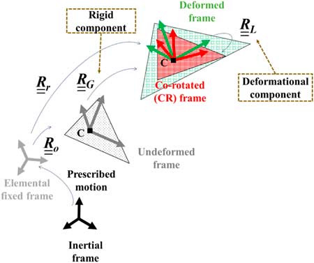
The CR formulation can be established by tracking a co-ordinate-based elemental motion.
The CR co-ordinate is an additional intermediate configuration between the undeformed and deformed frames. The local system can be defined between the CR and local co-ordinates. Figure 1 shows the co-ordinates and related transformations obeying the elemental kinematics for a three-node shell element. Beginning with the elemental fixed frame
 $$\underline{{\underline{E} }} _{I} $$
, the rotational matrix
$$\underline{{\underline{E} }} _{I} $$
, the rotational matrix
 $$\underline{{\underline{R} }} _{o} $$
can be defined by tracking the elemental initial state. The rotational matrix
$$\underline{{\underline{R} }} _{o} $$
can be defined by tracking the elemental initial state. The rotational matrix
 $$\underline{{\underline{R} }} _{G} $$
can be defined by elemental rotational displacement referring to an undeformed configuration
$$\underline{{\underline{R} }} _{G} $$
can be defined by elemental rotational displacement referring to an undeformed configuration
 $$\underline{{\underline{E} }} _{G} $$
. The complete rotation can be decomposed into rigid body rotation referring to the CR frame
$$\underline{{\underline{E} }} _{G} $$
. The complete rotation can be decomposed into rigid body rotation referring to the CR frame
 $$\underline{{\underline{E} }} _{C} $$
and elastic deformational rotation referring to a deformed configuration
$$\underline{{\underline{E} }} _{C} $$
and elastic deformational rotation referring to a deformed configuration
 $$\underline{{\underline{E} }} _{L} $$
. The origin of each co-ordinate is taken at the centroid. Each transformation can be accomplished by rotational operators
$$\underline{{\underline{E} }} _{L} $$
. The origin of each co-ordinate is taken at the centroid. Each transformation can be accomplished by rotational operators
 $$\underline{{\underline{R} }} _{G} $$
,
$$\underline{{\underline{R} }} _{G} $$
,
 $$\underline{{\underline{R} }} _{r} $$
and
$$\underline{{\underline{R} }} _{r} $$
and
 $$\underline{{\underline{R} }} _{L} $$
, which are composed of the global, rigid-body and local rotations θ
G
, θ
r
and θ
L
, respectively. Here, the local rotational variables are obtained by multiplying the operators:
$$\underline{{\underline{R} }} _{L} $$
, which are composed of the global, rigid-body and local rotations θ
G
, θ
r
and θ
L
, respectively. Here, the local rotational variables are obtained by multiplying the operators:
 $$\underline{{\underline{R} }} _{L} {\equals}\underline{{\underline{R} }} _{r}^{T} \underline{{\underline{R} }} _{G} \underline{{\underline{R} }} _{o} $$
.
$$\underline{{\underline{R} }} _{L} {\equals}\underline{{\underline{R} }} _{r}^{T} \underline{{\underline{R} }} _{G} \underline{{\underline{R} }} _{o} $$
.

Figure 1 Co-ordinates and elemental kinematics in the CR formulation for 3-node shell.
It is noted that the origin of the co-ordinate is different from that used in the previous FSI study( Reference Chimakurthi 14 ) and the present co-ordinates follows Battini’s approach( Reference Battini 40 ). Thus, it becomes possible to obtain stable solution without the effect of sequence in elemental nodes. Details of the advantages regarding the present approach are described in Battini( Reference Battini 40 ).
In the present formulation, the rotational operator can be defined by Rodrigues’ formula:
 $$\underline{{\underline{R} }} {\equals}\underline{{\underline{I} }} {\plus}{{\sin {\rm \rtheta }} \over {\rm \rtheta }}\underline{{{\tilde {\rtheta }}}} {\plus}{{1{\minus}\cos {\rm \rtheta }} \over {{\rm \rtheta }^{2} }}\underline{{{\tilde{\rtheta }}}} ^{2} $$
where a tilde denotes the skew-symmetric matrix. The spatial variation can be described using the following relation:
 $${\rm \delta }\underline{{\tilde{\phi }}} {\equals}\underline{{\underline{T} }} _{s} (\underline{{\rm \rtheta }} ){\rm \delta }\underline{{{\tilde{\psi }}}} $$
where
 $${\rm \delta }\underline{{{\tilde{\psi }}}} $$
and
$${\rm \delta }\underline{{{\tilde{\psi }}}} $$
and
 $${\rm \delta }\underline{{\tilde{\phi }}} $$
denote material and spatial angular variations (i.e. infinitesimal rotations superimposed onto the rotational matrix), respectively. The relevant variations obey the relation
$${\rm \delta }\underline{{\tilde{\phi }}} $$
denote material and spatial angular variations (i.e. infinitesimal rotations superimposed onto the rotational matrix), respectively. The relevant variations obey the relation
 $${\rm \delta }\underline{{\underline{R} }} {\equals}({\rm \delta }\underline{{\tilde{\phi }}} )\underline{{\underline{R} }} {\equals}\underline{{\underline{R} }} ({\rm \delta }\underline{{{\rm \tilde{\psi }}}} )$$
. Further,
$${\rm \delta }\underline{{\underline{R} }} {\equals}({\rm \delta }\underline{{\tilde{\phi }}} )\underline{{\underline{R} }} {\equals}\underline{{\underline{R} }} ({\rm \delta }\underline{{{\rm \tilde{\psi }}}} )$$
. Further,
 $$\underline{{\underline{T} }} _{s} $$
is expressed as
$$\underline{{\underline{T} }} _{s} $$
is expressed as
 $$\underline{{\underline{T} }} _{s} (\underline{{\rm \rtheta }} ){\equals}\underline{{\underline{I} }} {\plus}{{1{\minus}\cos {\rm \rtheta }} \over {{\rm \rtheta }^{2} }}\underline{{{\tilde{\rtheta }}}} {\plus}{{{\rm \rtheta }{\minus}\sin {\rm \rtheta }} \over {{\rm \rtheta }^{3} }}\underline{{{\tilde{\rtheta }}}} ^{2} .$$
The local displacement
 $$\underline{u} _{L}^{i} $$
of the element is given by the following equation:
$$\underline{u} _{L}^{i} $$
of the element is given by the following equation:
 $$\underline{u} _{L}^{i} {\equals}\underline{{\underline{R} }} _{r}^{T} \left\{ {\underline{r} ^{i} {\plus}\underline{u} _{G}^{i} {\minus}\underline{r} ^{c} {\minus}\underline{u} _{G}^{c} } \right\}{\minus}\underline{{\underline{R} }} _{o} \left\{ {\underline{r} ^{i} {\minus}\underline{r} ^{c} } \right\}$$
where the superscript i denotes an arbitrary node of the element. The geometric and rigid body rotations consisting of
 $$\underline{{\underline{R} }} _{o} $$
and
$$\underline{{\underline{R} }} _{o} $$
and
 $$\underline{{\underline{R} }} _{r} $$
are defined with respect to the elemental reference frame.
$$\underline{{\underline{R} }} _{r} $$
are defined with respect to the elemental reference frame.
Let
 $$\underline{e} _{C} $$
denote the orthonormal basis vectors on the element. Then, the orthogonal matrix defining the rigid rotations is simply given by
$$\underline{e} _{C} $$
denote the orthonormal basis vectors on the element. Then, the orthogonal matrix defining the rigid rotations is simply given by
 $$\matrix{ {\underline{{\underline{R} }} _{r} {\equals}[\underline{e} _{{C,1}} } & {\underline{e} _{{C,2}} } & {\underline{e} _{{C,3}} ].} \cr } $$
The first co-ordinate axis referring to the CR frame
 $$\underline{e} _{{C,1}} $$
is selected as the basis of the vector parallel to the side connected between nodes 1 and 2:
$$\underline{e} _{{C,1}} $$
is selected as the basis of the vector parallel to the side connected between nodes 1 and 2:
 $$\underline{e} _{{C,1}} {\equals}{{\underline{r} _{G}^{2} {\plus}\underline{u} _{G}^{2} {\minus}\underline{r} _{G}^{1} {\minus}\underline{u} _{G}^{1} } \over {\parallel\underline{r} _{G}^{2} {\plus}\underline{u} _{G}^{2} {\minus}\underline{r} _{G}^{1} {\minus}\underline{u} _{G}^{1} \parallel}}$$
Using an auxiliary vector,
 $$\underline{r} _{{3c}} {\equals}\underline{r} _{G}^{3} {\plus}\underline{u} _{G}^{3} {\minus}\underline{r} _{G}^{c} {\minus}\underline{u} _{G}^{c} $$
, the third co-ordinate axis,
$$\underline{r} _{{3c}} {\equals}\underline{r} _{G}^{3} {\plus}\underline{u} _{G}^{3} {\minus}\underline{r} _{G}^{c} {\minus}\underline{u} _{G}^{c} $$
, the third co-ordinate axis,
 $$\underline{e} _{{C,3}} $$
, is assumed to be orthogonal to the elemental plane:
$$\underline{e} _{{C,3}} $$
, is assumed to be orthogonal to the elemental plane:
 $$\underline{e} _{{C,3}} {\equals}{{\underline{e} _{{C,1}} {\times}\underline{r} _{{3c}} } \over {\parallel\underline{e} _{{C,1}} {\times}\underline{r} _{{3c}} \parallel}}$$
The second co-ordinate axis,
 $$\underline{e} _{{C,2}} $$
, is then obtained by the following expression:
$$\underline{e} _{{C,2}} $$
, is then obtained by the following expression:
 $$\underline{e} _{{C,3}} {\times}\underline{e} _{{C,1}} $$
.
$$\underline{e} _{{C,3}} {\times}\underline{e} _{{C,1}} $$
.
Thus, it is possible to establish the rotational operators,
 $$\underline{{\underline{R} }} _{o} $$
and
$$\underline{{\underline{R} }} _{o} $$
and
 $$\underline{{\underline{R} }} _{r} $$
. By obeying the elemental kinematics, the stiffness matrix and internal load vector for the triangular shells can be derived. The virtual energy can be defined by equating the local/global internal load vectors and the variation of the corresponding nodal displacement vectors:
$$\underline{{\underline{R} }} _{r} $$
. By obeying the elemental kinematics, the stiffness matrix and internal load vector for the triangular shells can be derived. The virtual energy can be defined by equating the local/global internal load vectors and the variation of the corresponding nodal displacement vectors:
 $$V{\equals}{\rm \delta }\underline{q} _{L}^{T} \underline{f} _{L} {\equals}{\rm \delta }\underline{q} _{G}^{T} \underline{f} _{G} $$
By equating the relationship between the local and global internal load vectors, Equation (10), the local internal load vector is defined as follows:
 $$\underline{f} _{L} {\equals}\underline{{\underline{B} }} \underline{f} _{G} $$
The global tangent stiffness matrix is defined by taking the variations of Equations (11):
 $$\underline{{\underline{K} }} _{G} {\equals}\underline{{\underline{B} }} ^{T} \underline{{\underline{K} }} _{L} \underline{{\underline{B} }} {\plus}{{\partial (\underline{{\underline{B} }} ^{T} \underline{f} _{L} )} \over {\partial \underline{q} _{G} }}{\rfloor}_{{\underline{f} _{L} }} $$
For the local system,
 $$\underline{{\underline{K} }} _{L} $$
, the OPT-DKT facet shell element(
Reference Khosravi, Ganesan and Sedaghati
42
) is used in the current shell analysis. The transformation matrix
$$\underline{{\underline{K} }} _{L} $$
, the OPT-DKT facet shell element(
Reference Khosravi, Ganesan and Sedaghati
42
) is used in the current shell analysis. The transformation matrix
 $$\underline{{\underline{B} }} $$
can be defined by introducing the rigid body and deformational components:
$$\underline{{\underline{B} }} $$
can be defined by introducing the rigid body and deformational components:
 $$\underline{{\underline{B} }} {\equals}\underline{{\underline{E} }} \underline{{\underline{P} }} ^{T} $$
where
 $$\underline{{\underline{E} }} $$
is determined using the rotational operator
$$\underline{{\underline{E} }} $$
is determined using the rotational operator
 $$\underline{{\underline{R} }} _{r} $$
, and
$$\underline{{\underline{R} }} _{r} $$
, and
 $$\underline{{\underline{P} }} $$
is the projector matrix, considering the deformational components. Details of the derivations related to the stiffness matrix and internal load vector are presented in Refs 39 and 43.
$$\underline{{\underline{P} }} $$
is the projector matrix, considering the deformational components. Details of the derivations related to the stiffness matrix and internal load vector are presented in Refs 39 and 43.
3.2 Inertial terms based on CR framework
The derivation of the inertial force vector and elemental inertial matrices, i.e. the mass and gyroscopic matrices, is presented. The relevant formulation is based on Ref. 41. The kinetic energy of the element is expressed by considering the velocity vector:
 $${\cal K}{\equals}{1 \over 2}\mathop{\int}_\Omega {\rm \rho }\underline{{\dot{q}}} ^{T} \underline{{\dot{q}}} {\rm d\Omega }$$
where
 $$\underline{{\dot{q}}} $$
denotes the velocity vector. The kinetic energy can be re-expressed using the translational and rotational components:
$$\underline{{\dot{q}}} $$
denotes the velocity vector. The kinetic energy can be re-expressed using the translational and rotational components:
 $${\cal K}{\equals}{1 \over 2}\mathop{\int}_\Omega \underline{{\dot{u}}} ^{T} m_{\rho } \underline{{\dot{u}}} {\plus}\underline{{{\dot{\rtheta }}}} ^{T} \underline{{\underline{I} }} _{{\rm \rho }} \underline{{{\dot{\rtheta }}}} {\rm d\Omega }$$
where m
ρ
=ρ
t, and
 $$\underline{{\underline{I} }} _{{\rm \rho }} $$
is the spatial dyadic tensor given by
$$\underline{{\underline{I} }} _{{\rm \rho }} $$
is the spatial dyadic tensor given by
 $${\rm diag}\left( {{{{\rm \rho }t^{3} } \over {12}},{{{\rm \rho }t^{3} } \over {12}},0} \right)$$
.
$${\rm diag}\left( {{{{\rm \rho }t^{3} } \over {12}},{{{\rm \rho }t^{3} } \over {12}},0} \right)$$
.
The kinetic energy variation can be expressed in terms of the material velocity and acceleration:
 $${\rm \delta }{\cal K}{\equals}\mathop{\int}_\Omega {\rm \delta }\underline{u} ^{T} m_{\rho } \underline{{\ddot{u}}} {\plus}{\rm \delta }\underline{{\rm \rtheta }} [\underline{{\underline{I} }} _{{\rm \rho }} \underline{{{\ddot{\rtheta }}}} {\plus}\underline{{{\tilde{\dot{\rtheta }}}}} \underline{{\underline{I} }} _{{\rm \rho }} \underline{{{\dot{\rtheta }}}} ]{\rm d\Omega }.$$
The material velocity and acceleration with respect to the local co-ordinate can be defined using elemental kinematics:
 $${\rm \delta }\underline{{\dot{q}}} _{L} {\equals}\underline{{\underline{E} }} ^{T} {\rm \delta }\underline{{\dot{q}}} _{G} $$
 $${\rm \delta }\underline{{\ddot{q}}} _{L} {\equals}\underline{{\underline{E} }} ^{T} {\rm \delta }\underline{{\ddot{q}}} _{G} .$$
Consequently, by employing matrix
 $$\underline{{\underline{N} }} _{s} $$
, which is composed of element nodal shape functions, the nodal quantities can be re-expressed in terms of those functions at the element level:
$$\underline{{\underline{N} }} _{s} $$
, which is composed of element nodal shape functions, the nodal quantities can be re-expressed in terms of those functions at the element level:
 $$\underline{q} _{L} {\equals}\underline{{\underline{N} }} _{s} \underline{q} _{L} {\equals}\left\{ {\underline{u} ^{T} \quad \underline{{\rm \rtheta }} ^{T} } \right\}^{T} .$$
The inertial load vector is derived from the relation
 $${\rm \delta }{\cal K}{\equals}\underline{f} _{{k,G}}^{T} \underline{q} _{G} $$
. Recalling the relation in Equation (11), the expression of the inertial load vector is obtained as follows:
$${\rm \delta }{\cal K}{\equals}\underline{f} _{{k,G}}^{T} \underline{q} _{G} $$
. Recalling the relation in Equation (11), the expression of the inertial load vector is obtained as follows:
 $$\underline{f} _{{k,G}} {\equals}\left\{ {\underline{f} _{{k,G}}^{1} ^{T} \quad \underline{f} _{{k,G}}^{2} ^{T} \quad \underline{f} _{{k,G}}^{3} ^{T} } \right\}^{T} $$
 $$\underline{f} _{{k,G}}^{i} {\equals}\underline{{\underline{E} }} \underline{f} _{{k,L}}^{i} {\equals}\underline{{\underline{E} }} \left\{ {\matrix{ {\mathop{\int}_{\Omega _{e} } N^{i} m_{{\rm \rho }} \underline{{\ddot{u}}} {\rm d\Omega }_{e} } & {} \cr {\mathop{\int}_{\Omega _{e} } N^{i} (\underline{{\underline{I} }} _{{\rm \rho }} \underline{{{\ddot{\rtheta }}}} {\plus}\underline{{{\tilde{\dot{\rtheta }}}}} \underline{{\underline{I} }} _{{\rm \rho }} \underline{{\rm \rtheta }} ){\rm d\Omega }_{e} } & {} \cr } } \right\},\quad i{\equals}1,2,3$$
Linearisation of the variation form of the kinetic energy yields the mass and gyroscopic matrices:
 $$\underline{{\underline{M} }} _{G}^{{i,j}} {\equals}\underline{{\underline{E} }} ^{T} \left[ {\matrix{ {\left( {\mathop{\int}_{\Omega _{e} } N^{i} N^{j} m_{{\rm \rho }} {\rm d\Omega }_{e} } \right)\underline{{\underline{I} }} _{3} } & {\underline{0} _{3} } \cr {\underline{0} _{3} } & {\mathop{\int}_{\Omega _{e} } N^{i} N^{j} \underline{{\underline{I} }} _{\rho } \underline{{\underline{T} }} _{s}^{{{\minus}1}} (\underline{{\rm \rtheta }} ){\rm d\Omega }_{e} } \cr } } \right]\underline{{\underline{E} }} $$
 $$\underline{{\underline{C} }} _{{k,G}}^{{i,j}} {\equals}\underline{{\underline{E} }} ^{T} \left[ {\matrix{ {\underline{{\underline{0} }} _{3} } & {\underline{0} _{3} } \cr {\underline{0} _{3} } & {\mathop{\int}_{\Omega _{e} } N^{i} N^{j} (\tilde \dot \underline {\rtheta } \underline{{\underline{I} }} _{{\rm \rho }} {\minus}\widetilde{{\underline{{\underline{I} }} _{{\rm \rho }} \dot \underline{{\rm \rtheta }} }})\underline{{\underline{T} }} _{s}^{{{\minus}1}} (\underline{{\rm \rtheta }} ){\rm d\Omega }_{e} } \cr } } \right]\underline{{\underline{E} }} $$
3.3 Governing equation for time-transient analysis
To solve the non-linear dynamic equation, the Hilbert Hughes Taylor (HHT)-α method is used. The resulting algorithm is of the predictor-corrector type, similar to that used in an earlier study( Reference Crisfield 44 , Reference Le, Battini and Hjiaj 45 ). In non-linear time-transient structural analyses, the displacements, velocities and accelerations are obtained iteratively at each time-step, i.e. by a Newton–Raphson scheme.
Linearisation of the inertial load vector is required to obtain the tangent inertial matrix. The final form of the tangent dynamic stiffness matrix is expressed as
 $$\underline{{\underline{K} }} _{{Dyn,G}}^{{\rm \alpha }} {\equals}{1 \over {{\rm \beta }h^{2} }}\underline{{\underline{M} }} _{G} {\plus}{{\rm \gamma } \over {{\rm \beta }h}}\underline{{\underline{C} }} _{{k,G}} {\plus}\underline{{\underline{K} }} _{G} $$
where
 $$\underline{{\underline{M} }} _{G} $$
,
$$\underline{{\underline{M} }} _{G} $$
,
 $$\underline{{\underline{C} }} _{{k,G}} $$
and
$$\underline{{\underline{C} }} _{{k,G}} $$
and
 $$\underline{{\underline{K} }} _{G} $$
respectively denote the mass, and gyroscopic and stiffness matrices, with respect to the global co-ordinate.
$$\underline{{\underline{K} }} _{G} $$
respectively denote the mass, and gyroscopic and stiffness matrices, with respect to the global co-ordinate.
The governing equation of a moving structure can be expressed as
 $$(1{\plus}{\rm \alpha })\underline{f} _{e}^{{n{\plus}1}} {\minus}(1{\plus}{\rm \alpha })\underline{f} _{G}^{{n{\plus}1}} {\minus}\underline{f} _{{Km,G}}^{{n{\plus}1}} {\plus}{\rm \alpha }\left( {\underline{f} _{G}^{{,n}} {\minus}\underline{f} _{e}^{n} } \right){\equals}\underline{0} $$
where
 $$\underline{f} _{e} $$
,
$$\underline{f} _{e} $$
,
 $$\underline{f} _{G} $$
and
$$\underline{f} _{G} $$
and
 $$\underline{f} _{{Km,G}} $$
denote the external, internal and inertial force vectors, respectively. The prescribed motion is now considered to be the relevant acceleration of the motion:
$$\underline{f} _{{Km,G}} $$
denote the external, internal and inertial force vectors, respectively. The prescribed motion is now considered to be the relevant acceleration of the motion:
 $$\underline{f} _{{Km,G}} {\equals}\underline{f} _{{k,G}} {\minus}\underline{{\underline{M} }} _{G} \underline{a} _{m} $$
where
 $$\underline{a} _{m} $$
denotes the acceleration of the motion. At the element level,
$$\underline{a} _{m} $$
denotes the acceleration of the motion. At the element level,
 $$\underline{a} _{m} $$
can be expressed as follows:
$$\underline{a} _{m} $$
can be expressed as follows:
 $$\underline{a} _{m} {\equals}\left\{ {\matrix{ {\underline{a} _{{m,u}}^{T} } & {\underline{a} _{{m,{\rm \rtheta }}}^{T} } \cr } } \right\}^{T} $$
where
 $$\underline{a} _{{m,u}} $$
and
$$\underline{a} _{{m,u}} $$
and
 $$\underline{a} _{{m,{\rm \rtheta }}} $$
are defined by the relevant acceleration of the translational (
$$\underline{a} _{{m,{\rm \rtheta }}} $$
are defined by the relevant acceleration of the translational (
 $$\underline{{\ddot{u}}} _{p} $$
) and rotational (
$$\underline{{\ddot{u}}} _{p} $$
) and rotational (
 $$\underline{{{\ddot{\rtheta }}}} _{p} $$
) motions, respectively:
$$\underline{{{\ddot{\rtheta }}}} _{p} $$
) motions, respectively:
 $$\underline{a} _{{m,u}} {\equals}\underline{{{\tilde{\ddot{\rtheta }}}}} _{p} \underline{X} _{p} {\plus}\underline{{\ddot{u}}} _{p} $$
 $$\underline{a} _{{m,\rtheta }} {\equals}\underline{{{\ddot{\rtheta }}}} _{p} $$
In the following sections, the FSI analysis is validated using the results of Heathcote’s experiment.
4.0 VALIDATION OF PRESENT FSI ANALYSIS
4.1 Description of experiment
The present FSI framework is validated by comparison with the results observed in the experiment conducted by Heathcote et al( Reference Heathcote, Wang and Gursul 6 ). Heathcote’s experiment considered rectangular cantilevered wings with different degrees of flexibility. The three types of wings (rigid, flexible and highly flexible) possessed different degrees of spanwise flexibility under a prescribed plunging motion.
Table 1 lists the operating conditions used in the present analysis. The reduced frequency k
G
was varied from 0 to 1.82. k
G
is defined by
 $$k_{G} {\equals}{{\pi f_{m} c} \over {U_{\infty} }}$$
, accounting for plunging frequency f
m
, chord length c and free-stream velocity U
∞. The rigid, flexible and highly flexible wings were designed to be stiff, intermediately flexible and extremely flexible, respectively. In this study, the flexible and highly flexible wings are analysed in the present FSI analysis. The flexible and highly flexible wings were fabricated using polydimethylsiloxane rubber (PDMS) cast in an NACA0012 mold. The flexible wing was additionally reinforced using s 1-mm stainless steel plate, whereas 1-mm aluminium plate was used for the highly flexible wing. Cross-sections of the relevant configurations are shown in Fig. 2.
$$k_{G} {\equals}{{\pi f_{m} c} \over {U_{\infty} }}$$
, accounting for plunging frequency f
m
, chord length c and free-stream velocity U
∞. The rigid, flexible and highly flexible wings were designed to be stiff, intermediately flexible and extremely flexible, respectively. In this study, the flexible and highly flexible wings are analysed in the present FSI analysis. The flexible and highly flexible wings were fabricated using polydimethylsiloxane rubber (PDMS) cast in an NACA0012 mold. The flexible wing was additionally reinforced using s 1-mm stainless steel plate, whereas 1-mm aluminium plate was used for the highly flexible wing. Cross-sections of the relevant configurations are shown in Fig. 2.
Table 1 Operating conditions


Figure 2 Cross-section of the flexible and highly flexible wings( Reference Heathcote, Wang and Gursul 6 ).
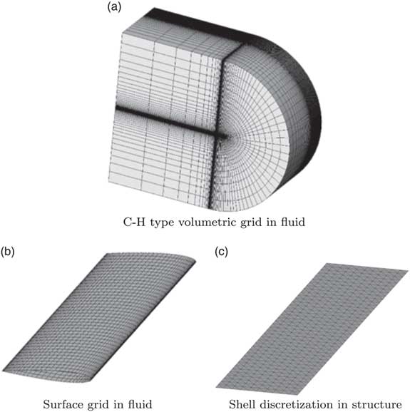
After the grid sensitivity analysis is completed, 389,400 grid cells and 29,000 surface boundary nodes are chosen in the current fluid analysis, and 936 elements are employed in the present shell analysis. A complete 3D wing configuration is considered in the fluid analysis, although the 3D configuration is reduced to a 2D plate for the shell analysis. The detailed discretisation in fluid and structural analyses is shown in Fig. 3, and the material properties of the flexible and highly flexible wings are provided in Table 2.

Figure 3 Discretisation information in the present FSI analysis.
Table 2 Structural properties used in the previous studies( Reference Chimakurthi 14 , Reference Gordnier, Chimakurthi, Cesnik and Attar 19 )

4.2 Validation with previous experimental results (k G =1.82)
This subsection compares the present results with those obtained from previous studies and experiments. Mainly, the flexible and highly flexible wings are considered. First, the previous numerical and experimental results are compared with the present result when k G is equal to 1.82. Figure 4 shows a comparison of the thrust coefficient histories. The average values for the thrust coefficient are then compared, and a summary of the relevant values is presented in Table 3

Figure 4 Comparison of the thrust coefficient history.
Table 3 Summary of averaged values of the thrust coefficient history

. The differences are obtained by subtracting the relevant physical quantities (Table 3).
For the flexible wing, the present thrust coefficient history shows good agreement with that observed in the experiment (Fig. 4). Further, the present prediction regarding the highly flexible wing shows a trend similar to that predicted by Gordnier et al using a higher-order fluid dynamic analysis (Fig. 4). However, the high-frequency response observed in the experiment was not captured in either prediction. In neither the present nor previous studies( Reference Chimakurthi 14 , Reference Gordnier, Chimakurthi, Cesnik and Attar 19 ), physical reason regarding the high-frequency response is obtained. Extensive investigation of such FSI phenomena in the highly flexible wing will still be required.
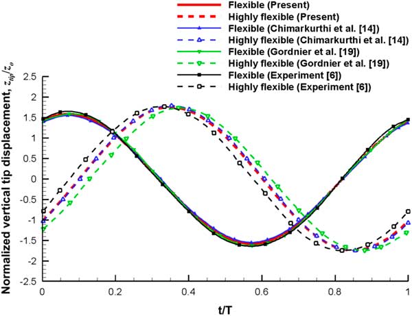
The wing tip displacement history is illustrated in Fig. 5. The tip displacement z tip is normalised by the amplitude of the plunge motion z o . For the flexible wing, the present prediction exhibits a phase difference compared with the previous numerical and experimental results. However, the present result still correlates reasonably with the experimental results. Regarding the structural flexibility, a phase variation in the tip history is induced as a result of inertial and aerodynamic forces, which becomes more significant for the highly flexible wing. The relative differences in the peak-to-peak values and degrees of phase variation in the tip displacement history are summarised in Table 4.

Figure 5 Comparison of the wing tip displacement history.
Table 4 Summary of peak-to-peak value and phase difference in the wing tip displacement history

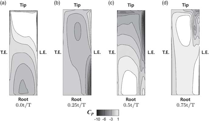
Then, the pressure coefficient C P on the wing surface is presented in order to evaluate the influence of the wing flexibility in detail. The relevant comparison is conducted in situations with 0.0 t/T, 0.25 t/T, 0.5 t/T and 0.75 t/T. The relevant comparisons between the present results for the flexible and highly flexible wings are presented in Figs 6 and 7, respectively. Figure 6 shows the pressure distribution of the flexible wing, and it is found that the pressure distribution is uniform in the spanwise direction in all situations. For the highly flexible wing, the variation of the pressure distribution in the spanwise direction is significant (Fig. 7). This phenomenon is due to the phase-lagging motion of the wing tip. Thus, lower and higher pressure regions exist simultaneously around the leading edge. Specifically, the difference in the pressure distribution along the spanwise direction is significant for 0.0 t/T and 0.5 t/T. As a result, degradation of the thrust coefficient is shown in the highly flexible wing. This phenomenon was also predicted by the previous studies, and it was found that an intermediate flexibility may be beneficial for increasing the thrust.

Figure 6 Pressure coefficient, C P, on the surface of the flexible wing (k G=1.82).

Figure 7 Pressure coefficient, C P, on the surface of the highly flexible wing (k G=1.82).
5.0 EXTENSIVE PREDICTION FOR PLUNGING WING (k G =0-4.8)
In the previous studies, a range of 0-1.82 was selected for k
G
, and it is further extended to a range of 0-4.8. For natural flyers, the propulsive efficiency is high over a narrow Strouhal number range, which is generally 0.2-0.4. The Strouhal number describes the oscillating flow mechanism, and it can be given as
 $$S_{t} {\equals}{{2k_{G} z_{o} } \over {\pi c}}$$
. Thus, an extended k
G
range for S
t
can be considered to be 0–0.53. First, the averaged C
T
, and normalised amplitude and phase shift of the wing tip displacement, will be compared to the experimental results with respect to the reduced frequency. Then, the power coefficient C
P
will be analysed.
$$S_{t} {\equals}{{2k_{G} z_{o} } \over {\pi c}}$$
. Thus, an extended k
G
range for S
t
can be considered to be 0–0.53. First, the averaged C
T
, and normalised amplitude and phase shift of the wing tip displacement, will be compared to the experimental results with respect to the reduced frequency. Then, the power coefficient C
P
will be analysed.
Figure 8 shows a comparison of the averaged C T with respect to the reduced frequency. The present prediction is compared to the experimental results (k G =0–1.82), and it is found that the present results show good correlations for both the flexible and highly flexible wings. Regarding the highly flexible wing, due to the significant bending motion of the wing, degradation in the increasing rate of the averaged C T (degradation in the slope of the k G -averaged C T graph) is captured in k G range of 0–1.82. However, the increasing rate is enlarged when k G is larger than 1.82. On the other hand, the increasing rate of the averaged C T for the flexible wing is decreased when k G is larger than 2.3.

Figure 8 Comparison of the averaged C T with respect to k G (k G =0–4.8).
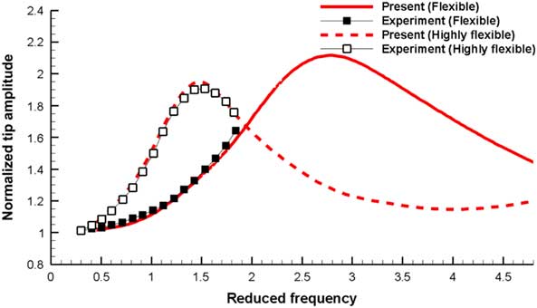
Next, the normalised amplitude of the wing tip displacement with respect to k G is analysed. The present results are also compared to the experimental results. The relevant comparison is shown in Fig. 9. It is also found that the present results show good correlations with the experimental results for both the flexible and highly flexible wings when k G is 0–1.82. When k G is greater than 1.5, the tip amplitude decreases for the highly flexible wing. This situation is also found for the flexible wing, when k G is greater than 2.8. On the other hand, the drastic decrease in the wing tip amplitude for the highly flexible wing is stabilised when k G is further increased, and the relevant normalised value is approximately 1.2.

Figure 9 Comparison of the wing tip amplitude with respect to k G (k G =0–4.8).
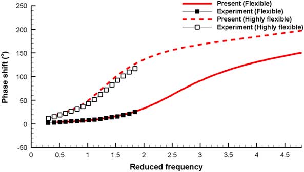
A comparison of the phase shift values for the wing tip displacement is shown in Fig. 10. The present results show good agreement with the experimental results for both the flexible and highly flexible wings, when k G is 0–1.82. A significant phase shift is predicted for the highly flexible wing compared to that for the flexible wing. When k G is greater than 3.8, the phase shift becomes larger than 180°. Regarding the flexible wing, the increase in the phase shift is significant when k G is near 2.3.

Figure 10 Comparison of phase shift in wing tip displacement with respect to k G (k G =0-4.8).
Finally, the power coefficient of each wing is analysed. The relevant physical value is obtained by
 $${{F_{z} v_{{{\rm root}}} } \over {0.5{\rm \rho }U_{\infty}^{3} c}}$$
. Here, F
z
is the aerodynamic load in the vertical direction, and v
root is the velocity of the wing root. A comparison of the averaged power coefficients is shown in Fig. 11. The power required by the flexible wing is larger than that of the highly flexible wing. In addition, the power coefficient trend with respect to k
G
is similar to that of the averaged C
T
.
$${{F_{z} v_{{{\rm root}}} } \over {0.5{\rm \rho }U_{\infty}^{3} c}}$$
. Here, F
z
is the aerodynamic load in the vertical direction, and v
root is the velocity of the wing root. A comparison of the averaged power coefficients is shown in Fig. 11. The power required by the flexible wing is larger than that of the highly flexible wing. In addition, the power coefficient trend with respect to k
G
is similar to that of the averaged C
T
.
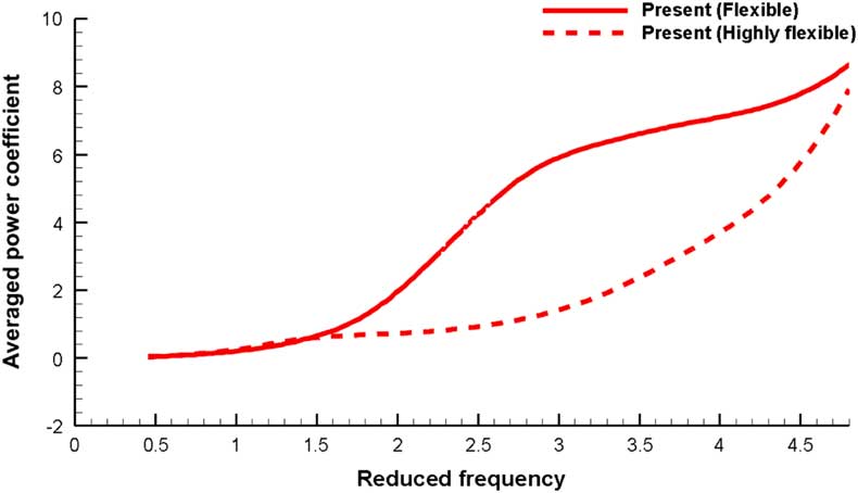
Figure 11 Comparison of the averaged power coefficient with respect to k G (k G =0-4.8).
The present analysis is further validated and extensive predictions are performed using four physical quantities with respect to k G . The degradation of the increasing rate of the thrust coefficient is predicted for the flexible wing. In addition, the wing tip amplitude and phase shift show trends similar to those of the highly flexible wing when k G is 0–1.82. However, the increasing rate grows gradually for the highly flexible wing when k G is further increased. The wing tip amplitude is saturated, and the phase shift becomes larger than 180° when k G is further increased. The relevant situation is now discussed in detail by analysing the pressure distribution and vorticity contours. In order to make a clear comparison of the pressure distributions, the situation at 0.00 t/T is considered for each operating condition (k G of 1.82–4.8) of the flexible and highly flexible wings. In addition, the relevant comparison is shown in Figs 12 and 13. Figure 12 shows a comparison of the pressure distributions with respect to k G for the flexible wing.

Figure 12 Pressure coefficient, C P , on the surface of the flexible wing at 0.00t/T (k G =1.82–4.80).

Figure 13 Pressure coefficient, C P, on the surface of the highly flexible wing at 0.00t/T (k G =1.82–4.80).
In the flexible wing, the pressure distribution is uniform in the spanwise direction when k G is 1.82. However, a negative pressure region is induced near the wing-tip, and the pressure gradient becomes significant when the value of k G is increased. When k G becomes 3.8, the reverse region of the pressure is located near the 50% position of the wing span. This phenomenon may be related to the bending behaviour of the wing. A severe bending motion of the wing induces a phase shift in the wing tip response and degradation of the wing tip amplitude (k G 2.5). Then, contrary aerodynamic phenomena are generated around the wing root and tip regions. This induces a degradation of the increasing rate of the thrust.
The pressure distribution of the highly flexible wing (when k G is 1.82–4.8) is shown in Fig. 13. A significant variation in the pressure distribution is predicted in the spanwise direction for the highly flexible wing. Thus, negative and positive pressure regions are induced near the wing-tip and root, respectively, when k G is 1.82. In addition, the reverse region of the pressure is located near the 50% position of the wing span. This situation becomes apparent, and the pressure gradient becomes significant when k G increases. This phenomenon is also related to the bending behaviour of the wing. The degradation of the increasing rate of the thrust is induced by the contrary aerodynamic phenomena around the wing root and tip regions. After this, the increased plunging frequency exerts a rapid wing root motion and severe bending motion of the wing. This results in the relocation of the reverse region of the pressure (near the 70% position of the wing span). When k G is further increased, a stronger pressure distribution is induced near the wing root than that near the wing tip. Thus, the increasing rate of the thrust becomes enlarged when k G is larger than 1.82.
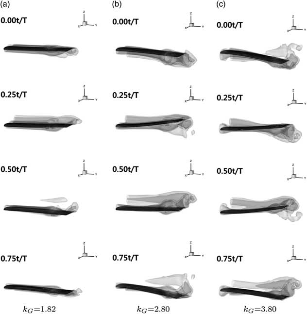
Moreover, the vorticity contours are analysed for the flexible and highly flexible wings in order to comprehend the FSI phenomena more clearly. The relevant results are shown in Figs 14 and 15. Figure 14 shows the vorticity contour around the flexible wing. By increasing k G , a phase shift of the wing tip displacement is clearly shown, and the vorticity is generated around the wing root and tip in upward and downward directions, respectively. Thus, the increasing rate of the averaged thrust is decreased when k G is further increased. Regarding the highly flexible wing, the relevant vorticity contour is shown in Fig. 15. The vorticity is generated around the wing root and tip in upward and downward directions, respectively when k G is 1.82. By increasing k G , the bending behaviour becomes severe, and a strong vorticity is induced. Specifically, the vorticity both near the wing root and tip becomes strong. Moreover, the reverse location changes to the 70% position of the wing span when k G is further increased.

Figure 14 Iso-surfaces of the vorticity magnitude around the flexible wing.

Figure 15 Iso-surfaces of the vorticity magnitude around the highly flexible wing.
As a result, different characteristics are found for the plunging wings when the reduced frequency is further increased. In the flexible wing, a degradation of the averaged thrust is manifested when k G is further increased. A degradation is also found in the highly flexible wing when k G is less than 1.82. Such phenomena are induced by the generation of aerodynamic loads in opposite directions between the wing root and tip. In addition, the reverse location is at the 50% position of the wing span. However, the location changes to the 70% position when k G is further increased, and growth of the aerodynamic loads becomes prominent.
6.0 CONCLUSION
An improved FSI analysis is developed in this study. A CR shell element is developed for a structural analysis, and a relevant non-linear dynamic formulation is developed based on the CR framework. Three-dimensional preconditioned Navier–Stokes equations are employed for a fluid analysis. An implicit coupling scheme is employed to combine the structural and fluid analyses. First, the present FSI analysis is validated by comparing the results with the experimental results. Then, an explicit investigation is conducted for a 3D plunging wing using the present FSI analysis. The novel accomplishments of the present paper can be summarised as follows:
• A non-linear dynamic analysis method based on the CR framework for three-node triangular shell elements is developed.
• The present FSI analysis exploits a wide range of reduced frequencies for a 3D plunging wing to investigate the relevant influence on the interactive phenomena between the fluid and the structure.
• Different characteristics are found for the flexible and highly flexible wings under a high plunging frequency.
Moreover, it is found that a rapid plunging motion induces both a degradation and an increase in the thrust. The degradation is generated by the bending deflection of the highly flexible wing and the following aerodynamic loads in opposite directions between the root and the tip. Moreover, such a degradation is significant when the reversed position of the pressure or vorticity is located at the 50% position of the wing span. However, the characteristics change when the plunging frequency is further increased because of the relocation of the reversed position, which may increase the thrust of the plunging wing. Such a mechanism may be required when the flapping wing is mainly fabricated and operated using an actuator based on polymer and smart materials. However, the high-frequency response in the thrust history of the highly flexible wing must still be investigated. In the future, the present FSI analysis will be further improved by employing a 3D non-linear solid element.
ACKNOWLEDGEMENTS
This work was supported by the Advanced Research Center Program (NRF-2013R1A5A1073861) through a National Research Foundation of Korea (NRF) grant funded by the Korean government (MSIP), contracted through the Advanced Space Propulsion Research Center at Seoul National University and also by the EDISON Program through the National Research Foundation of Korea (NRF) funded by the Ministry of Science, ICT & Future Planning (No. 2014M3C1A6038344).