NOMENCLATURE
- c
-
aerofoil mean aerodynamic chord, m
- CL
-
lift coefficient
- C L0
-
CL value at the mean angle-of-attack
-
 ${C_{L\dot{\alpha }}}$
-
time-delay-of-wash derivative relative to CL
- CLq
-
damping derivative relative to CL
-
${C_{L\dot{\alpha }}} + {C_{Lq}}$
-
combined derivative relative to CL
- Cm
-
moment coefficient
- C m0
-
Cm value at the mean angle-of-attack
-
${C_{m\dot{\alpha }}}$
-
time-delay-of-wash derivative relative to Cm
- Cmq
-
damping derivative relative to Cm
-
${C_{m\dot{\alpha }}} + {C_{mq}}$
-
combined derivative relative to Cm
- CN
-
normal force coefficient
- Dp
-
raindrop diameter, m
- E impact
-
raindrop impact energy,
- FD
-
droplet drag force parameter
- f
-
oscillating frequency, Hz
- gx
-
gravitational acceleration in the x direction, m/s2
- h 0
-
initial film thickness, m
- LWC
-
liquid water content, g/m3
- L
-
lift, N
- M
-
moment, Nm
- q
-
pitching rate, rad/s
-
$\bar{q}$
-
non-dimensional pitching rate
- R
-
rainfall rate, mm/h
- S
-
reference area, m2
- t
-
time, s
- u
-
air velocity in the x direction, m/s
- up
-
raindrop velocity in the x direction, m/s
- ur
-
relative velocity between air and raindrop, m/s
- VT
-
raindrop terminal velocity, m/s
- V ∞
-
freestream air velocity, m/s
- α
-
oscillating angle-of-attack, °
- α0
-
mean oscillating angle-of-attack, °
- Δα
-
amplitude of oscillating angle-of-attack, °
-
$\dot{\alpha }$
-
time rate change of angle-of-attack, rad/s
- σ
-
water surface tension, N/m
- ρ
-
air density, kg/m3
- ρ p
-
raindrop density, kg/m3
- δbl
-
wall boundary-layer thickness, m
- ω
-
oscillating angular velocity, rad/s


1.0 INTRODUCTION
Aerodynamic penalty due to aircraft flying through heavy rain has been deemed to be a critical cause for many severe aviation accidents(Reference Luers and Haines1-Reference Cao, Wu and Xu3). A heavy rain rate of 1,800mm/h can cause a 30% decrease in lift and a 20% increase in drag and can also affect stall angle, boundary-layer separation, flight safety and manoeuvrability(Reference Haines and Luers4). Meteorologists and aeronautical researchers have been interested in rain associated with thunderstorms for decades.
Investigation of rain effect on aircraft flight was begun with the wind-tunnel test, and perhaps the earliest was conducted by Rhode in 1941(Reference Rhode5). His analysis showed that a DC-3 aircraft encountering a rain cloud with Liquid Water Content (LWC) of 50g/m3 would suffer an 18% reduction in the airspeed due to the drag increase associated with the momentum imparted to the aircraft. Haines and Luers studied the frequency and intensity of very heavy rains and their effects on a landing aircraft(Reference Haines and Luers4). Their work showed that heavy rain can not only cause a decrease in maximum lift by 30% but also increase the wing roughness. Hansman and Craig(Reference Hansman and Craig6) compared the aerodynamic performance degradations of the NACA 64–210, NACA 0012 and Wortman FX 67-K170 aerofoils under low Reynolds numbers in a heavy rain condition and explored the underlying mechanisms. As the computer technology is being developed these years, a new way (i.e., numerical simulation) emerges. In 1995, Valentine and Decker(Reference Valentine and Decker7,Reference Valentine and Decker8) numerically studied the NACA 64–210 aerofoil aerodynamic performance and the trajectory of raindrop in rain. Wan's research group(Reference Wan and Wu9-Reference Wan and Pan10) and Margaris's group(Reference Douvi, Margaris, Lazaropoulos and Svanas11,Reference Douvi, Margaris and Lazaropoulos12) conducted a series of work on the prediction of aerofoil aerodynamic performance in rain conditions. Recently, Wu and Cao's research group conducted a series of studies on the aerodynamic performance of various aerofoils and wings and the stability and control characteristics of a DHC-6 Twin Otter aircraft in heavy rain conditions(Reference Ismail, Cao, Bakar and Wu13-Reference Wu, Cao and Ismail16). Their results showed the existence of great degradations of aerodynamic efficiency and flight performance in heavy rain conditions.
As can be seen from above, nearly all the available literatures focus on the effects of rain on aircraft static aerodynamic performance. The only available literature on aircraft dynamic performance comes from our recent work(Reference Wu, Cao and Ismail16) where the longitudinal stability and control characteristics is evaluated for the DHC-6 Twin Otter aircraft. However, the method used in that work is an indirect way where the static aerodynamic performance of the components of the wing and tail plane is simulated and is then substituted into the engineering evaluation formulas to obtain the stability and control derivatives for the complete aircraft. In this article, we present a novel approach to directly calculate the dynamic stability derivatives for a complete transport aircraft in heavy rain conditions. As the workload is quite heavy, we only focus on the longitudinal dynamic characteristics of a complete aircraft model, an approximated DLR-F12 model in the current study. The reason for choosing this plane is that the DLR-F12 model used is a typical geometry of a generic transport aircraft and was constructed specifically for dynamic tests by many research institutions(Reference Mialon, Khelil and Huebner17) and there are a plenty of available static and dynamic aerodynamic data in the available open literatures. Generally, the commercial fluid solver FLUENT(18) is adopted for the whole flowfield calculation, where the heavy rain condition is simulated by using the Discrete Phase Model (DPM) and the unsteady forced oscillation motion is implemented for the aircraft by using the dynamic mesh technique. First of all, the simulated dynamic results in the dry condition are compared with the wind-tunnel experimental data. Afterwards, the DPM model is activated and the dynamic aerodynamic derivatives in the heavy rain condition are calculated.
2.0 METHODOLOGY DESCRIPTION
In the current numerical study, the two-way coupled Eulerian-Lagrangian scheme is used to study the heavy rain effects on both the static and dynamic aerodynamic performances of the DLR-F12 model. The air is treated as the continuous phase and the raindrop as the discrete phase. The air flowfield is derived by solving the incompressible Reynolds Averaged Navier-Stokes (RANS) equations while the raindrop is tracked through air flowfield by solving the Langrangian equations of motion. The rain particles moving in the flow field impinge on the aircraft surface, some of these impinging particles form a thin water layer on the surface and some of these particles are splashed back. We make an assumption in our study that the rain particles striking the aerofoil are non-interacting. It has been shown by Bilanin(Reference Bilanin19) that for a 4mm average diameter raindrop, the mean distance between consecutive raindrops corresponding to a liquid water content of 80g/m3 and a rainfall rate of 1,872mm/h is usually not less than 70mm or 17.5 times the drop diameter, which is thought to be quite a safety distance for the drops to move independently in the falling process. Therefore, it has been assumed for simplicity that the collision of the raindrops are neglected in our simulation. Although there are few specific studies on the uncertainties with this assumption from Bilanin nor from the present authors, this assumption has widely been accepted in this field and the simulation results seem to be good compared with experimental results. In terms of choice of the turbulence model, our previous work(Reference Ismail, Cao, Bakar and Wu13) has shown that for relatively low-Reynolds-number flows, the Spalrat-Allmaras (S-A) turbulence model provides much closer results to the experimental than other more complex turbulence models (e.g., the k-ε turbulence model). Comparisons of the predicted lift and pitching moment using the S-A, k-ε and k-ω turbulence models also proved this conclusion, as can be found in the fourth section. Another advantage of the S-A turbulence model lies in its intrinsic one-equation property, making it require much fewer resources than other turbulence models. Therefore, considering the highly computational resource for the present simulation, the S-A turbulence model is used for our study, with enhanced wall functions incorporated as the near-wall treatment to turbulence.
In most researches of rain, lift coefficient CL and moment coefficient Cm are usually adopted to measure the aerodynamic performance, which are respectively defined as follows:
 $$\begin{equation}
{C_L} = \frac{L}{{\frac{1}{2}\rho {V_\infty }^2S}},\\
\end{equation}$$
$$\begin{equation}
{C_L} = \frac{L}{{\frac{1}{2}\rho {V_\infty }^2S}},\\
\end{equation}$$
 $$\begin{equation}
{C_m} = \frac{M}{{\frac{1}{2}\rho {V_\infty }^2Sc}},
\end{equation}$$
$$\begin{equation}
{C_m} = \frac{M}{{\frac{1}{2}\rho {V_\infty }^2Sc}},
\end{equation}$$
2.1 Modelling of rain conditions
In experimental and numerical simulations, the rainfall rate (R) in millimetre per hour or the liquid water content (LWC) in gram per cubic meter has been chosen to categorise different intensities of rainfall. A rainfall of rate of 100mm/h or greater is often considered heavy rain(Reference Haines and Luers4). The relationship between LWC (g/m3) and R (mm/h) for thunderstorm type rain is given by Ref. (Reference Bezos, Dunham, Gentry and Melson20).
 $$\begin{equation}
{\rm LWC} = 0.054R^{0.84}
\end{equation}$$
$$\begin{equation}
{\rm LWC} = 0.054R^{0.84}
\end{equation}$$
It is assumed that raindrops have been with uniform velocity (i.e., without acceleration) before hitting the aircraft surface. This velocity is called terminal velocity (VT ) of raindrop. It has been developed by Markowitz(Reference Markowitz21) as a function of the raindrop size and altitude. At low altitudes, the terminal velocity of raindrop, which are of interest here, can be written as follows:
 $$\begin{equation}
{V_T}\left( {m/s} \right) = 9.58\left\{ {1 - \exp \left[ { - {{\left( {\frac{{{D_p}}}{{1.77}}} \right)}^{1.147}}} \right]} \right\},
\end{equation}$$
$$\begin{equation}
{V_T}\left( {m/s} \right) = 9.58\left\{ {1 - \exp \left[ { - {{\left( {\frac{{{D_p}}}{{1.77}}} \right)}^{1.147}}} \right]} \right\},
\end{equation}$$
where Dp is the diameter of raindrop.
The trajectory of the discrete raindrop particle is predicted by integrating the force balance on the particle, which is written in a Lagrangian reference frame (for the x direction in Cartesian coordinate) as(18):
 $$\begin{equation}
\frac{{d{u_p}}}{{dt}} = {F_D}(u - {u_p}) + \frac{{{g_x}({\rho _p} - \rho )}}{{{\rho _p}}}
\end{equation}$$
$$\begin{equation}
\frac{{d{u_p}}}{{dt}} = {F_D}(u - {u_p}) + \frac{{{g_x}({\rho _p} - \rho )}}{{{\rho _p}}}
\end{equation}$$
where FD (u − up ) is the drag force per unit particle mass with u and up denoting the x-directional velocities of the air and raindrop, respectively. gx is the x-directional component of the gravitational acceleration. ρ and ρ p stand for the densities of the air and raindrop, respectively.
The mechanism of raindrops impacting onto an aerofoil has been shown in Fig. 1. It is shown in Fig. 1 that some of high-energy rain particles striking on the aerofoil are splashed back into the air while the rest make thin layers of water on the aerofoil surfaces. The back-splashed raindrops at the leading edge form an ejecta fog nearby. These all contribute to the degradation of aerodynamic performance of the aerofoil in heavy rain conditions.

Figure 1. Mechanism of raindrops impacting onto an aerofoil.
In the DPM, the wall film is modelled by injecting the water particles in the air flowfield. The raindrop particles impinge and interact with the wall of the aircraft. In the wall film model, four major interaction regimes are categorised, namely, spread, stick, rebound, and splash. The four wall interaction regimes depend on the impact energy of the impinging raindrops, E impact expressed by:
 $$\begin{equation}
E_{{\rm{impact}}}^2 = \frac{{{\rho _p}{u_r}^{\rm{2}}{D_p}}}{\sigma }\left\{ {\frac{{\rm{1}}}{{{\rm{min(}}{h_0}{\rm{/}}{D_p}{\rm{,1) + }}{\delta _{{\rm{bl}}}}/{D_p}}}} \right\}{\rm{ }}
\end{equation}$$
$$\begin{equation}
E_{{\rm{impact}}}^2 = \frac{{{\rho _p}{u_r}^{\rm{2}}{D_p}}}{\sigma }\left\{ {\frac{{\rm{1}}}{{{\rm{min(}}{h_0}{\rm{/}}{D_p}{\rm{,1) + }}{\delta _{{\rm{bl}}}}/{D_p}}}} \right\}{\rm{ }}
\end{equation}$$
where ur is the relative velocity between the raindrop and the air, h 0 is the initial film thickness, δbl is the wall boundary-layer thickness and σ is the water surface tension.
2.2 Calculation of stability derivatives
Generally, there are a variety of approaches to calculate the parts of the dynamic derivatives. Figure 2 describes an example of the pitching moment due to the pitching motion and the resulting derivatives(Reference Hübner, Bergmann and Loeser22). The pitching motion about the mean value α0 with amplitude Δα generates a hysteresis loop in the aerodynamic response. The bulging out of this hysteresis loop represents the dynamic derivative. In this case, the pitching moment is negative (damping) and the direction of the signal is anti-clockwise. The derivative is the sum of two terms:
 $$\begin{equation}
{C_{m\dot{\alpha }}} = \frac{{\partial {C_m}}}{{\partial (\partial \alpha /\partial t)}}
\end{equation}$$
$$\begin{equation}
{C_{m\dot{\alpha }}} = \frac{{\partial {C_m}}}{{\partial (\partial \alpha /\partial t)}}
\end{equation}$$
 $$\begin{equation}
{C_{mq}} = \frac{{\partial {C_m}}}{{\partial \bar{q}}},
\end{equation}$$
$$\begin{equation}
{C_{mq}} = \frac{{\partial {C_m}}}{{\partial \bar{q}}},
\end{equation}$$
where
 ${C_{m\dot{\alpha }}}$
is an unsteady term describing the influence of wing wash on the horizontal tailplane after a time delay and can be derived by simulating a pure heave oscillation motion shown in the rightmost subgraph of Fig. 2. Cmq
is the quasi-steady damping term representing the pitching moment due to the constant pitching rate q (here, the normalised pitching rate
${C_{m\dot{\alpha }}}$
is an unsteady term describing the influence of wing wash on the horizontal tailplane after a time delay and can be derived by simulating a pure heave oscillation motion shown in the rightmost subgraph of Fig. 2. Cmq
is the quasi-steady damping term representing the pitching moment due to the constant pitching rate q (here, the normalised pitching rate
 $\bar{q} = qc/(2{V_\infty })$
) and can be obtained by simulating a quasi-steady pulling-out motion shown in the middle subgraph of Fig. 2. Thus, the combined derivative
$\bar{q} = qc/(2{V_\infty })$
) and can be obtained by simulating a quasi-steady pulling-out motion shown in the middle subgraph of Fig. 2. Thus, the combined derivative
 ${C_{mq}} + {C_{m\dot{\alpha }}}$
is obtained by summing the results of Cmq
and
${C_{mq}} + {C_{m\dot{\alpha }}}$
is obtained by summing the results of Cmq
and
 ${C_{m\dot{\alpha }}}$
or simply by simulating a pitching oscillation motion as shown in the leftmost subgraph of Fig. 2.
${C_{m\dot{\alpha }}}$
or simply by simulating a pitching oscillation motion as shown in the leftmost subgraph of Fig. 2.

Figure 2. Illustration of dynamic derivatives of the unsteady pitching motion(Reference Hübner, Bergmann and Loeser22).
2.2.1 The combined derivative
${C_{mq}} + {C_{m\dot{\alpha }}}$

In this work, we first obtain the combined derivative
 ${C_{mq}} + {C_{m\dot{\alpha }}}$
by imposing a forced sinusoidal motion around the aircraft's centre of gravity. The forced sinusoidal pitching motion imposed on the aircraft is defined as:
${C_{mq}} + {C_{m\dot{\alpha }}}$
by imposing a forced sinusoidal motion around the aircraft's centre of gravity. The forced sinusoidal pitching motion imposed on the aircraft is defined as:
 $$\begin{equation}
\alpha = {\alpha _0} + \Delta \alpha \sin (\omega t),
\end{equation}$$
$$\begin{equation}
\alpha = {\alpha _0} + \Delta \alpha \sin (\omega t),
\end{equation}$$
where α0 and Δα are the mean angle-of-attack (AOA) and amplitude of oscillating angle-of-attack in the unit of rad/s, respectively. ω = 2πf is the angular velocity where f is the oscillating frequency.
The time rate change of angle-of-attack
 $\dot{\alpha }$
is equal to the non-dimensional pitching rate
$\dot{\alpha }$
is equal to the non-dimensional pitching rate
 $\bar{q}$
written as:
$\bar{q}$
written as:
 $$\begin{equation}
\dot{\alpha } = \omega \Delta \alpha \cos (\omega t) = \bar{q} = qc/(2{V_\infty })
\end{equation}$$
$$\begin{equation}
\dot{\alpha } = \omega \Delta \alpha \cos (\omega t) = \bar{q} = qc/(2{V_\infty })
\end{equation}$$
It is assumed herein that the aerodynamic coefficients are linear functions of the inputs. For the forced oscillation pitch motion, the lift and pitch moment can be written as:
 $$\begin{equation}
{C_L} = {C_{L0}} + {C_{L\alpha }}(\alpha - {\alpha _0}) + ({C_{L\dot{\alpha }}} + {C_{Lq}})\bar{q},\\
\end{equation}$$
$$\begin{equation}
{C_L} = {C_{L0}} + {C_{L\alpha }}(\alpha - {\alpha _0}) + ({C_{L\dot{\alpha }}} + {C_{Lq}})\bar{q},\\
\end{equation}$$
 $$\begin{equation}
{C_m} = {C_{m0}} + {C_{m\alpha }}(\alpha - {\alpha _0}) + ({C_{m\dot{\alpha }}} + {C_{mq}})\bar{q},
\end{equation}$$
$$\begin{equation}
{C_m} = {C_{m0}} + {C_{m\alpha }}(\alpha - {\alpha _0}) + ({C_{m\dot{\alpha }}} + {C_{mq}})\bar{q},
\end{equation}$$
In this study, we present a very simple method for direct calculation of the combined dynamic derivative
 ${C_{m\dot{\alpha }}} + {C_{mq}}$
from the simulated forced oscillation motion(Reference Ghoreyshi, Bergeron, Lofthouse and Cummings23). Taking the pitching moment as an example, the pitching moment changes during a complete sinusoidal pitching motion make a quasi-steady elliptical hysteresis as illustrated in the leftmost subgraph of Fig. 2. There exists two points where the angular velocity reaches the minimum and maximum at α = α0. The maximum and minimum angular velocities equal to + ωΔα and − ωΔα, respectively. Marking the pitching moment values at the two specific points as C
m+ and C
m−, respectively. Substituting C
m+ and C
m− in Equation (12) obtains:
${C_{m\dot{\alpha }}} + {C_{mq}}$
from the simulated forced oscillation motion(Reference Ghoreyshi, Bergeron, Lofthouse and Cummings23). Taking the pitching moment as an example, the pitching moment changes during a complete sinusoidal pitching motion make a quasi-steady elliptical hysteresis as illustrated in the leftmost subgraph of Fig. 2. There exists two points where the angular velocity reaches the minimum and maximum at α = α0. The maximum and minimum angular velocities equal to + ωΔα and − ωΔα, respectively. Marking the pitching moment values at the two specific points as C
m+ and C
m−, respectively. Substituting C
m+ and C
m− in Equation (12) obtains:
 $$\begin{equation}
{C_{m + }} = {C_{m0}} + ({C_{m\dot{\alpha }}} + {C_{mq}})\frac{{\omega c\Delta \alpha }}{{2{V_\infty }}}\\
\end{equation}$$
$$\begin{equation}
{C_{m + }} = {C_{m0}} + ({C_{m\dot{\alpha }}} + {C_{mq}})\frac{{\omega c\Delta \alpha }}{{2{V_\infty }}}\\
\end{equation}$$
 $$\begin{equation}
{C_{m - }} = {C_{m0}} - ({C_{m\dot{\alpha }}} + {C_{mq}})\frac{{\omega c\Delta \alpha }}{{2{V_\infty }}}
\end{equation}$$
$$\begin{equation}
{C_{m - }} = {C_{m0}} - ({C_{m\dot{\alpha }}} + {C_{mq}})\frac{{\omega c\Delta \alpha }}{{2{V_\infty }}}
\end{equation}$$
Subtract Equation (14) from Equation (13) and we can obtain the combined derivative:
 $$\begin{equation}
{C_{m\dot{\alpha }}} + {C_{mq}} = \frac{{{C_{m + }} - {C_{m - }}}}{{2k\Delta \alpha }},
\end{equation}$$
$$\begin{equation}
{C_{m\dot{\alpha }}} + {C_{mq}} = \frac{{{C_{m + }} - {C_{m - }}}}{{2k\Delta \alpha }},
\end{equation}$$
where
 $k = \frac{{wc}}{{2{V_\infty }}}$
is the reduced frequency.
$k = \frac{{wc}}{{2{V_\infty }}}$
is the reduced frequency.
In this study, the above pitching oscillation motion of the DLR-F12 is implemented by adopting the dynamic mesh technique associated with the User-Defined Function (UDF). More details about the application of the dynamic mesh technique as well as the UDF can be found in Ref. 18 and for brevity it is omitted here.
2.2.2 The damping derivative Cmq
Second, we calculate the damping derivative Cmq by solving a quasi-steady pulling-out motion as shown in the middle subgraph of Fig. 2. It defines a circular motion for the aircraft flying with unvaried velocity, angle-of-attack and pitching rate. Although this motion does not objectively exist, the aircraft angle-of-attack keeps constant under this motion, thus can be used to identify the damping derivative Cmq . To realise this motion, from the relative movement point of view, we can add a rotating reference frame where the rotating rate equals the pitching rate. The distance between the aircraft centre of gravity and the origin of the coordinate is
 $$\begin{equation}
R = \frac{{{V_\infty }}}{q}
\end{equation}$$
$$\begin{equation}
R = \frac{{{V_\infty }}}{q}
\end{equation}$$
This quasi-steady pulling-out motion is simulated by using the rotating reference frame technique. Calculate the corresponding pitching moment coefficients C m1 and C m2 with two different values of pitching rate q 1 and q 2, and then we can obtain the damping derivative by
 $$\begin{equation}
{C_{mq}} = \frac{{{C_{m1}} - {C_{m2}}}}{{{{\bar{q}}_1} - {{\bar{q}}_2}}}
\end{equation}$$
$$\begin{equation}
{C_{mq}} = \frac{{{C_{m1}} - {C_{m2}}}}{{{{\bar{q}}_1} - {{\bar{q}}_2}}}
\end{equation}$$
2.2.3 The time-delay-of-wash derivative
${C_{m\dot{\alpha }}}$

Finally, we obtain the unsteady derivative
 ${C_{m\dot{\alpha }}}$
via a simple mathematical subtraction operation, i.e.,
${C_{m\dot{\alpha }}}$
via a simple mathematical subtraction operation, i.e.,
 $$\begin{equation}
{C_{m\dot{\alpha }}} = ({C_{m\dot{\alpha }}} + {C_{mq}}) - {C_{mq}}
\end{equation}$$
$$\begin{equation}
{C_{m\dot{\alpha }}} = ({C_{m\dot{\alpha }}} + {C_{mq}}) - {C_{mq}}
\end{equation}$$
The other dynamic derivatives about the lift can be calculated in a similar fashion as shown above.
3.0 VALIDATION OF THE NUMERICAL ALGORITHM
3.1 Dynamic performance prediction
To validate the capability of the flow solver and the dynamic mesh technique approach described above, the standard AGARD test case(Reference Landon24) of the NACA 0012 aerofoil is taken as the test case. Here we present the calculated results for the unsteady flow past the NACA 0012 aerofoil undergoing pitching oscillation motions about the quarter chord under the conditions of AGARD CT1 and AGARD CT5(Reference Landon24), whose test conditions are shown as follows, AGARD CT1:
 $$\begin{equation*}
{{\rm M}_\infty } = 0.6,\;{\rm Re} = 4.8 \times {10^6},\;{\alpha _0} = 2.89^\circ ,\;\Delta \alpha \ = 2.41^\circ ,\;k = 0.0808
\end{equation*}$$
$$\begin{equation*}
{{\rm M}_\infty } = 0.6,\;{\rm Re} = 4.8 \times {10^6},\;{\alpha _0} = 2.89^\circ ,\;\Delta \alpha \ = 2.41^\circ ,\;k = 0.0808
\end{equation*}$$
AGARD CT5:
 $$\begin{equation*}
{{\rm M}_\infty } = 0.755,\;{\rm Re} = 5.5 \times {10^6},\;{\alpha _0} = 0.016^\circ ,\;\Delta \alpha = 2.51^\circ ,\;k = 0.0814,
\end{equation*}$$
$$\begin{equation*}
{{\rm M}_\infty } = 0.755,\;{\rm Re} = 5.5 \times {10^6},\;{\alpha _0} = 0.016^\circ ,\;\Delta \alpha = 2.51^\circ ,\;k = 0.0814,
\end{equation*}$$
where M∞ is Mach number and Re is Reynolds number.
Figures 3 and 4, respectively, show the comparison of the computed results for the normal force coefficient CN and pitching moment coefficient Cm with the density and momentum terms separately discretised by the first-order upwind scheme and the second-order upwind scheme and the wind-tunnel experimental values for the NACA 0012 aerofoil under the AGARD CT1 condition. We can see that the dynamic mesh technique approach proposed in this article is valid to simulate unsteady circular pitching oscillation motions. Besides, it is clear that the numerical results with the second-order discretisation scheme show a better agreement with the experimental results. The maximum uncertainties of CN associated with the first-order and the second-order upwind schemes are approximately 12% and 5% at typical angles of attack. Thus, the second-order discretisation scheme is adopted for all the following calculations. Furthermore, Figs 5 and 6 present the comparison for the NACA 0012 aerofoil under the AGARD CT5 test condition, which also shows a relatively good capability of the current approach for dynamic aerodynamic performance prediction.
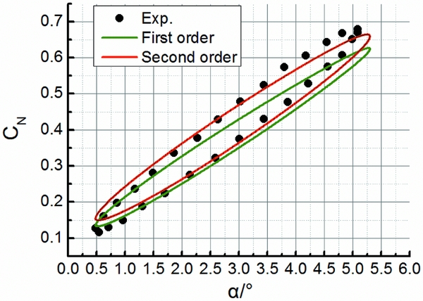
Figure 3. Comparison of normal force coefficient CN for AGARD CT1.

Figure 4. Comparison of pitching moment coefficient Cm for AGARD CT1.

Figure 5. Comparison of normal force coefficient CN for AGARD CT5.
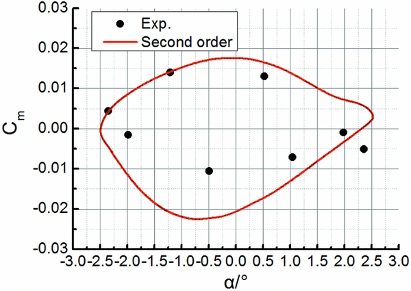
Figure 6. Comparison of pitching moment coefficient Cm for AGARD CT5.
3.2 Rain environment simulation
To verify the capability of the DPM to predict aircraft aerodynamic performance in rain environment, we present the simulation results of lift coefficient for a rectangular wing with aspect ratio of 2 in the heavy rain condition in Fig. 7. The experimental data is acquired from Hansman and Craig's wind-tunnel test(Reference Hansman and Craig6) and the numerical results are extracted from our group's previous work(Reference Ismail, Cao, Wu and Sohail14). The rain condition is associated with LWC of 30g/m3. The turbulence model corresponds to the S-A model. As can be seen from Fig. 7, the lift coefficient of the wing decreases in rain at most of the low to middle angles of attack of interest. As for the experimental results, the maximum percentage decrease in lift coefficient reaches 17% in the rain condition, while for our simulation results, the corresponding value reaches up to 18%. This decrease in lift is caused by the thin layer of water formed on the upper and lower surfaces of the wing and the splashed-back particles produced due to high-energy impact of water particles with the wall of the wing. The film layer on the wing, cratering by droplet impact, instability, and breakup into rivulets, they all interact with the turbulent boundary-layer dynamics.

Figure 7. Comparison of lift coefficient CL for the rain simulation model.
4.0 RESULTS AND DISCUSSIONS
In this section, we are studying the static and dynamic aerodynamics for the DLR-F12 model aircraft in the dry and rain conditions, respectively. Due to the unavailability of the DLR-F12 model, this article uses a similar open DLR-F6 model downloaded from the NASA website(Reference Vassberg, DeHaan, Rivers and Wahls25), which belongs to the family of DLR F-series standard models and might be regarded as an acceptable approximation of the accurate DLR-F12 model. We generate the DLR-F12 model by adding a vertical tail with an arbitrary symmetrical profile (NACA 0012 in this study), since the vertical tail does not affect the longitudinal derivatives much. Here, a half-scale model is used for study of the longitudinal aerodynamic performance due to the symmetry of the model in the longitudinal direction. The geometric parameters for the half-scale model is listed in Table 1. The reference frame is illustrated in Fig. 8.
Table 1 Geometric parameters of the DLR-F12 model

Figure 8. Global view of the computational domain for the DLR-F12 model (top) and amplified view of mesh refinement near the lifting surfaces (bottom).
In terms of the mesh strategy, an unstructured grid is adopted around the half DLR-F12 model in the present study, as shown in Fig. 8. The mesh is generated in ANSYS ICEM, which is a professional mesh generator for both structured and unstructured meshes. Grid density technique is adopted around the lifting surface, e.g., the wing, the horizontal and the vertical tailplanes, which can produce a much finer mesh in a specific local region. The standard mesh for the overall subsequent study has totally about 3.24 million elements and 0.56 million nodes. In terms of the boundary condition, the blue plane, which is located in the symmetric plane of the aircraft, is set as symmetry, as well as the other outermost domain in red set as velocity inlet. The overall aircraft wall surface is set as no-slip wall.
4.1 Aerodynamic coefficients/derivatives in the dry condition
Numerical simulations are first conducted on static test conditions in order to check the ability of the tools to match static aerodynamic forces. Angles of attack from –5° to 5.2° for longitudinal flows are considered. For all the following static and dynamic computations, the freestream velocity of air is set to be 70m/s. To ensure the numerical result is independent of the mesh, a much finer mesh with totally about 5.47 million and 0.98 million nodes is also adopted for calculation.
The numerical results for the two meshes as well as the experimental results from Ref. (Reference Mialon, Khelil and Huebner17) are plotted in Figs 9 and 10. First of all, it can be seen from the two figures that the difference between the lift and moment results calculated with the standard and the refined meshes has reached a negligible level. Second, the slope of lift coefficient is well predicted by the current simulation. A shift of around 1° of angle-of-attack exists between the numerical and experimental lift curves, which in the authors’ opinion is a normal reflection of the difference between wind-tunnel experiments and numerical simulations. Thus, this angle-of-attack difference usually considered and calibrated before simulations is not necessarily calibrated in the current study since the current study focuses on the effect of rainfall on the dynamic performance. The above difference of lift coefficient consequently causes the difference in the moment coefficient between the experiment and the current simulation shown in Fig. 10. In addition, there is also some difference between the numerical and experimental slopes of moment curve.

Figure 9. Comparison of lift coefficient CL in the dry condition.

Figure 10. Comparison of moment coefficient Cm in the dry condition.
To reveal the effect of alternative turbulence models on the prediction, comparisons of the predicted lift and pitching moment using the S-A, k-ε, and k-ω turbulence models are made and shown in Tables 2 and 3. Generally, the S-A turbulence model provides a better prediction accuracy than the other two turbulence models, proving that the S-A turbulence model is better suited for the present low-speed flow simulations.
Table 2 Comparison of CL between the experimental results and the numerical results using various turbulence models

Table 3 Comparison of Cm between the experimental results and the numerical results using various turbulence models
Figure 11 shows the values of y + at three different spanwise stations of the wing (as also illustrated) for the two meshes. Associating with the aerodynamic performance shown in Figs 9 and 10, it is found that though the finer mesh generally obtains nearly half of the y + values of the standard mesh, it does not bring a conspicuous improvement on the predicted aerodynamic forces and moments needed. This implies that, with the enhanced wall functions employed in the turbulence model, the near-wall mesh resolution can be somewhat compromised whereas the aerodynamic coefficients are not much affected.

Figure 11. y +values at different wing wall positions (distinguished by the colours) obtained by the standard mesh (solid) and the finer mesh (hollow).
We then first calculate the quasi-steady dynamic derivatives by using the aforementioned method with two values of 23 and 15rad/s selected for the pitching rate q and present the corresponding results for the lift coefficient CL
and moment coefficient Cm
in Table 4. Using the data in Table 4 and the form of Equation (17), we obtain the numerical steady dynamic derivatives CLq
and Cmq
and compare with the results from the wind-tunnel experiment and other Navier-Stokes (NS) numerical tools(Reference Mialon, Khelil and Huebner17), as plotted in Fig. 12. Note that the experimental data include the contribution for
 $\dot{\alpha }$
derivatives. Although our predicted CLq
is larger while all the others are less than the experimental result, it is clear that our result has the least error with respect to the experimental result. In general, our simulation results achieve equally good agreement with the experimental results as other numerical studies.
$\dot{\alpha }$
derivatives. Although our predicted CLq
is larger while all the others are less than the experimental result, it is clear that our result has the least error with respect to the experimental result. In general, our simulation results achieve equally good agreement with the experimental results as other numerical studies.
Table 4 Calculation results for the two pitching rates selected
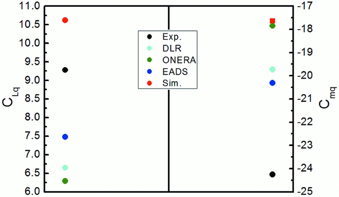
Figure 12. Steady dynamic derivatives obtained with various tools in the dry condition.
For the combined dynamic derivatives
 ${C_{Lq}} + {C_{L\dot{\alpha }}}$
, a forced pitching oscillation motion is imposed on the DLR-F12 model. The testing condition is as follows:
${C_{Lq}} + {C_{L\dot{\alpha }}}$
, a forced pitching oscillation motion is imposed on the DLR-F12 model. The testing condition is as follows:
 $$\begin{equation*}
{V_\infty } = 70{\rm{ }}m/s,\;{\alpha _0} = 0^\circ ,\;\Delta \alpha = 4.52^\circ ,\;f = 3{\rm{ }}Hz,\;k = 0.068.
\end{equation*}$$
$$\begin{equation*}
{V_\infty } = 70{\rm{ }}m/s,\;{\alpha _0} = 0^\circ ,\;\Delta \alpha = 4.52^\circ ,\;f = 3{\rm{ }}Hz,\;k = 0.068.
\end{equation*}$$
The time evolutions of the numerical and experimental lift force and pitching moment are plotted in Fig. 13. The plotted signals are obtained by subtracting the mean value of the computed signal in one period and then divided by the experimental amplitude. A shift of about 1/10th of the period between the lift and pitching moment curves is observed for both the simulation and the experiment. The prediction on the lift coefficient is very satisfactory. For the pitching moment, the current simulation results slightly underestimate the maximum values. Despite it, the phase difference between both signals (lift and pitching moment) is perfectly predicted.
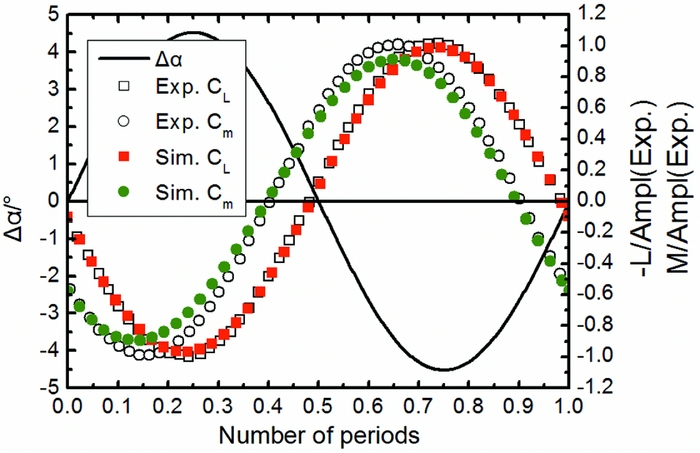
Figure 13. Time History of lift force and pitching moment coefficients in the dry condition.
The unsteady combine dynamic derivatives are then derived and plotted in Fig. 14. These results include the
 $\dot{\alpha }$
contribution and thus are directly comparable to the experimental data. Now compared with the results obtained by the other numerical tools, it is clear that our simulation result reaches the best agreement with the experimental results for the lift derivative. However, the agreement is worse for the pitching moment. The
$\dot{\alpha }$
contribution and thus are directly comparable to the experimental data. Now compared with the results obtained by the other numerical tools, it is clear that our simulation result reaches the best agreement with the experimental results for the lift derivative. However, the agreement is worse for the pitching moment. The
 ${C_{L\dot{\alpha }}}$
(
${C_{L\dot{\alpha }}}$
(
 ${C_{m\dot{\alpha }}}$
, respectively) contribution computed with our CFD approach is negative and in the region of 29.57% (12.98%, respectively) of the CLq
(Cmq
, respectively) value. Therefore, it can be important to take these components into account in the aircraft aerodynamic model because they can lead to significant errors in longitudinal flight dynamics criteria (e.g., short-period incidence oscillation).
${C_{m\dot{\alpha }}}$
, respectively) contribution computed with our CFD approach is negative and in the region of 29.57% (12.98%, respectively) of the CLq
(Cmq
, respectively) value. Therefore, it can be important to take these components into account in the aircraft aerodynamic model because they can lead to significant errors in longitudinal flight dynamics criteria (e.g., short-period incidence oscillation).
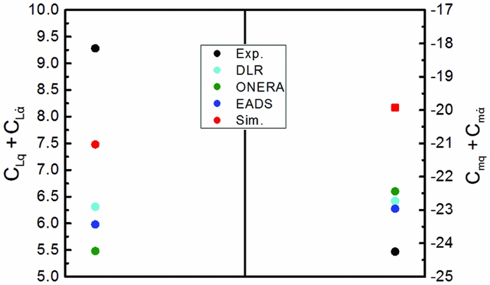
Figure 14. Unsteady combined dynamic derivatives obtained with various tools in the dry condition.
4.2 Aerodynamic coefficients/derivatives in the wet condition
In this section, the DPM is activated to simulate the aerodynamic performance in heavy rain. The rainfall conditions adopted for study are associated with LWC of 30g/m3, raindrop diameter of 1mm, raindrop terminal velocity of 4m/s.
The CFD results of static aerodynamic lift and moment coefficients for the DLR-F12 in the dry and rain conditions are shown in Figs 15 and 16. It can be seen that both CL and Cm show a well linear relationship as a function of α in the range of angle-of-attack of interest. However, both the magnitudes of the slope of CL and Cm (i.e., C Lα and C mα) decrease under the heavy rain condition, which is consistent with our previous study(Reference Ismail, Wu, Bakar and Tariq26). As is shown in Table 5 for the static and dynamic derivatives in the dry and rain conditions, C Lα and C mα experienced a reduction of about 15% and 18% in rain, respectively. In addition, both the lift and moment coefficients also decrease in the heavy rain condition for a specific angle-of-attack. The maximum percentage of lift coefficient decrease arrives at 33% at angle-of-attack of –3° and the maximum percentage of moment coefficient decrease went up to 25% at angle-of-attack of 3°. It can be easily imagined that this rain-induced static aerodynamic performance degradation makes an aircraft require more energy from the engines to accelerate so that the lost lift can be compensated to balance the weight of the aircraft.
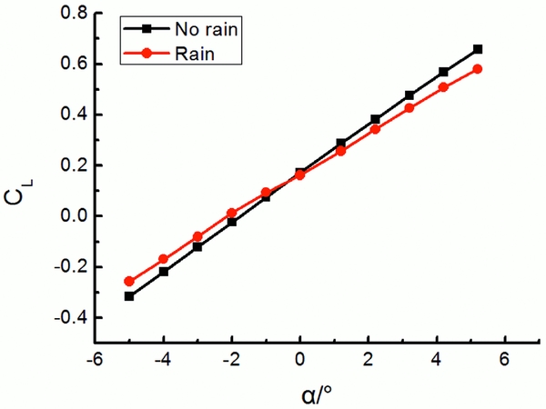
Figure 15. Comparison of the simulated static lift coefficient CL between the dry and wet conditions.

Figure 16. Comparison of the simulated static moment coefficient Cm between the dry and wet conditions.
Table 5 Comparison of the calculated results for the dynamic derivatives between the dry and wet conditions

Figures 17 and 18, respectively, plot the loops of the integrated aerodynamic coefficients against the instantaneous angle-of-attack with the same forced oscillation motion as in the last section imparted to the model under the dry and wet conditions. A difference for both the lift and moment coefficients between the no-rain and rain conditions can be clearly seen. Generally, the magnitude of the lift and moment coefficients as well as their slopes decreases in the wet condition.

Figure 17. Comparison of the simulated dynamic lift coefficient CL between the dry and wet conditions for a full oscillation period.
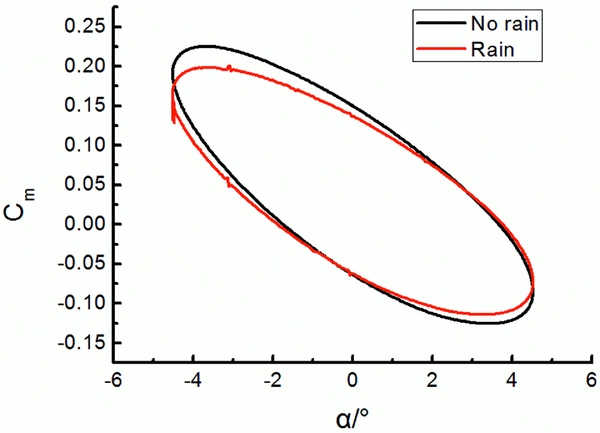
Figure 18. Comparison of the simulated dynamic moment coefficient Cm between the dry and wet conditions for a full oscillation period.
Combining the data in Figs 17 and 18 and the form of Equation (15), we obtain the values of the combined dynamic derivative
 ${C_{Lq}} + {C_{L\dot{\alpha }}}$
and
${C_{Lq}} + {C_{L\dot{\alpha }}}$
and
 ${C_{mq}} + {C_{m\dot{\alpha }}}$
in the no-rain and rain conditions. Table 5 summarises the predicted results of the static and dynamic derivatives for the DLR-F12 aircraft in the dry and wet conditions. In this table, the negative value represents the degradation of the parameter in rain compared with no rain. All the parameters exhibit different-level degradations except the lift-related combined derivative
${C_{mq}} + {C_{m\dot{\alpha }}}$
in the no-rain and rain conditions. Table 5 summarises the predicted results of the static and dynamic derivatives for the DLR-F12 aircraft in the dry and wet conditions. In this table, the negative value represents the degradation of the parameter in rain compared with no rain. All the parameters exhibit different-level degradations except the lift-related combined derivative
 ${C_{Lq}} + {C_{L\dot{\alpha }}}$
. Of all these parameters, the two unsteady
${C_{Lq}} + {C_{L\dot{\alpha }}}$
. Of all these parameters, the two unsteady
 $\dot{\alpha }$
derivatives
$\dot{\alpha }$
derivatives
 ${C_{L\dot{\alpha }}}$
and
${C_{L\dot{\alpha }}}$
and
 ${C_{m\dot{\alpha }}}$
undergo a significant percentage degradation of over 30% in the heavy rain condition compared with the dry case. Considering that the α and q responses, which are representative of the short-period mode, closely depend on
${C_{m\dot{\alpha }}}$
undergo a significant percentage degradation of over 30% in the heavy rain condition compared with the dry case. Considering that the α and q responses, which are representative of the short-period mode, closely depend on
 ${C_{L\dot{\alpha }}}$
and
${C_{L\dot{\alpha }}}$
and
 ${C_{m\dot{\alpha }}}$
, it can be concluded that the short-period mode flight performance of the aircraft will be significantly affected, which is consistent with the conclusion obtained by our previous work(Reference Wu, Cao and Ismail16).
${C_{m\dot{\alpha }}}$
, it can be concluded that the short-period mode flight performance of the aircraft will be significantly affected, which is consistent with the conclusion obtained by our previous work(Reference Wu, Cao and Ismail16).
5.0 CONCLUSIONS
Heavy rain has many adverse effects on aircraft flight performance and can cause more engine energy consumption. In this article, we initially study the dynamic aerodynamic performance of a transport aircraft in heavy rain environment. A novel approach is introduced to directly calculate the longitudinal stability derivatives for the DLR-F12 model in heavy rain conditions. A discrete phase model is adopted to simulate the heavy rain condition and the unsteady forced oscillation motion is implemented by using the dynamic mesh technique to calculate the dynamic derivatives for the DLR-F12 model.
As for the approach proposed in this article, our simulation results show a good agreement with corresponding experimental data for both the static and dynamic aerodynamic performances. As for the heavy rain effect, the results indicate that both the static and dynamic aerodynamic performances suffer significant degradations in the heavy rain condition. On the one hand, in terms of the static aerodynamic performance, a maximum percentage of 33% lift coefficient decrease and a maximum percentage of 25% moment coefficient decrease are predicted in heavy rain. Besides, the slopes of both the lift and moment curves also decrease by about 15% and 18% in rain, respectively. This rain-induced aerodynamic performance degradation makes an aircraft require more energy from the engines to accelerate so that the lost lift can be compensated to balance the weight of the aircraft. On the other hand, in regard to the dynamic aerodynamic performance, the majority of the derivatives exhibit different-level degradations. The two unsteady time-delay-of-wash derivatives
 ${C_{L\dot{\alpha }}}$
and
${C_{L\dot{\alpha }}}$
and
 ${C_{m\dot{\alpha }}}$
undergo a significant percentage degradation of over 30% in the heavy rain condition compared with the dry case. This new finding suggests that the short-period mode flight performance of an aircraft may greatly suffer in heavy rain environment, since the α and q responses, which are representative of the short-period mode, closely depend on
${C_{m\dot{\alpha }}}$
undergo a significant percentage degradation of over 30% in the heavy rain condition compared with the dry case. This new finding suggests that the short-period mode flight performance of an aircraft may greatly suffer in heavy rain environment, since the α and q responses, which are representative of the short-period mode, closely depend on
 ${C_{L\dot{\alpha }}}$
and
${C_{L\dot{\alpha }}}$
and
 ${C_{m\dot{\alpha }}}$
. These results are new and may be useful for people to recognise and understand heavy rain effects on aircraft flight performance and energy consumption.
${C_{m\dot{\alpha }}}$
. These results are new and may be useful for people to recognise and understand heavy rain effects on aircraft flight performance and energy consumption.
FUNDINGS
Financial support has been provided by the National Natural Science Foundation of China (grant number 11702014).