NOMENCLATURE
Roman symbols
- A
sectional aero
- E
elastic modulus
- f
natural frequency
- G
shear modulus
- H
the thickness of the simplified cylindrical shell
- I
sectional moment of inertia
- k
shear coefficient
- l
axial length of the stiffened cylindrical shell
- N
the quantity of stiffeners
- R
mid-radius of the stiffened cylindrical shell
- R j
the distance between the jth stiffener and the x-axis of the cross section
- x
the direction along the axis of beam
- y
the lateral displacement of beam
Greek symbols
- δ
thickness of the stiffened cylindrical shell
- ε
the error of similarity
- λ
scale factor
- ν
Poisson’s ratio
- ρ
density
Subscripts
- ()0
referring to a single stiffener
- ()1
referring to the shell
- ()2
referring to all stiffeners
- () m
referring to the model
- ()pre
referring to the predicted value of the scaled model for the prototype
- ()pro
referring to the prototype
- ()sim
referring to the simplified cylindrical shell
1.0 INTRODUCTION
Thin-walled cylindrical shell has the advantages of lightweight, small thickness and large bending rigidity. It is widely used in aerospace, shipbuilding, military equipment, oil transportation, civil construction and many other fields. Especially in the launch vehicle, a large number of stiffened (such as milled) cylindrical shells are used as the main load-bearing structures such as propellant tanks. The structural vibrational characteristics of the stiffened cylindrical shells, which account for two-third of the total length of launch vehicle, need to be verified to ensure the accuracy of dynamical model for the whole launcher. On the other hand, considering the large size of the launch vehicle, it is not only expensive to use the full-size model test, but also required high testing equipment and site. In order to reduce the technical risk and cost, shorten the development cycle and be easy to use the existing testing technique, scaling model tests are usually carried out before the project is formally implemented to verify the feasibility of the scheme( Reference Coutinho, Baptista and Dias Rodrigues 1 ).
The theoretical basis of scaling model test is similarity theory, whose core is to deduce scaling laws to guide the design of scaling model. The traditional dimensional analysis and equational analysis are the most commonly used methods for deriving scaling laws. Krayterman and Sabnis( Reference Krayterman and Sabnis 2 ) applied dimensional analysis to deduce scaling laws of plate and cylinder, in which the influence of boundary conditions on the scaling laws is considered and the accuracy of the similarity method is discussed. Morgen( Reference Morgen 3 ) studied the similarity of orthogonal stiffened cylindrical shells under different static loads. It is concluded that equational analysis is more suitable for the similarity study of orthogonal stiffened cylindrical shells than dimensional analysis. Soedel( Reference Soedel 4 ) used equational analysis to derive the exact scaling laws and approximate scaling laws of the vibrating shell. Based on the analysis of the Love equation of shell, the scaling laws of the two dominant cases of the stretching effect and the bending effect are derived, respectively.
The corresponding scaled models above fully satisfy the scaling laws derived from traditional similarity method, so they are called completely similarity models. However, restrained from practical conditions, human factors or other reasons, the scaled model is probably not satisfy one or several conditions in scaling laws. This type of scaled model is called partial similarity model (or incomplete similarity model) and the unsatisfied conditions are known as similarity distortion( Reference Coutinho, Baptista and Dias Rodrigues 1 ). In general, since the response or characteristic of partial similarity model has a large deviation from the prototype in terms of similarity, it is necessary to correct the similarity distortion. In engineering, the application requirements of the partial similarity models or distortion models are more extensive than that of the completely similarity model. But at present, there are few theoretical studies on similarity distortions, and the related research only stays at the level of the analysis of the influence on similarity in some specific object, and there are few systematic and general methods for dealing with similarity distortion. Chouchaoui and Ochoa( Reference Chouchaoui and Ochoa 5 ) applied equational analysis to develop scaling laws for the cases of laminated cylindrical tubes subject to tensile, torsion, bending, internal and external pressure loads. Not content with the restrictions on the design of parameters of completely similarity model, the influence of parameters change on scaling laws is studied. The partial similarity models are designed with different stacking sequences, number of plies and geometric parameters. The influence of these parameters on the similarity of the response parameters is calculated by numerical analysis. Furthermore, it is shown that in the deduced range of values of these parameters, the scaled model keeps accurate prediction of the behaviour of the prototype. Similarly, Torkamani et al.( Reference Torkamani, Navazi and Jafari 6 ) used dimensional analysis to derive the free vibration scaling laws for an orthotropic stiffened cylindrical shell. The change of scaling laws and experimental verification of the partial similarity model, such as replacing material of cylindrical shell, adjusting the sectional size of stiffeners and changing the quantity of stiffeners, are carried out. In the above two references, the research related to the partial similarity model is to analyse the influence of the model parameters on the similarity of the response results. This kind of analysis is applied more in field of composite structures, such as a series of studies on the structural similarity of composites by Yazdi and Rezaeepazhand( Reference Yazdi and Rezaeepazhand 7 – Reference Rezaeepazhand and Wisnom 11 ). Especially in some references( Reference Ferro 12 – 16 ), this process of analysis is called analysis of self-similar. However, this analysis only determines the range of model parameters when the similarity distortion has little effect in partial similarity model by parametric sensitivity analysis and does not really correct the similarity distortion.
Based on the above researches, Luo et al( Reference Luo, Zhu and Zhao 17 – Reference Zhu, Luo and Zhao 19 ) used equational analysis to derive the complete scaling laws and the incomplete scaling laws of the natural frequency and the vibration response for the thin-walled cylindrical shell. In the study of the partial similarity models for the change of geometric parameters such as radius, wall thickness and length of cylindrical shells, the function of scale factor of frequency on the scale factor of three geometric parameters is set in a form of power. This function is regarded as incomplete scaling laws, whose exponents are the undetermined parameters and finally determined by parametric sensitivity analysis and fitting calculation. Compared to the study( Reference Chouchaoui and Ochoa 5 , Reference Torkamani, Navazi and Jafari 6 ), this paper further used the results of parameter sensitivity analysis to establish more accurate incomplete scaling laws. However, one of the most widely used applications of scaled model test is that experimental studies are needed because the object is difficult to simulate accurately through theoretical or numerical calculations. In this case, the problem that accuracy of the data is uncertain exists in the parametric sensitivity analysis based on numerical calculation in the paper. So this method can be applied to fewer objects of scaled model test.
Rosa and Franco studied analytical similitudes applied to thin cylindrical shells( Reference Rosa and Franco 20 ). The work is focused on the definition and the analysis of both complete and incomplete similitudes for the dynamic responses of thin shells. These similitudes and the associated scaling laws are defined by using the classical modal approach and by invoking also the energy distribution approach in order to take into account both the cinematic and energetic items. However, the derived scaling law of stiffened cylindrical shells is too harsh for the parameter design of scaled model, so it is difficult to meet the requirement of large scale-down model for launch vehicles.
Cho( Reference Cho 21 ) presented and continuously developed a novel empirical similitude method: the empirical similarity method (ESM). By designing product specimen and model specimen as the transitional models, the ESM can deal with some of similarity distortions( Reference Tadepalli and Wood 22 – Reference Tadepalli and Wood 25 ). The ESM is universal and can be applied to the study of similarity of stiffened cylindrical shells. However, because some of the key assumptions in the ESM have no definite basis, and it is impossible to judge the accuracy of these assumptions according to the specific object, the similarity precision of the method cannot be predicted, controlled and improved.
In the above studies related to the similarity of stiffened cylindrical shell (or cylindrical shell), the traditional similarity methods are used to derive scaling laws, as a result, the problem of similarity distortion cannot be solved effectively. In the few studies involving partial similarity models, there has not been a relatively systematic and general method for dealing with similarity distortion. Therefore, this paper takes the stiffened cylindrical shell as the research object. In view of the limitation of the scaling laws derived by traditional dimensional analysis, an equivalent similarity method is proposed to solve the problem of similarity distortion and to make the design of scaled model more freely.
2.0 SIMILARITY DISTORTION AND EQUIVALENT SIMILAR METHOD
As shown in Fig. 1, the stiffened cylindrical shell is taken as a research object, which consists of the shell and a total of N axial stiffeners with arbitrary sectional shape distributed equidistantly in the circumference. The relevant parameters including axial length, mid-radius, thickness, sectional aero, sectional moment of inertia, elastic modulus, shear modulus, density, Poisson’s ratio and natural frequency are represented as l, R, δ, A, I, E, G, ρ, ν and f, respectively. In the following, subscripts ‘0’, ‘1’ and ‘2’ denote a single stiffener, the shell and all stiffeners, respectively.
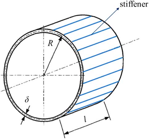
Figure 1 (Colour online) Geometry of the stiffened cylindrical shell.
In addition, the scale factor λ of PARM (parameter) is defined as the ratio of its prototype value to its model value, that is,
 $${\rlambda }{\equals}{{{\rm PARM}_{m} } \over {{\rm PARM}_{{{\rm pro}}} }}$$
where subscripts ‘pro’ and ‘m’ represent the prototype and the model, respectively.
If the scale factor of axial length λ l for stiffened cylindrical shell is 1/20, and with dimensional analysis, then the scale factors of other size parameters must also be equal to 1/20, which derives
 $$ \left\{ \matrix{ {\rm \rlambda }_{R} {\equals}{\rm \rlambda }_{\rdelta } {\equals}{\rm \rlambda }_{l} {\equals}{1 \over {20}} \hfill \cr {\rm \rlambda }_{{A_{0} }} {\equals}{\rm \rlambda }_{l}^{2} {\equals}{1 \over {20^{2} }} \hfill \cr {\rm \rlambda }_{{I_{0} }} {\equals}{\rm \rlambda }_{l}^{4} {\equals}{1 \over {20^{4} }} \hfill \cr} \right.$$
However, considering that thickness of the shell and cross-sectional dimensions of stiffeners in the launch vehicle are usually very small, it is impossible to process such a 1/20 scaled model according to the current manufacturing capacity, that is, there is a problem of similar distortion. This problem arises from the limitations of the dimension analysis. To be precise, dimension analysis requires that the scale factors of the parameters with same dimension must be uniform.
In this paper, an equivalent similar method is proposed to solve the similarity distortion caused by a series of practical limitations, such as the above-mentioned manufacturing capacity, material selection, experimental conditions and so on. The method is as follow: Simplify the governing equation through equivalent process, where some parameters of the object are integrated at first in order to reduce the amount of parameters involved in equational analysis, and thus simplify the scaling laws, eliminate similarity distortion and make the design of scaled model more freely.
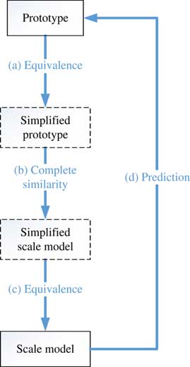
The concrete steps of this method are shown in Fig. 2, that is
a) The prototype is equivalent to a simplified prototype through establishing the equivalent criteria.
b) The scaling laws of the simplified prototype are derived, and a simplified scaled model satisfying the complete similarity is designed.
c) The scaled model is equivalent designed based on the simplified scaled model, where the same equivalent criterion as the (a) process can be used.
d) The behaviour of the prototype can be predicted by use of the test result of the scaled model and the derived scaling laws.
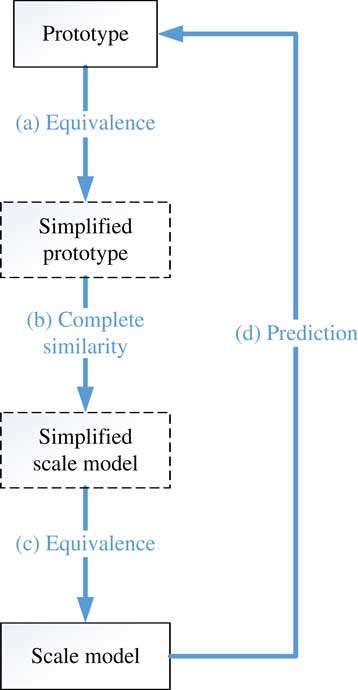
Figure 2 (Colour online) Process of the equivalent method.
Thus, with simplified object as a transition, scaling laws with complex structure can be established indirectly through the above way of ‘equivalent + similar +equivalent’. It should be noted that the simplified prototype and simplified scaled model are virtual transitional models, that is, there is no need for the model to test, which is essentially different from the ESM.
3.0 EQUIVALENT SCALING LAWS OF TRANSVERSE BENDING MODE
In the following part, the scaling laws of global bending mode for stiffened cylindrical shell would be derived through the equivalent similar method proposed in the previous section. First, we establish the equivalent criteria, then deduce the scaling laws and finally analyse the advantages of the equivalent similarity.
3.1 Process of equivalence
To achieve the equivalence of global bending mode, cylindrical shell without stiffeners is chosen as simplified object (simplified prototype and simplified scaled model). Thus, it is necessary to establish the equivalent criteria from the stiffened cylindrical shell to a cylindrical shell without stiffeners. The transversal free vibrational differential equation of cylindrical shell based on the hypothesis of Timoshenko Beam is( 26 )
 $${\rm \rrho }A{{\partial ^{2} y(x,t)} \over {\partial t^{2} }}{\plus}EI{{\partial ^{4} y(x,t)} \over {\partial x^{4} }}{\minus}{\rm \rrho }I\left[ {1{\plus}{{(EI)({\rm \rrho }A)} \over {k(GA)({\rm \rrho }I)}}} \right]{{\partial ^{4} y(x,t)} \over {\partial x^{2} \partial t^{2} }}{\plus}{{({\rm \rrho }A)({\rm \rrho }I)} \over {k(GA)}}{{\partial ^{2} y(x,t)} \over {\partial t^{4} }}{\equals}0$$
where x donates the direction along the axis of beam, y is the lateral displacement of beam and k is the shear coefficient.
From Equation (3), we know that ρA, EI, ρI and GA are the ‘equivalent parameters’. Then, the four equivalent parameters are analysed as follows.
In terms of the equivalent parameter EI, the relationship between the stiffened cylindrical shell and the simplified cylindrical shell can be represented as
 $$E_{{{\rm sim}}} I_{{{\rm sim}}} {\equals}E_{1} I_{1} {\plus}E_{2} I_{2}$$
or
 $$E_{{{\rm sim}}} {\rm \rpi }HR_{{{\rm sim}}}^{3} {\equals}E_{1} {\rm \rpi \rdelta }R^{3} {\plus}E_{2} I_{2}$$
where the subscript ‘sim’ refers to the simplified cylindrical shell and H represents the thickness of the simplified cylindrical shell. It is assumed that the simplified cylindrical shell has the same elastic modulus and midface radius as the shell of the stiffened cylindrical shell, that is
 $$\left\{ \matrix{ E_{{{\rm sim}}} {\rm {\equals}}E_{1} \hfill \cr R_{{{\rm sim}}} {\rm {\equals}}R \hfill \cr} \right.$$
By substituting Equation (6) into Equation (5), the expression of H is obtained
 $$H{\equals}{\rm \rdelta }{\plus}{{E_{2} I_{2} } \over {E_{1} I_{1} }}{\rm \rdelta }$$
In terms of the equivalent parameter ρA, the relationship between the stiffened cylindrical shell and the simplified cylindrical shell can be represented as
 $${\rm \rrho }_{{{\rm sim}}} A_{{{\rm sim}}} {\equals}{\rm \rrho }_{1} A_{1} {\plus}{\rm \rrho }_{2} A_{2}$$
where the cross-sectional areas can be further expressed as
 $$\left\{ \matrix{ A_{{{\rm sim}}} {\rm {\equals}}2{\rm \rpi }HR \hfill \cr A_{1} {\equals}2{\rm \rpi \rdelta }R \hfill \cr A_{2} {\equals}NA_{0} \hfill \cr} \right.$$
Then by simplifying Equation (8) with Equation (9), the density of the simplified cylindrical shell ρsim can be expressed as
 $${\rm \rrho }_{{{\rm sim}}} {\equals}{{2{\rm \rpi \rdelta }R{\rm \rrho }_{1} {\plus}NA_{0} {\rm \rrho }_{2} } \over {2{\rm \rpi }HR}}$$
In terms of the equivalent parameter ρI, the relationship between the stiffened cylindrical shell and the simplified cylindrical shell can be represented as
 $${\rm \rrho '}_{{{\rm sim}}} I_{{{\rm sim}}} {\equals}{\rm \rrho }_{1} I_{1} {\plus}{\rm \rrho }_{2} I_{2}$$
where ρ′sim represents the equivalent density of the simplified cylindrical shell through the equivalent parameter ρI. Meanwhile, ρI of the shell and the stiffeners can be expressed, respectively, as( Reference Xing, Pan and Yang 27 )
 $${\rm \rrho }_{1} I_{1} {\rm {\equals}\rrho }_{1} A_{1} R^{2} \,/\,2$$
 $${\rm \rrho }_{2} I_{2} {\rm {\equals}\rrho }_{2} \left( {NI_{0} {\plus}A_{0} \mathop{\sum}\limits_{j{\equals}1}^N {R_{j}^{2} } } \right)\,\approx\,{\rm \rrho }_{2} A_{0} \mathop{\sum}\limits_{j{\equals}1}^N {R_{j}^{2} } $$
where R
j
represents the distance between the j
th stiffener and the x-axis of the cross section, NI
0 is smaller than
 $$A_{0} \mathop{\sum}\nolimits_{j{\equals}1}^N {R_{j}^{2} } $$
and can be ignored. When enough stiffeners are arranged equidistantly along the circumference, Equation (13) can be simplified as
$$A_{0} \mathop{\sum}\nolimits_{j{\equals}1}^N {R_{j}^{2} } $$
and can be ignored. When enough stiffeners are arranged equidistantly along the circumference, Equation (13) can be simplified as
 $${\rm \rrho }_{2} I_{2} \,\approx\,{\rm \rrho }_{2} A_{0} \mathop{\sum}\limits_{j{\equals}1}^N {R_{j}^{2} } {\rm {\equals}\rrho }_{2} A_{0} NR^{2} \,/\,2$$
By substituting Equations (12) and (14) into Equation (11), the expression of ρ′sim is obtained
 $${\rm \rrho '}_{{{\rm sim}}} {\rm {\equals}}\;{\rm \rrho }_{{{\rm sim}}} $$
Equation (15) shows that the equivalent density derived from the equivalent parameters ρA and ρI is the same, that is, the two equivalent parameters are equivalent.
In terms of the equivalent parameter GA, the relationship between the stiffened cylindrical shell and the simplified cylindrical shell can be represented as
 $$G_{{{\rm sim}}} A_{{{\rm sim}}} {\equals}G_{1} A_{1} {\plus}G_{2} A_{2} $$
By substituting Equation (8) into Equation (16), next Equation (17) is obtained
 $$G_{{{\rm sim}}} {\equals}G_{1} {{{\rm \rdelta }{\plus}{{G_{2} } \over {G_{1} }}{{NA_{0} } \over {A_{1} }}{\rm \rdelta }} \over H}$$
Meanwhile, according to Equations (12) and (14),
 $${{I_{1} } \over {I_{2} }}$$
is represented as
$${{I_{1} } \over {I_{2} }}$$
is represented as
 $${{I_{1} } \over {I_{2} }}{\equals}{{A_{1} R^{2} \,/\,2} \over {NA_{0} R^{2} \,/\,2}}$$
that is,
 $${{I_{1} } \over {I_{2} }}{\equals}{{A_{1} } \over {NA_{0} }}$$
By substituting Equation (19) into Equation (17), the shear modulus of the simplified cylindrical shell G sim can be expressed as
 $$G_{{{\rm sim}}} {\equals}G_{1} {{{\rm \rdelta }{\plus}{{G_{2} E_{1} } \over {G_{1} E_{2} }}{{E_{2} I_{2} } \over {E_{1} I_{1} }}{\rm \rdelta }} \over H}$$
Then, by substituting Equation (7) into Equation (20), G sim is simplified as
 $$G_{{{\rm sim}}} {\equals}G_{1} {{{\rm \rdelta }{\plus}{{G_{2} E_{1} } \over {G_{1} E_{2} }}\left( {H{\minus}{\rm \rdelta }} \right)} \over H}$$
At last, synthesising the above derivation obtains the simplified cylindrical shell with axial length l, mid-radius R, thickness H, Young’s modulus of elasticity E 1, shear modulus G sim and density ρsim. Equations (7), (10) and (21) are the expression of H, ρsim and G sim, respectively.
3.2 Calculation of scaling laws
The next step is to derive the scaling laws of complete similarity. By applying the equational analysis to Equation (3), the sub-items, including
 $${\rm \rrho }A{{\partial ^{2} y(x,t)} \over {\partial t^{2} }}$$
,
$${\rm \rrho }A{{\partial ^{2} y(x,t)} \over {\partial t^{2} }}$$
,
 $$EI{{\partial ^{4} y(x,t)} \over {\partial x^{4} }}$$
,
$$EI{{\partial ^{4} y(x,t)} \over {\partial x^{4} }}$$
,
 $${\rm \rrho }I{{\partial ^{4} y(x,t)} \over {\partial x^{2} \partial t^{2} }}$$
,
$${\rm \rrho }I{{\partial ^{4} y(x,t)} \over {\partial x^{2} \partial t^{2} }}$$
,
 $${{{\rm \rrho }I(EI)({\rm \rrho }A)\partial ^{4} y(x,t)} \over {k(GA)({\rm \rrho }I)\partial x^{2} \partial t^{2} }}$$
and
$${{{\rm \rrho }I(EI)({\rm \rrho }A)\partial ^{4} y(x,t)} \over {k(GA)({\rm \rrho }I)\partial x^{2} \partial t^{2} }}$$
and
 $${{({\rm \rrho }A)({\rm \rrho }I)\partial ^{2} y(x,t)} \over {k(GA)\partial t^{4} }}$$
, should have the same value of scale factor, that is,
$${{({\rm \rrho }A)({\rm \rrho }I)\partial ^{2} y(x,t)} \over {k(GA)\partial t^{4} }}$$
, should have the same value of scale factor, that is,
 $${{{\rm \rlambda }_{{\rm \rrho }} {\rm \rlambda }_{A} {\rm \rlambda }_{y} } \over {{\rm \rlambda }_{t}^{2} }}{\equals}{{{\rm \rlambda }_{E} {\rm \rlambda }_{I} {\rm \rlambda }_{y} } \over {{\rm \rlambda }_{l}^{4} }}{\equals}{{{\rm \rlambda }_{{\rm \rrho }} {\rm \rlambda }_{I} {\rm \rlambda }_{y} } \over {{\rm \rlambda }_{l}^{2} {\rm \rlambda }_{t}^{2} }}{\equals}{{{\rm \rlambda }_{{\rm \rrho }} {\rm \rlambda }_{I} ({\rm \rlambda }_{E} {\rm \rlambda }_{I} )({\rm \rlambda }_{{\rm \rrho }} {\rm \rlambda }_{A} ){\rm \rlambda }_{y} } \over {{\rm \rlambda }_{k} ({\rm \rlambda }_{G} {\rm \rlambda }_{A} )({\rm \rlambda }_{{\rm \rrho }} {\rm \rlambda }_{I} ){\rm \rlambda }_{l}^{2} {\rm \rlambda }_{t}^{2} }}{\equals}{{({\rm \rlambda }_{{\rm \rrho }} {\rm \rlambda }_{A} )({\rm \rlambda }_{{\rm \rrho }} {\rm \rlambda }_{I} ){\rm \rlambda }_{y} } \over {{\rm \rlambda }_{k} ({\rm \rlambda }_{G} {\rm \rlambda }_{A} ){\rm \rlambda }_{t}^{4} }}$$
By substituting the relevant parameters of the simplified cylindrical shell into Equation (22), the following equations are obtained:
 $${{{\rm \rlambda }_{{{\rm \rrho }_{{{\rm sim}}} }} {\rm \rlambda }_{R} {\rm \rlambda }_{H} {\rm \rlambda }_{y} } \over {{\rm \rlambda }_{t}^{2} }}{\equals}{{{\rm \rlambda }_{{E_{1} }} {\rm \rlambda }_{R}^{3} {\rm \rlambda }_{H} {\rm \rlambda }_{y} } \over {{\rm \rlambda }_{l}^{4} }}$$
 $${{{\rm \rlambda }_{{{\rm \rrho }_{{{\rm sim}}} }} {\rm \rlambda }_{R} {\rm \rlambda }_{H} {\rm \rlambda }_{y} } \over {{\rm \rlambda }_{t}^{2} }}{\equals}{{{\rm \rlambda }_{{{\rm \rrho }_{{{\rm sim}}} }} {\rm \rlambda }_{R}^{3} {\rm \rlambda }_{H} {\rm \rlambda }_{y} } \over {{\rm \rlambda }_{l}^{2} {\rm \rlambda }_{t}^{2} }}$$
 $${{{\rm \rlambda }_{{{\rm \rrho }_{{{\rm sim}}} }} {\rm \rlambda }_{R}^{3} {\rm \rlambda }_{H} {\rm \rlambda }_{y} } \over {{\rm \rlambda }_{l}^{2} {\rm \rlambda }_{t}^{2} }}{\rm {\equals}}{{{\rm \rlambda }_{{{\rm \rrho }_{{{\rm sim}}} }} {\rm \rlambda }_{{E_{1} }} {\rm \rlambda }_{R}^{3} {\rm \rlambda }_{H} {\rm \rlambda }_{y} } \over {{\rm \rlambda }_{k} {\rm \rlambda }_{{G_{{{\rm sim}}} }} {\rm \rlambda }_{l}^{2} {\rm \rlambda }_{t}^{2} }}$$
 $${{{\rm \rlambda }_{{{\rm \rrho }_{{{\rm sim}}} }} {\rm \rlambda }_{R} {\rm \rlambda }_{H} {\rm \rlambda }_{y} } \over {{\rm \rlambda }_{t}^{2} }}{\rm {\equals}}{{{\rm \rlambda }_{{{\rm \rrho }_{{{\rm sim}}} }}^{2} {\rm \rlambda }_{R}^{3} {\rm \rlambda }_{H} {\rm \rlambda }_{y} } \over {{\rm \rlambda }_{k} {\rm \rlambda }_{{G_{{{\rm sim}}} }} {\rm \rlambda }_{t}^{4} }}$$
By simplifying Equation (24), next Equation (22) is obtained
 $${\rm \rlambda }_{R} {\rm {\equals}}\;{\rm \rlambda }_{l} $$
Further, substituting Equation (27) into Equation (23) obtains
 $${\rm \rlambda }_{f} {\equals}{\rm \rlambda }_{t}^{{{\minus}1}} {\equals}{1 \over {{\rm \rlambda }_{l} }}\sqrt {{{{\rm \rlambda }_{{E_{1} }} } \over {{\rm \rlambda }_{{{\rm \rrho }_{{{\rm sim}}} }} }}} $$
After simplifying Equation (25), next Equation (29) is obtained
 $${{{\rm \rlambda }_{{E_{1} }} } \over {{\rm \rlambda }_{k} {\rm \rlambda }_{{G_{{{\rm sim}}} }} }}{\equals}1$$
As the cross section of the simplified prototype and that of the simplified scaled model are both circular rings, therefore, λ k = 1, Equation (29) can be simplified to obtain
 $${\rm \rlambda }_{{E_{1} }} {\rm {\equals}}\;{\rm \rlambda }_{{G_{{{\rm sim}}} }} $$
Meanwhile, Poisson’s ratio of the simplified cylindrical shell is represented as
 $${\rm \nu }_{{{\rm sim}}} {\equals}{{E_{1} {\rm {\minus}}2G_{{{\rm sim}}} } \over {2G_{{{\rm sim}}} }}$$
The scale factor of νsim is expressed as
 $${\rm \rlambda }_{{{\rm \nu }_{{{\rm sim}}} }} {\equals}{\rm \rlambda }_{{{{E_{1} {\rm {\minus}}2G_{{{\rm sim}}} } \over {2G_{{{\rm sim}}} }}}} {\rm {\equals}}{{{\rm \rlambda }_{{E_{1} {\rm {\minus}}2G_{{{\rm sim}}} }} } \over {{\rm \rlambda }_{{2G_{{{\rm sim}}} }} }}$$
Then, according to similitude theory( 28 ), when Equation (30) is satisfied, next Equation (33) is obtained
 $${\rm \rlambda }_{{E_{1} {\rm {\minus}}2G_{{{\rm sim}}} }} {\rm {\equals}\rlambda }_{{E_{1} }} {\rm {\equals}\rlambda }_{{2G_{{{\rm sim}}} }} $$
By substituting Equation (33) into Equation (32),
 $${\rm \rlambda }_{{{\rm \nu }_{{{\rm sim}}} }} $$
can be simplified as
$${\rm \rlambda }_{{{\rm \nu }_{{{\rm sim}}} }} $$
can be simplified as
 $${\rm \rlambda }_{{{\rm \nu }_{{{\rm sim}}} }} {\equals}1$$
In addition, since Equation (26) can be obtained by substituting Equations (27) and (29) into Equation (23), there are no independent scaling laws derived from Equation (26).
Finally, by integrating Equations (27), (28) and (34), the scaling laws of the bending mode for the simplified cylindrical shell which satisfies the hypothesis of Timoshenko Beam are as follows:
 $$\left\{ \matrix{ {\rm \rlambda }_{f} {\equals}{1 \over {{\rm \rlambda }_{l} }}\sqrt {{{{\rm \rlambda }_{{E_{1} }} } \over {{\rm \rlambda }_{{{\rm \rrho }_{{{\rm sim}}} }} }}} \hfill \cr {\rm \rlambda }_{R} {\rm {\equals}\rlambda }_{l} \hfill \cr {\rm \rlambda }_{k} {\equals}1 \hfill \cr {\rm \rlambda }_{{{\rm \nu }_{{{\rm sim}}} }} {\equals}1 \hfill \cr} \right.$$
3.3 Analysis of the equivalent similarity
To sum up, the process of equivalence is established in Fig. 2 and the equivalent criteria given by Equations (7), (10) and (21) are obtained. Through the deduce of scaling laws, we have completed the process of complete similarity in Fig. 2, and we derived the scaling laws given by Equation (35). Thus, the equivalent similarity, that is established by combining these equivalent criteria and scaling laws, is used to design scaled model for global bending mode of the stiffened cylindrical shells, and on the other hand, to predict the global bending mode of the prototype according to that of the scaled model.
Furthermore, this equivalent similarity is thoroughly analysed. Substituting Equations (4) and (16) into the expression of νsim given by Equation (31) yields
 $${\rm \nu }_{{{\rm sim}}} {\equals}{1 \over 2}{{{{E_{1} I_{1} {\plus}E_{2} I_{2} } \over {2{\rm \rpi }R^{3} H}}} \mathord{\left/ {\vphantom {{{{E_{1} I_{1} {\plus}E_{2} I_{2} } \over {2{\rm \rpi }R^{3} H}}} {{{G_{1} A_{1} {\plus}G_{2} A_{2} } \over {2{\rm \rpi }RH}}}}} \right. \kern-\nulldelimiterspace} {{{G_{1} A_{1} {\plus}G_{2} A_{2} } \over {2{\rm \rpi }RH}}}}{\minus}1$$
Equation (36) can be written also using Equation (13) as
 $${\rm \nu }_{{{\rm sim}}} {\equals}{1 \over 2}{{E_{1} } \over {G_{1} }}{{1{\plus}{{E_{2} A_{0} } \over {E_{1} A_{1} }}{{\mathop{\sum}\limits_{j{\equals}1}^N {R_{j}^{2} } } \over {R^{2} }}} \over {1{\plus}{{G_{2} A_{0} } \over {G_{1} A_{1} }}N}}{\minus}1$$
Then, according to similitude theory( 28 ), by substituting Equation (37) into Equation (34), now Equation (38) is obtained
 $$\left\{ \matrix{ {{{\rm \rlambda }_{{E_{1} }} } \over {{\rm \rlambda }_{{G_{1} }} }}{\equals}1 \hfill \cr {{{\rm \rlambda }_{{E_{2} }} {\rm \rlambda }_{{A_{0} }} } \over {{\rm \rlambda }_{{E_{1} }} {\rm \rlambda }_{{A_{1} }} }}{{\vskip--5pt \left. {{\rm \rlambda }_{x} } \right} {\vskip--3pt \big|}{{}_{{x{\equals}\mathop{\scale65%\sum}\limits_{j{\equals}1}^N {R_{j}^{2} }}}} \over {{\rm \rlambda }_{R}^{2} }}{\equals}1 \hfill \cr {{{\rm \rlambda }_{{G_{2} }} {\rm \rlambda }_{{A_{0} }} {\rm \rlambda }_{N} } \over {{\rm \rlambda }_{{G_{1} }} {\rm \rlambda }_{{A_{1} }} }}{\equals}1 \hfill \cr} \right.$$
or
 $$\left\{ \matrix{ {\rm \rlambda }_{{{\rm \nu }_{{\rm 1}} }} {\equals}1 \hfill \cr {\rm \rlambda }_{{{\rm \nu }_{{\rm 2}} }} {\equals}{{{\rm \rlambda }_{N} {\rm \rlambda }_{R}^{2} } \over {\vskip--5pt \left. {{\rm \rlambda }_{x} } \right} {\vskip--3pt \scale 90%\big|}{{}_{{x{\equals}\mathop{\scale65%\sum}\limits_{j{\equals}1}^N {R_{j}^{2} }}}}}{\rm } \hfill \cr {\rm \rlambda }_{{G_{1} }} {\rm \rlambda }_{{A_{1} }} {\rm {\equals}\rlambda }_{{G_{2} }} {\rm \rlambda }_{{A_{0} }} {\rm \rlambda }_{N} \hfill \cr} \right.$$
For the commonly used metal materials in vehicle launchers, the difference between their Poisson’s ratios is very small, that is,
 $${\rm \rlambda }_{{{\rm \nu }_{{\rm 2}} }} {\rm {\equals}}{{{\rm \rlambda }_{{E_{2} }} } \over {{\rm \rlambda }_{{G_{2} }} }}{\rm {\equals}}1$$
Then Equation (39) can be written also by using Equation (40) as
 $$\left\{ \matrix{ {\rm \rlambda }_{{{\rm \nu }_{1} }} {\equals}{\rm \rlambda }_{{{\rm \nu }_{2} }} {\equals}1 \hfill \cr {\rm \rlambda }_{N} {\rm \rlambda }_{R}^{2} \vskip-0pt {\equals} {\vskip--0pt {{\rm \rlambda }_{x} } } {\vskip-2pt \scale 90%\big|}{\vskip---5pt {}_{{x{\equals}\mathop{\scale65%\sum}\limits_{j{\equals}1}^N {R_{j}^{2} }}}} \hfill \cr {\rm \rlambda }_{{E_{1} }} {\rm \rlambda }_{{A_{1} }} {\equals}{\rm \rlambda }_{{E_{2} }} {\rm \rlambda }_{{A_{0} }} {\rm \rlambda }_{N} \hfill \cr} \right.$$
where
 $${\rm \rlambda }_{N} {\rm \rlambda }_{R}^{2} {\equals}\left. {{\rm \rlambda }_{x} } \right \vskip-2pt\big|_{\vskip-10pt {{x{\equals}\mathop{\sum}\nolimits_{j{\equals}1}^N {R_{j}^{2} } }} $$
represents the scaling law relevant to the distribution of the stiffeners.
$${\rm \rlambda }_{N} {\rm \rlambda }_{R}^{2} {\equals}\left. {{\rm \rlambda }_{x} } \right \vskip-2pt\big|_{\vskip-10pt {{x{\equals}\mathop{\sum}\nolimits_{j{\equals}1}^N {R_{j}^{2} } }} $$
represents the scaling law relevant to the distribution of the stiffeners.
The following is a division of Equation (41) in two specific equations used to solve different examples.
(1) If the number and distribution of stiffeners in the scaled model are exactly the same as those of the prototype, it means
 $$\left. {{\rm \rlambda }_{x} } \right|_{{x{\equals}\mathop{\sum}\nolimits_{j{\equals}1}^N {R_{j}^{2} } }} {\equals}\mathop{\sum}\nolimits_{j{\equals}1}^N {{\rm \rlambda }_{{R_{j} }}^{2} } ,\;{\rm \rlambda }_{N} {\equals}1$$
. Therefore, Equation (41) is simplified as
$$\left. {{\rm \rlambda }_{x} } \right|_{{x{\equals}\mathop{\sum}\nolimits_{j{\equals}1}^N {R_{j}^{2} } }} {\equals}\mathop{\sum}\nolimits_{j{\equals}1}^N {{\rm \rlambda }_{{R_{j} }}^{2} } ,\;{\rm \rlambda }_{N} {\equals}1$$
. Therefore, Equation (41) is simplified as
 $$\left\{ \matrix{ {\rm \rlambda }_{{{\rm \nu }_{1} }} {\equals}{\rm \rlambda }_{{{\rm \nu }_{2} }} {\equals}1 \hfill \cr {\rm \rlambda }_{R}^{2} {\equals}\mathop{\sum}\limits_{j{\equals}1}^N {\rlambda _{{R_{j} }}^{2} } \hfill \cr {\rm \rlambda }_{{E_{1} }} {\rm \rlambda }_{{A_{1} }} {\equals}{\rm \rlambda }_{{E_{2} }} {\rm \rlambda }_{{A_{0} }} \hfill \cr} \right.$$
Since
 $${\rm \rlambda }_{R}^{2} {\equals}\mathop{\sum}\nolimits_{j{\equals}1}^N {{\rm \rlambda }_{{R_{j} }}^{2} } $$
in Equation (42) is always satisfied in this case, it no longer needs to be listed. Accordingly, the scaling laws are obtained by using Equations (35) and (42) as
$${\rm \rlambda }_{R}^{2} {\equals}\mathop{\sum}\nolimits_{j{\equals}1}^N {{\rm \rlambda }_{{R_{j} }}^{2} } $$
in Equation (42) is always satisfied in this case, it no longer needs to be listed. Accordingly, the scaling laws are obtained by using Equations (35) and (42) as
 $$\left\{ \matrix{ {\rm \rlambda }_{f} {\equals}{1 \over {{\rm \rlambda }_{l} }}\sqrt {{{{\rm \rlambda }_{{E_{1} }} } \over {{\rm \rlambda }_{{{\rm \rrho }_{{{\rm sim}}} }} }}} \; \hfill \cr {\rm \rlambda }_{R} {\equals}{\rm \rlambda }_{l} \hfill \cr {\rm \rlambda }_{{{\rm \nu }_{{\rm 1}} }} {\equals}{\rm \rlambda }_{{{\rm \nu }_{{\rm 2}} }} {\equals}1 \hfill \cr {\rm \rlambda }_{{E_{1} }} {\rm \rlambda }_{{A_{1} }} {\equals}{\rm \rlambda }_{{E_{2} }} {\rm \rlambda }_{{A_{0} }} \hfill \cr} \right.$$
(2) It is assumed that the prototype has 50 stiffeners and that only 20 stiffeners are designed in the scaled model, it means N pro=50, N m =20. Therefore, Equation (41) is simplified as
 $$\left\{ \matrix{ {\rm \rlambda }_{{{\rm \nu }_{{\rm 1}} }} {\rm {\equals}\rlambda }_{{{\rm \nu }_{{\rm 2}} }} {\rm {\equals}1} \hfill \cr {\vskip4pt{{20} \over {50}}{\rm \rlambda }_{R}^{2} {\equals}\left. {{\rm \rlambda }_{x} } \right\Big|}_{{x{\equals}\mathop{\sum}\limits_{j{\equals}1}^N {R_{j}^{2} } }} \hfill \cr {\rm \rlambda }_{{E_{1} }} {\rm \rlambda }_{{A_{1} }} {\equals}{{20} \over {50}}{\rm \rlambda }_{{E_{2} }} {\rm \rlambda }_{{A_{0} }} \hfill \cr} \right.$$
where
 $${{20} \over {50}}{\rm \rlambda }_{R}^{2} {\equals}\left. {{\rm \rlambda }_{x} } \right\Big|_{{x{\equals}\mathop{\sum}\limits_{j{\equals}1}^N {R_{j}^{2} } }} $$
can be rewritten as
$${{20} \over {50}}{\rm \rlambda }_{R}^{2} {\equals}\left. {{\rm \rlambda }_{x} } \right\Big|_{{x{\equals}\mathop{\sum}\limits_{j{\equals}1}^N {R_{j}^{2} } }} $$
can be rewritten as
 $${{20} \over {50}}{{R_{m}^{2} } \over {R_{{{\rm pro}}}^{2} }}{\equals}{{\left. {\mathop{\sum}\limits_{j{\equals}1}^N {R_{j}^{2} } } \right|_{m} } \over {\left. {\mathop{\sum}\limits_{j{\equals}1}^N {R_{j}^{2} } } \right|_{{{\rm pro}}} }}$$
Similar to the simplification of Equation (14), now Equation (46) is obtained
 $$\left. {\mathop{\sum}\limits_{j{\equals}1}^N {R_{j}^{2} } } \right|_{{{\rm pro}}} {\equals}25R_{{{\rm pro}}}^{2} $$
By substituting Equation (46) into Equation (45), next Equation (47) is obtained
 $$\left. {\mathop{\sum}\limits_{j{\equals}1}^N {R_{j}^{2} } } \right|_{{m}} {\equals}10R_{{m}}^{2} $$
Finally, by integrating Equations (35), (44) and (47), the scaling laws in this special case are obtained as
 $$\left\{ \matrix{ {\rm \rlambda }_{f} {\equals}{1 \over {{\rm \rlambda }_{l} }}\sqrt {{{{\rm \rlambda }_{{E_{1} }} } \over {{\rm \rlambda }_{{{\rm \rrho }_{{{\rm sim}}} }} }}} \hfill \cr {\rm \rlambda }_{R} {\equals}{\rm \rlambda }_{l} \hfill \cr {\rm \rlambda }_{{{\rm \nu }_{{\rm 1}} }} {\rm {\equals}\rlambda }_{{{\rm \nu }_{{\rm 2}} }} {\equals}1 \hfill \cr \left. {\mathop{\sum}\limits_{j{\equals}1}^N {R_{j}^{2} } } \right|_{m} {\equals}10R_{m}^{2} \hfill \cr {\rm 2}{\rm .5\rlambda }_{{E_{1} }} {\rm \rlambda }_{{A_{1} }} {\equals}{\rm \rlambda }_{{E_{2} }} {\rm \rlambda }_{{A_{0} }} \hfill \cr} \right.$$
In summary, the above analysis shows that the scaling laws relevant to the thickness of the cylindrical shell and the section size of the stiffener are reduced in Equation (35). Only the scaling laws between the cross-sectional area, the amount and the distribution of the stiffener are retained. Compared to traditional similarity method, the stiffeners in scaled model are no longer required to maintain the same amount and distribution as the prototype. Moreover, since Equation (35) does not limit the sectional shape of the stiffeners, then the stiffeners of scaled model can be designed with different cross-sectional shapes with that of the prototype. As a consequence, Equation (35) can make the design of scaled model more freely.
4.0 DESIGN OF SCALED MODELS AND VALIDATION OF THE SCALING LAWS
4.1 Design of scaled models
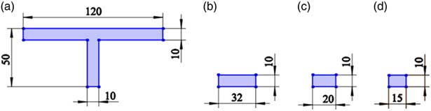
As the finite element model shown in Fig. 3, a stiffened cylindrical shell is set as the prototype with mid-radius of the shell R=2 m, axial length l=40 m and thickness δ=80 mm. Fifty axial stiffeners are distributed equidistantly in the circumference. The geometrical parameters of T-shaped cross section of stiffeners are shown in Fig. 4(a). The shell and the stiffeners are both made of aluminium alloy with elastic modulus 70 GPa, density 2700 kg/m3 and Poisson’s ratio 0.3.
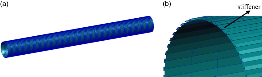
Figure 3 (Colour online) Finite element model of the prototype. (a) Overall view; (b) Partial view.

Figure 4 (Colour online) Cross sections of the stiffeners in the prototype and the scaled models. (a) Prototype; (b) Model-1; (c) Model-2; (d) Model-3.
According to the scaling laws (Equation (35)), three models with different scales are established, which are Models 1, 2 and 3, respectively. In order to verify the analysis of equivalent similarity in Section 3.3, the Model 1 is designed with the same thickness as the prototype, the quantity of stiffeners of the Model 2 is different from that of prototypes and the cylindrical shell and the stiffener in the Model 3 are composed of different materials. Moreover, the cross-sectional shape of the stiffeners of the three models is different from that of the prototype, and the simpler rectangle shape is adopted (as shown in Fig. 4). The related parameters and scaling factors of each model are shown in Tables 1 and 2, respectively. The relevant design is presented in the next paragraph.
(i) According to Equation (43), a 1/5 scaled model named Model 1 is designed. Its mid-radius is 0.4 m, the axial length is 8 m and the thickness is 80 mm the same as the prototype. Fifty axial stiffeners are distributed equidistantly in the circumference. Their cross sections are rectangular with a width of 32 mm and a height of 10 mm (as shown in Fig. 4(b)). The shell and the stiffeners are both made of aluminium alloy. Accordingly, the scaling factors of Model 1 are obtained and shown in Table 2. By substituting the relevant scaling factors into
 $${\rm \rlambda }_{f} {\equals}{1 \over {{\rm \rlambda }_{l} }}\sqrt {{{{\rm \rlambda }_{{E_{1} }} } \over {{\rm \rlambda }_{{{\rm \rrho }_{{{\rm sim}}} }} }}} $$
given from Equation (43), λ
f
= 5 is obtained, that is, the scale factor of frequency similarity is 5.
$${\rm \rlambda }_{f} {\equals}{1 \over {{\rm \rlambda }_{l} }}\sqrt {{{{\rm \rlambda }_{{E_{1} }} } \over {{\rm \rlambda }_{{{\rm \rrho }_{{{\rm sim}}} }} }}} $$
given from Equation (43), λ
f
= 5 is obtained, that is, the scale factor of frequency similarity is 5.(ii) According to Equation (48), a 1/10 scaled model named Model 2 is designed. Its mid-radius is 0.2 m, the axial length is 4 m and the thickness is 40 mm. Twenty axial stiffeners are distributed equidistantly in the circumference. Their cross sections are rectangular with a width of 20 mm and a height of 10 mm (as shown in Fig. 4(c)). The shell and the stiffeners are both made of aluminium alloy. Accordingly, the scaling factors of Model 2 are obtained and shown in Table 2. By substituting the relevant scaling factors into
$${\rm \rlambda }_{f} {\equals}{1 \over {{\rm \rlambda }_{l} }}\sqrt {{{{\rm \rlambda }_{{E_{1} }} } \over {{\rm \rlambda }_{{{\rm \rrho }_{{{\rm sim}}} }} }}} $$
given from Equation (48), λ
f
= 10 is obtained, that is, the scale factor of frequency similarity is 10.(iii) Directly according to Equation (35), a 1/20 scaled model named Model 3 is designed. Its mid-radius is 0.1 m, the axial length is 2 m and the thickness is 20 mm. Twenty axial stiffeners are distributed equidistantly in the circumference. Their cross sections are rectangular with a width of 15 mm and a height of 10 mm (as shown in Fig. 4(d)). The stiffeners are made of aluminium alloy, the same material as the prototype, while the material of the shell is switched to alloy steel with an elastic modulus of 210 GPa, a density of 7,800 kg/m3 and Poisson’s ratio of 0.3. Accordingly, the scaling factors of Model 3 are obtained and shown in Table 2. By substituting the relevant scaling factors into
$${\rm \rlambda }_{f} {\equals}{1 \over {{\rm \rlambda }_{l} }}\sqrt {{{{\rm \rlambda }_{{E_{1} }} } \over {{\rm \rlambda }_{{{\rm \rrho }_{{{\rm sim}}} }} }}} $$
given from Equation (35), λ
f
= 20.35 is obtained, that is, the scale factor of frequency similarity is 20.35.


Table 1 Parameters of the prototype and the two scaled models
Table 2 Scale factors of the three-scaled models
4.2 Validation of the scaling laws
The modal analysis of the prototype and the three-scaled models are carried out by use of the finite element software MSC. NASTRAN. The results of the first four global bending modes and their corresponding natural frequencies are shown in Fig. 5 and Table 3, respectively. Among them, because the mode shapes of the prototype and the scaled models are the same, the mode shape of the prototype is shown only.
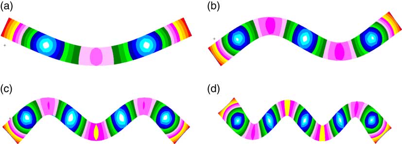
Figure 5 (Colour online) First four global bending mode shapes of the prototype. (a) 1st mode shape; (b) 2nd mode shape; (c) 3rd mode shape; (d) 4th mode shape.
Table 3 Natural frequency of prototype and the three-scaled models
As shown in Table 4, the similar deviations of each natural frequency of the three-scaled models are calculated according to the results shown in Table 3. The similar deviations are calculated as follows: the natural frequency of the scaled model is multiplied by the scale factor of frequency to obtain the predicted frequency of the scaled model for the prototype, then the predicted frequency and the frequency of the prototype are compared to calculate the error of similarity, that is,
 $$f_{{{\rm pre}}} {\equals}f_{{m}} \cdot {\rm \rlambda }_{f} ,{\rm {\varepsilon}{\equals}}\left| {{{f_{{{\rm pre}}} {\minus}f_{{{\rm pro}}} } \over {f_{{{\rm pro}}} }}} \right|{\times}100\%\,,$$
where the subscript ‘pre’ represents the predicted value of the scaled model for the prototype, and ε represents the error of similarity.
Table 4 The error of similarity for each natural frequency
From Table 4, it can be observed that the similar deviations of each natural frequency of the three-scaled models are not more than 1.03%. The results show that the deduced scaling laws in Equation (35) have a high degree of similarity, which can verify the equivalent similar method proposed in this paper. On the other hand, according to the special design of the three models, it is proved that the equivalent similar method can reach higher freedom in the design of the parameters such as thickness, number of stiffeners, cross-sectional shape and size of stiffeners, materials and so on.
5.0 CONCLUSIONS
The method to derive the scaling laws of the bending mode for the stiffened cylindrical shell is investigated. The limitation and similarity distortion of the scaling laws derived through traditional dimension analysis are discussed. The equivalent similar method is proposed to solve the problem and is applied to derive scaling laws of global bending mode for the stiffened cylindrical shell. The derived scaling laws are verified by the design and numerical analysis on a set of models including the prototype and the three-scaled models. The conclusions are drawn as follows:
(i) The result of similar deviations shows that the scaling laws derived from the equivalent similar method are highly accurate.
(ii) In the derived scaling laws, the terms relevant to the thickness of the cylindrical shell and the section size of the stiffener are reduced. Only the scaling laws between the cross-sectional area, the amount and the distribution of the stiffener are retained.
(iii) Compared to traditional similarity method, in the derived scaling laws, stiffeners in scaled model are no longer required to maintain the same amount and distribution as the prototype.
(iv) By the use of the derived scaling laws, stiffeners of scaled model can be designed with different cross-sectional shapes with that of the prototype.
As a consequence, the equivalent similar method proposed in this paper can solve some problems of similarity distortion and make the design of scaled model more freely. Moreover, the method can be applied to stiffened shells other than cylindrical shells and some complex structures with fine geometrical size, and thus provide theoretical basis for the related scaled model tests.
Acknowledgements
Authors sincerely acknowledge the support of College of Aerospace Science and Engineering, National University of Defense Technology, Hunan, China. This research was supported by the National Natural Science Foundation of China (grant no 11472003).