


NOMENCLATURE
- Φ, Θ, Ψ
-
body attitude angles
- Φ wind Ψ wind
-
wind incoming pitch and yaw angles
- Ψ R
-
rotor azimuth
- θ M 0, θ0 T
-
main and tail rotor collective angles
- θ1s , θ1c
-
main rotor cyclic angles
- A, B, C
-
matrices of the linear model
- F x F y F z
-
global forces at CG
- L M N
-
global moments at CG
- p, q, r
-
body rotation rates
- u, v, w
-
body velocities
- x e , y e , z e
-
body position in earth-fixed FoR
-
 $\vec{F}_i$
,
$\vec{F}_v$
$\vec{F}_i$
,
$\vec{F}_v$
-
inviscid and viscous fluxes
- R i, j, k
-
flux residuals at cell (i, j, k)
-
$\vec{S}$
-
source term
-
$\vec{u}_h$
-
local velocity in the rotor-fixed FoR
- V(t)
-
time dependent control volume
- w i, j, k
-
discretised conserved variables vector
-
$\vec{\mathbf {w}}$
-
conserved variables vector
- ρ
-
air density
-
$\vec{\omega }$
-
rotor rotational speed


1.0 INTRODUCTION
1.1 Background
State-of-the-art Computational Fluid Dynamics (CFD) methods and High-Performance Computing (HPC) facilities have advanced to the point where full helicopter configurations can be simulated with unprecedented levels of detail and good overall accuracy, even at challenging flight conditions(Reference Antoniadis, Drikakis, Zhong, Barakos, Steijl, Biava, Vigevano, Brocklehurst, Boelens, Dietz, Embacher and Khier1).
CFD has so far been used for a variety of problems: rotor/airframe and main/tail rotor interference, helicopter performance in hover and forward flight, rotor and airframe design, etc. The European project GOAHEAD is one of the efforts aimed at providing a high-quality database for validating CFD solvers. The experiments were conducted in the DNW low-speed facility(Reference Antoniadis, Drikakis, Zhong, Barakos, Steijl, Biava, Vigevano, Brocklehurst, Boelens, Dietz, Embacher and Khier1). Various flight conditions were simulated using a scaled model of a helicopter resembling the NH90, with a four-bladed main rotor and a two-bladed tail rotor. This case has since been used to validate numerous CFD codes(Reference Steijl and Barakos2-Reference Khier4).
Regardless of this progress, helicopters are versatile aircraft with capabilities extending beyond quasi-steady flight: rapid transition from hover to forward flight, and operations in confined areas are just some examples of manoeuvring flight. The Aeronautical Design Standard performance specification handling qualities requirements for military rotorcraft (ADS-33D-PRF) document provides guidelines on helicopter manoeuvring capabilities required for military operations. To date, any attempt to simulate ADS-33 cases has been performed with Blade-Element Momentum (BEM) or momentum theory models.
Ship/helicopter take-off/recovery operations – also referred to as the dynamic interface problem(Reference Zan5) – is a typical example of characterising the handling qualities of an aircraft. Expensive and time-consuming campaigns of at-sea trials are conducted to certify every aircraft/ship combination and define their operating limitations in terms of admissible wind strength and direction(Reference Hoencamp, Van Holten and Prasad6). Extensive experimental and numerical works have been carried out to reproduce the conditions of at-sea trials and expand the range of conditions investigated. Again, CFD efforts to simulate ship landing mainly use BEM tools coupled with some CFD input representing the ship wake. Such works include characterisation of ship wakes using numerical models(Reference Forrest and Owen7-Reference Thornber, Starr and Drikakis12), integration of the results into flight simulation environment(Reference Bunnell13-Reference Kaaria, Forrest, Owen and Padfield16), simultaneous ship/aircraft CFD simulations(Reference Polsky17,Reference Polsky18) , and attempts to couple CFD, flight dynamics, and pilot models to capture their interactional effects(Reference Alpman, Long, Bridges and Horn19-Reference Forsythe, Lynch, Polsky and Spalart23).
When it comes to experimental works, these include wind-tunnel measurements of the ship airwake(Reference Zan and Garry24-Reference Rosenfeld, Kimmel and Sydney27) and interaction between obstacles and rotor wakes(Reference Zan28-Reference Iboshi, Itoga, Prasad and Sankar37) as well as full-scale campaigns(Reference Snyder, Burks, Brownell, Luznik, Miklosovic, Golden, Hartsog, Lemaster, Roberson, Shishkoff, Stillman and Wilkinson38,Reference Snyder, Kang and Burks39) .
Simulating manoeuvring flight requires coupling CFD with flight mechanics methods and tracking or pilot models. With the problem of simulating the Dynamic Interface in mind, the relationships between the components of the simulation are shown in Fig. 1. The helicopter and ship aerodynamics and external disturbances can be modelled directly in the CFD solver, while the integrated loads can be passed on to flight mechanics methods to determine the helicopter position and attitude. Then, a tracking method or pilot model can be used to adjust the helicopter controls and follow a prescribed trajectory. The tracking can be optimal using minimisation methods, or it can be realistic, by modelling human behaviour. External information and sensory cues may be used by the pilot model, and it includes physiological and environmental feedbacks(Reference Mohammad and Cook40).
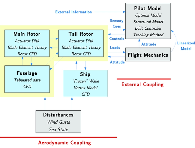
Figure 1. Description of the couplings associated with the simulation of the Dynamic Interface.
1.2 Past works
In this section, we are looking at work where CFD and flight mechanics are coupled. Such works are not common in the literature that is dominated by papers on CFD coupling with structural dynamics or multi-body dynamics within the general area of rotorcraft simulations. Ananthan et al(Reference Ananthan, Baeder, Sim, Hahn and Iaccarino41) interfaced the UMARC code with two CFD codes, OVERTURNS and SUmb, in a loosely coupled fashion and added acoustic predictions to the simulations of the SMART Rotor. Test cases included trailing-edge flaps and experimental data was collected by DARPA/NASA/Boeing/Army in 2008. Results showed good agreement, and their study focused primarily on noise prediction.
The case of the UTTAS pull-up manoeuvre is frequently reported in the literature(Reference Thomas, Ananthan and Baeder42-Reference Abhishek, Ananthan, Baeder and Chopra44). The manoeuvre was performed using an instrumented UH60 helicopter and is of great interest as it extends outside of the aircraft flight envelope. During the manoeuvre, the aircraft experiences up to 2.1 g acceleration with important stall events and transonic flow regions on the blades. In a key study from Bhagwat et al(Reference Bhagwat, Ormiston, Saberi and Xin43), the 40 revolutions of the UTTAS pull-up manoeuvre were analysed, in terms of blade loading, rotor hub forces and moments, blade flapping and lead-lag behaviour, push-rod and lag damper forces. The stand-alone RCAS code implementing a lifting line method with dynamic inflow model was compared with the coupled RCAS/OVERFLOW2 method. The coupled method consistently reduced the discrepancy with the experimental data, mainly due to the fact that it is a fast, highly loaded manoeuvre, with stalled and transonic flow regions that are poorly predicted using simpler aerodynamic models. However, it was noted that CFD did not always capture these effects and the improvements it offered may be more or less significant, depending on the flow conditions. Improving the CFD grid and the turbulence models employed were put forward as possible remedies. The paper concluded that quasi-steady simulations reproducing some specific instants of the manoeuvre offered good results at a much reduced computational cost. However, this was based on known flight conditions, derived directly from the experimental data, while the simulations were carried out for the main rotor only with the fuselage and tail rotor omitted. This simplification had consequences, especially on the prediction of blade flapping at peak loading.
Abhishek et al(Reference Abhishek, Ananthan, Baeder and Chopra44) also studied the UTTAS pull-up manoeuvre using the UMARC/OVERFLOW2 coupled CFD/CSD method by predicting blade deformations from measured airloads and using these deformations for analyses using lifting-line theory and CFD. The control angles were determined a priori using the lifting line method, in an iterative fashion, to obtain the forces and moments recorded during the campaign. The study focused on capturing dynamic stall events that occurred during the higher-loading phase of the manoeuvre. Interestingly, the CFD simulations were performed in a non-inertial frame of reference and therefore the inertial effects were added to the Navier Stokes equations as a source term. Sitaraman and his co-workers focussed on rotor load predictions during manoeuvres considering blade aeroelasticity but having prescribed flight paths(Reference J. Sitaraman45,Reference J. Sitaraman46) .
Masarati et al(Reference Masarati, Morandini and Mantegazza47) developed a multi-body dynamics framework designed to be interfaced with external aerodynamics and structural dynamics tools. The method found applications in rotorcraft studies for modelling pilot arm dynamics, and flapping wing fluid/structure coupling but has not yet been applied to helicopter rotor systems in manoeuvring flight.
Yu et al(Reference Yu, Wachspress, Saberi, Hasbun, Ho and Yeo48) combined the fast lifting surface method, free-wake and panel fuselage models of the CHARM tool with the deforming rotor system of RCAS. More accurate results were obtained using CHARM’s advanced methods over simple aerodynamic tables and lifting line theory for rotors in forward flight.
Beaumier et al(Reference Beaumier, Costes, Rodriguez, Poinot and Cantaloube49) and Servera et al(Reference Servera, Beaumier and Costes50) of ONERA coupled the HOST method with the CFD code elsA to include blade motion and aero-elasticity into the simulation. Results were compared against experimental data available for the 7A/7AD rotor. Weak ‘once-per-revolution’ and strong ‘once-per-time-step’ coupling methods were investigated. Similar results were reported in terms of rotor trim condition and the weak coupling was shown to converge more efficiently. However, it was noted that although the weak coupling method was good for periodic conditions, it was not appropriate for non-periodic cases like manoeuvers.
A similar method was implemented in the HMB solver coupling NASTRAN and HMB and Dehaeze and Barakos(Reference Dehaeze and Barakos51) also give an overview of the literature on CFD/CSD coupling. Results were limited to hovering rotors but showed reasonable agreement with the available experimental data.
Lee(Reference Lee and Horn20) studied the ship-helicopter interaction by performing one-way coupled calculations: the ship wake was calculated prior to the coupled analysis and loaded as a set of look-up tables into an analytical tool to simulate the unsteadiness of the ship wake. The method is similar to what is used in most flight-simulation environments as it uses of simplified models and lacks feedback from the rotor to the ship wake.
Bridges et al(Reference Bridges, Horn, Alpman and Long22) used the same approach but performed two-way calculations in which the information from the rotor loading was fed back to the CFD via the use of momentum source terms. Again, the rotor was simulated analytically and the method suffered from several simplifications. However, simulations included the use of a pilot model and the comparison of the results with a human-piloted maneuver showed similar variations of control history. Finally, works on taking CFD data to flight simulators are also found in the literature and the work of Forsythe(Reference Forsythe52) is just one of many examples.
1.3 Objectives of the current work
The present work demonstrates coupling of CFD and flight mechanics for simulation of manoeuvring rotorcraft and applies it to the case of ship/helicopter landing. The CFD method has been adapted to solve the Navier-Stokes equations directly in the inertial ‘earth-fixed’ frame of reference. The Helicopter Flight Mechanics solver (HFM) was also designed for the study of rotorcraft dynamics and includes a trimming algorithm and a pilot model. The underlying method and its implementation in HMB are described in this work. Aeroelastic effects on the rotor blades are neglected for simplicity, and to keep the CPU time requirements low, relatively coarse grids are used, to demonstrate the principles of the proposed method. The lack of experimental data for validation of coupled CFD flight mechanics simulations is also acknowledged. The following sections present elements of validation of the HMB solver for helicopters in forward-flight at low advance ratio and the prediction of ship wakes. Subsequently, a typical ship landing manoeuvre is split into three elements that serve as simpler tests for demonstrating the new coupled method. The paper finishes with conclusions and elements of future work.
2.0 NUMERICAL METHODS
2.1 Methodology for dynamic interface simulation
For this work, the stand-alone Helicopter Flight Mechanics (HFM) code was developed based on Blade Element Momentum (BEM) theory, a dynamic inflow model, and aerodynamic look-up tables. It was then integrated with the Helicopter Multi-Block (HMB) CFD solver(Reference Barakos, Steijl, Badcock and Brocklehurst53).
A versatile grid motion method was also implemented and the formulation of the CFD solver adapted to use an earth-fixed frame of reference, in addition to the wind-tunnel frame of reference used by most CFD solvers. Integrated loads and helicopter state information are passed between the flight mechanics and CFD solvers at every time step of the simulation. Spatial transformations are applied to account for the fact that HFM and HMB use different frames of reference. The integrated vehicle and component loads are also converted to dimensional values before being used in HFM, since all information stored by HMB is dimensionless.
HFM can run as a stand-alone code at a much reduced computational cost in comparison to CFD. The present methodology relies on the approximate models to generate the linear models of the aircraft necessary for the trimming and pilot control methods. Integrated aerodynamics loads from CFD are substituted directly to the approximate ones by HFM during re-trimming and simulated flight. Individual segments of a typical Royal Navy ship landing manoeuvre serve as test cases for simulating manoeuvring flight, using a Sea King helicopter geometry with five-bladed main and tail rotors. For shipborne manoeuvres, a simplified Halifax-class Frigate geometry is used, known in the literature as the Canadian Patrol Frigate (CPF)(Reference Lee and Zan31).
In the literature, various comprehensive codes are described such as HOST (Eurocopter), CAMRAD II (Johnson Aeronautics), MBDyn (Politecnico di Milano), UMARC (University of Maryland), CHARM/RCAS (US Army). They include blade aero-elasticity, advanced wake modelling, empirical corrections and their low computational cost allows for the simulation of complex flight condition, even in real time. However, some effects are only captured directly by CFD, like blade-vortex interaction, main/tail rotor interaction, main rotor/fuselage interaction, deep stall, etc.
When it comes to flight simulation, typically, analytical tools are used to predict the helicopter and rotor system states that are then used for CFD simulations, although consistency between the two results can be obtained only by coupling the methods. A large amount of work has been done in coupling CFD and analytical tools particularly for accurately predicting the rotor blade motion and deformation. Depending on the objective, different levels of coupling may be used. In the case of a weak/loose coupling in aeroelasticity, information is exchanged, usually every main rotor revolution. The concept of (very) strong/tight coupling requires that the two problems work with the same time-scales. Typically, data is exchanged at every time step or sub-step of the CFD solver, to ensure consistency between the solutions of the two methods. Weak coupling is sufficient to determine the trim state of a rotor system for a given flight condition but strongly coupled, time-accurate simulations are required if the system has no time-periodicity, such as during manoeuvres.
Rotorcraft blades are highly flexible and their deformations need to be taken into account using dedicated Computational Structural Dynamics (CSD) codes to accurately predict the aircraft performance. To achieve CFD/CSD coupling, a finite element model is built to match the blades structural properties. The increased complexity of the system usually leads to longer convergence time but the accuracy of the solution is greatly improved.
2.2 CFD solver
The HMB code(Reference Barakos, Steijl, Badcock and Brocklehurst53) was used for solving the flow around different ship and rotor geometries. HMB is a Navier-Stokes solver employing multi-block structured grids. For rotor flows, a typical multi-block topology used with HMB is described in Steijl et al(Reference Steijl, Barakos and Badcock54). A C-mesh is used around the blade and this is included in a larger H structure that fills up the rest of the computational domain. For parallel computations, blocks are shared amongst processors and communicate using a message-passing paradigm.
HMB solves the Navier-Stokes equations in integral form using the Arbitrary Lagrangian Eulerian (ALE) formulation for time-dependent domains with moving boundaries:
 $$\begin{equation}
\frac{d}{dt} \int _{V(t)} \vec{\mathbf {w}} dV + \int _{\partial V(t)} \left( \vec{F_i} \left(\vec{\mathbf {w}} \right) - \vec{F}_v \left( \vec{\mathbf {w}} \right) \right) \vec{(}n) dS = \vec{S},
\end{equation}$$
$$\begin{equation}
\frac{d}{dt} \int _{V(t)} \vec{\mathbf {w}} dV + \int _{\partial V(t)} \left( \vec{F_i} \left(\vec{\mathbf {w}} \right) - \vec{F}_v \left( \vec{\mathbf {w}} \right) \right) \vec{(}n) dS = \vec{S},
\end{equation}$$
where V(t) is the time-dependent control volume, ∂V(t) its boundary, and
 $\vec{\mathbf {w}}$
is the vector of conserved variables [ρ, ρu, ρv, ρw, ρE]
T
.
$\vec{\mathbf {w}}$
is the vector of conserved variables [ρ, ρu, ρv, ρw, ρE]
T
.
 $\vec{F}_i$
and
$\vec{F}_i$
and
 $\vec{F}_v$
are the inviscid and viscous fluxes, including the effects of the time-dependent, moving, computational domain.
$\vec{F}_v$
are the inviscid and viscous fluxes, including the effects of the time-dependent, moving, computational domain.
The Navier-Stokes equations are discretised using a cell-centred finite-volume approach on multi-block grids, leading to the following equation:
 $$\begin{equation}
\frac{\partial }{\partial t} \left( \mathbf {w}_{i,j,k} V_{i,j,k}\right) = -\mathbf {R}_{i,j,k} \left( \mathbf {w}_{i,j,k} \right),
\end{equation}$$
$$\begin{equation}
\frac{\partial }{\partial t} \left( \mathbf {w}_{i,j,k} V_{i,j,k}\right) = -\mathbf {R}_{i,j,k} \left( \mathbf {w}_{i,j,k} \right),
\end{equation}$$
where w represents the cell variables and R the residuals. i, j, and k are the cell indices and V i, j, k is the cell volume. Osher’s(Reference Osher and Chakravarthy55) scheme is used to discretise the convective terms and MUSCL variable interpolation is used to provide up to third order accuracy. The Van Albada limiter is used to reduce the oscillations near steep gradients. Viscous fluxes are treated with a second-order, central scheme. Temporal integration is performed using an implicit dual-time stepping method. The linearised system is solved using the generalised conjugate gradient method with a block incomplete lower-upper (BILU) pre-conditioner(Reference Axelsson56).
2.3 CFD grids
A total of three cases have been used to validate the HMB solver. The SFS2 ship was first meshed using three mesh densities for a sensitivity study, the finest being around 15 m cells. The GOAHEAD helicopter model contained a total of 90 m cells, including four-bladed main and two-bladed tail rotors, with attention paid to the region of the flow between the rotor and the tail plane and in the near wake, to capture as accurately as possible the shed vortices. No mesh convergence study was made for the GOAHEAD case though the employed mesh is finer than what was used for this case in one of our earlier investigations(Reference Steijl and Barakos2). Finally, eight structured, multi-block grids were used for the landing case, including four components: Sea King helicopter fuselage, main and tail rotor, and Canadian Patrol Frigate (CPF). The helicopter fuselage was split in three sections to ease the meshing process; the three elements and the two five-bladed rotors are interfaced using sliding planes. The total number of cells reached 23.5 m for the complete helicopter grid. This is coarser than what was used for the GOAHEAD case but the size was dictated by the required CPU time for computations. Especially for this case, where long computations of manoeuvres were envisaged, the employed parallel computer cluster did not have the capacity to deliver timely results with a finer mesh. A background grid was created to extend the computational domain when the helicopter was computed in isolation. The ship mesh and its background contain a total of 31 m cells. Figure 2 shows the mesh near the heli-deck for the CPF case. Figure 3 shows the mesh around the helicopter. The detailed count of the number of blocks and cells in each grid is given in Table 1.

Figure 2. Detail of the mesh above the Canadian Patrol Frigate heli-deck.

Figure 3. CFD mesh of the Sea King helicopter.
Table 1 Size of the meshes used for this work,1 simple frigate shape geometry,2 Sea King helicopter,3 Canadian patrol frigate geometry

2.4 Wind-tunnel versus earth-fixed frames of reference
The usual approach for CFD simulations consists in choosing a wind-tunnel frame of reference, keeping the aircraft fuselage and rotor axis of rotation fixed. The far-field velocity is uniform and dimensionless with U
∞ = 1, the advance ratio is typically set by applying a non-dimensional rotational speed of
 $\frac{1}{\mu R}$
on the rotor mesh.
$\frac{1}{\mu R}$
on the rotor mesh.
This approach is not appropriate for manoeuvring flight as the aircraft is free to translate and rotate in all 6 directions. All simulations were then performed in an ‘earth-fixed’ frame of reference. Since this is also an inertial frame of reference, no acceleration terms need to be added to the Navier-Stokes equations.
The dimensionless rotational speed of the rotor becomes
 $\frac{1}{R}$
and the advance ratios in each direction are then applied through the mesh velocity. The different formulations are summarised in Table 2. The table also includes the corresponding dimensional values used by the flight-mechanics solver.
$\frac{1}{R}$
and the advance ratios in each direction are then applied through the mesh velocity. The different formulations are summarised in Table 2. The table also includes the corresponding dimensional values used by the flight-mechanics solver.
Table 2 Definitions and correspondence between HFM and HMB codes

To demonstrate the validity of using the earth-fixed frame of reference and the new grid motion approach, the ONERA non-lifting rotor(Reference J-J Philippe and Chattot57) was used with an advance ratio of μ = 0.5. Figure 4 shows pressure contours on the blades at different azimuths obtained from the two techniques. There is no visible difference between the two sets of results, and the pressure everywhere on the blades agrees to the third significant digit or better.

Figure 4. ONERA non-lifting rotor in forward flight computed using two frames of reference.
2.5 Moving mesh method
A new moving mesh method had to be implemented to allow the relative motion of any grid with respect to another. One or several grids are defined in the absolute frame of reference, and subsequent grids are hierarchised by referring to a parent grid previously defined. The various grids are interfaced using either sliding plane boundaries, the chimera method, or both simultaneously. The rotors are treated separately as they require mesh deformation to allow for pitching and flapping motions, and possibly elastic blade deformations(Reference Steijl, Barakos and Badcock54,Reference Steijl and Barakos58) .
In this work, the most complex case is the manoeuvring Sea King above the ship deck. The absolute frame of reference contains the ship and fuselage grid that are allowed to move independently using the chimera method, the main and tail rotors are added, with the fuselage being their parent component. The transformations of each element are calculated at each time step. These put the mesh components to their reference position, calculate the loads on each element and position the grids for the next time step. The x-y-z convention is used for the rotation of every component except the blades that articulate according to their hinge order.
3.0 HELICOPTER FLIGHT MECHANICS
3.1 Flight mechanics method
The Helicopter Flight Mechanics (HFM) method is purpose-built for rotorcraft applications. A structural model gives a description of the aircraft and the relationship between the different components. The fuselage, tail plane and fin are assimilated to singular points where the forces and moments are applied. The fin and tail plane are weightless but contribute separately to the budget of loads.
With the forces and moments written at the center of gravity and the action of gravity added explicitly, the Euler’s equations of motion read as follows:
 $$\begin{equation}
&&\left\lbrace\begin{array}{ll}
\dot{u} = v\,\, r - q\,\, w + \frac{{\rm F}_{\rm x}}{{\rm M}} - {\rm g}\,\, \sin \theta \\[6pt]
\dot{v} = w\,\, p - u\,\, r + \frac{{\rm F}_{\rm y}}{{\rm M}} + {\rm g}\,\, \cos \theta\,\, \sin \phi, \\[6pt]
\dot{w} = u\,\, q - v\,\, p + \frac{{\rm F}_{\rm z}}{{\rm M}} + {\rm g}\,\, \cos \theta\,\, \cos \phi
\end{array}\right.
\end{equation}$$\\
$$\begin{equation}
&&\left\lbrace\begin{array}{ll}
\dot{u} = v\,\, r - q\,\, w + \frac{{\rm F}_{\rm x}}{{\rm M}} - {\rm g}\,\, \sin \theta \\[6pt]
\dot{v} = w\,\, p - u\,\, r + \frac{{\rm F}_{\rm y}}{{\rm M}} + {\rm g}\,\, \cos \theta\,\, \sin \phi, \\[6pt]
\dot{w} = u\,\, q - v\,\, p + \frac{{\rm F}_{\rm z}}{{\rm M}} + {\rm g}\,\, \cos \theta\,\, \cos \phi
\end{array}\right.
\end{equation}$$\\
 $$\begin{equation}
&&\left\lbrace \begin{array}{@{}l@{\quad }ll@{}}
{\rm I}_{xx} \dot{p} = {\rm I}_{xy}\,\, p\,\, r + ({\rm I}_{yy} - {\rm I}_{zz})\,\, q\,\, r + {\rm I}_{yz}\,\, (r^2 + q^2) + {\rm I}_{xz}\,\, p\,\, q + {\rm L}\\[6pt]
{\rm I}_{yy} \dot{q} = {\rm I}_{yz}\,\, p\,\, q + ({\rm I}_{zz} - {\rm I}_{xx})\,\, r\,\, p + {\rm I}_{xz}\,\, (p^2 - r^2) + {\rm I}_{xy}\,\, q\,\, r + {\rm M},\\[6pt]
{\rm I}_{zz} \dot{r} = {\rm I}_{xz}\,\, q\,\, r + ({\rm I}_{xx} - {\rm I}_{yy})\,\, p\,\, q + {\rm I}_{xy}\,\, (q^2 - p^2) + {\rm I}_{yz}\,\, p\,\, r + {\rm N} \end{array}\right.
\end{equation}$$
$$\begin{equation}
&&\left\lbrace \begin{array}{@{}l@{\quad }ll@{}}
{\rm I}_{xx} \dot{p} = {\rm I}_{xy}\,\, p\,\, r + ({\rm I}_{yy} - {\rm I}_{zz})\,\, q\,\, r + {\rm I}_{yz}\,\, (r^2 + q^2) + {\rm I}_{xz}\,\, p\,\, q + {\rm L}\\[6pt]
{\rm I}_{yy} \dot{q} = {\rm I}_{yz}\,\, p\,\, q + ({\rm I}_{zz} - {\rm I}_{xx})\,\, r\,\, p + {\rm I}_{xz}\,\, (p^2 - r^2) + {\rm I}_{xy}\,\, q\,\, r + {\rm M},\\[6pt]
{\rm I}_{zz} \dot{r} = {\rm I}_{xz}\,\, q\,\, r + ({\rm I}_{xx} - {\rm I}_{yy})\,\, p\,\, q + {\rm I}_{xy}\,\, (q^2 - p^2) + {\rm I}_{yz}\,\, p\,\, r + {\rm N} \end{array}\right.
\end{equation}$$
Data is tabulated for a range of Reynolds and Mach numbers and interpolated at the local flow conditions. The Blade Element Momentum (BEM) method is used for the rotors. Each blade is typically split in 20 elements, each approximated to a 2D section and loads are calculated as functions of the Reynolds and Mach numbers. Alternatively, if the model is used with the CFD solver, forces and moments are computed on-the-fly by integrating over all surfaces of the helicopter (rotors, fuselage, etc.) and passing the data directly at each step of the simulation.
To complete the BEM, the three-state dynamic inflow model by Peter and He(Reference Peters and He59) is implemented to calculate the component of inflow velocity through the rotor disk. The inflow model and blade aerodynamics, in particular, use first-order approximations and a set of look-up tables, and do not take into account the 3D and unsteady effects typical of rotor blades.
For this study, The MK50 Sea King helicopter was chosen. It is a medium-lift transport and utility helicopter designed and widely used for maritime operations, capable of carrying up to 28 troops for a maximum take off weight of about 9,700 kg. Information about the MK50 model can be found in a series of DTIC reports(Reference Arney and Gilbert60-Reference Feik and Perrin62). The main characteristics of the aircraft are collected in Table 3.
Table 3 Characteristics of the Sea King MK50 helicopter(Reference Arney and Gilbert60-Reference Feik and Perrin62)

Table 4 List of the GOAHEAD test cases with corresponding flow conditions (Reproduced from Antoniadis et al(Reference Antoniadis, Drikakis, Zhong, Barakos, Steijl, Biava, Vigevano, Brocklehurst, Boelens, Dietz, Embacher and Khier1))

Trimming the helicopter consists in finding the appropriate pilot inputs to maintain straight and level flight. The method builds a Jacobian matrix (Equation (5)) from a chosen set of parameters (Equation (6)) and variables (Equation (7)) and uses this matrix to find the values of the pilot inputs that will minimise forces and moments on the helicopter. The four pilot inputs and two body attitude angles are chosen as parameters to obtain a system of six equations and six dependant variables:
 $$\begin{equation}
{{\bm J}} &=& \left(\frac{d {{\bm f}}_i}{d x_j}\right)_{i,j},
\end{equation}$$\\
$$\begin{equation}
{{\bm J}} &=& \left(\frac{d {{\bm f}}_i}{d x_j}\right)_{i,j},
\end{equation}$$\\
 $$\begin{equation}
{{\bm x}}&=& (\theta _{\rm 0}^{\rm M}\,\, \theta _{\rm 1c}\,\, \theta _{\rm 1s}\,\, \Theta\,\, \Phi\,\, \theta _{\rm 0}^{\rm T})^{\rm T}, \\
\end{equation}$$
$$\begin{equation}
{{\bm x}}&=& (\theta _{\rm 0}^{\rm M}\,\, \theta _{\rm 1c}\,\, \theta _{\rm 1s}\,\, \Theta\,\, \Phi\,\, \theta _{\rm 0}^{\rm T})^{\rm T}, \\
\end{equation}$$
 $$\begin{equation}
{{\bm f}}&=& (F_{\rm X}\,\, F_{\rm Y}\,\, F_{\rm Z}\,\, L\,\, M\,\, N)^{\rm T}.
\end{equation}$$
$$\begin{equation}
{{\bm f}}&=& (F_{\rm X}\,\, F_{\rm Y}\,\, F_{\rm Z}\,\, L\,\, M\,\, N)^{\rm T}.
\end{equation}$$
 $\delta {{\bm x}}$
so the calculated forces
$\delta {{\bm x}}$
so the calculated forces
 $\delta {{\bm f}}$
are minimised:
$\delta {{\bm f}}$
are minimised:
 $$\begin{equation}
\delta {{\bm x}}= {{\bm J}}^{-1} \delta {{\bm f}}.
\end{equation}$$
$$\begin{equation}
\delta {{\bm x}}= {{\bm J}}^{-1} \delta {{\bm f}}.
\end{equation}$$
The matrix is recalculated before each iteration to increase stability and convergence speed. A second trimming method has been implemented in HMB/HFM, referred to as hybrid trimming: it uses a reduced system of four equations, where the parameters Θ and Φ are frozen to the previously calculated value, and replaces the loads by the ones obtained in the CFD. The reduced Jacobian is calculated around the previous trim state using the same method as before, with the following variables/parameters:
 $$\begin{equation}
{{\bm x}} &=& (\theta _{\rm 0}^{\rm M}\,\, \theta _{\rm 1c}\,\, \theta _{\rm 1s}\,\, \theta _{\rm 0}^{\rm T})^{\rm T},
\end{equation}$$\\
$$\begin{equation}
{{\bm x}} &=& (\theta _{\rm 0}^{\rm M}\,\, \theta _{\rm 1c}\,\, \theta _{\rm 1s}\,\, \theta _{\rm 0}^{\rm T})^{\rm T},
\end{equation}$$\\
 $$\begin{equation}
{{\bm f}}&=& (F_{\rm Z}\,\, L\,\, M\,\, N)^{\rm T}.
\end{equation}$$
$$\begin{equation}
{{\bm f}}&=& (F_{\rm Z}\,\, L\,\, M\,\, N)^{\rm T}.
\end{equation}$$
Once straight and level flight is achieved, it is possible to begin the simulation of manoeuvring flight.
3.2 Manoeuvring flight
During a manoeuvre, the aircraft is out-of-trim and the global loads applied to the system are not null, furthermore the pilot controls must be in accordance with the objective of the manoeuvre, typically following a predetermined flight path.
To simulate manoeuvring helicopters, controllers were developed and designed to be representative of the behaviour of a real pilot. The SYCOS method has been widely used in the past(Reference Bradley and Brindley63,Reference Thomson and Bradley64) and is based on an inverse model of the aircraft which consists of a set of matrices that allow to compute pilot inputs from a determined flight path. The model is linear and can be solved analytically for simple cases. The SYCOS method uses an approximate linear inverse model along with a correction method that modifies the problem depending on how accurately the helicopter is following the pre-determined flight path. The SYCOS method proved to be suitable for simulating standard maneuvers described in the ADS33 documentation such as a slalom(Reference Thomson and Bradley64).
To provide good control and trajectory tracking performance for more complex helicopter models, more advanced methods are needed. The Linear-Quadratic Regulator(Reference Kwakernaak65) is an example of a widely used control method based on least-squares minimisation. It uses a full linear model of the aircraft to provide control estimates during a manoeuvre, given a prescribed trajectory. The inverse modelling method is presented here as it permits to a priori estimate the pilot controls but the LQR method was applied for piloted simulations, with or without CFD.
A typical formulation used for inverse modelling is
 $$\begin{equation}
\skew4\dot{{{\bm x}}}= A{{\bm x}}+ B{{\bm u}},
\end{equation}$$
$$\begin{equation}
\skew4\dot{{{\bm x}}}= A{{\bm x}}+ B{{\bm u}},
\end{equation}$$
where
 ${{\bm x}}$
and
${{\bm x}}$
and
 ${{\bm u}}$
are the state and control vectors, respectively:
${{\bm u}}$
are the state and control vectors, respectively:
 $$\begin{equation}
{{\bm x}}&=& (u\,\, v\,\, w\,\, p\,\, q\,\, r\,\, \Phi\,\, \Theta\,\, \Psi ),
\end{equation}$$\\
$$\begin{equation}
{{\bm x}}&=& (u\,\, v\,\, w\,\, p\,\, q\,\, r\,\, \Phi\,\, \Theta\,\, \Psi ),
\end{equation}$$\\
 $$\begin{equation}
{{\bm u}} &=& (\theta ^{\rm M}_{\rm 0}\,\, \theta _{\rm 1c}\,\, \theta _{\rm 1s}\,\, \theta ^{\rm T}_{\rm 0}).
\end{equation}$$
$$\begin{equation}
{{\bm u}} &=& (\theta ^{\rm M}_{\rm 0}\,\, \theta _{\rm 1c}\,\, \theta _{\rm 1s}\,\, \theta ^{\rm T}_{\rm 0}).
\end{equation}$$
 $$\begin{equation}
{{\bm y}}= C {{\bm x}}.
\end{equation}$$
$$\begin{equation}
{{\bm y}}= C {{\bm x}}.
\end{equation}$$
The role of the matrix C is to select a set of variables and reduce the system so A becomes square. The number of parameters is usually four; if the earth-based components of velocity and the heading angle are prescribed, the output vector y is
 $$\begin{equation}
{{\bm y}}= (u_{\rm e}\,\, v_{\rm e}\,\, w_{\rm e}\,\, \Psi ),
\end{equation}$$
$$\begin{equation}
{{\bm y}}= (u_{\rm e}\,\, v_{\rm e}\,\, w_{\rm e}\,\, \Psi ),
\end{equation}$$
where the subscript e refers to quantities given in the earth-bound frame of reference.
Pilot controls come directly from prescribing
 ${{\bm y}}^*$
in the inverse problem:
${{\bm y}}^*$
in the inverse problem:
 $$\begin{equation}
{{\bm u}}^* = (CB)^{-1} (\dot{{{\bm y}}}^* - C A {{\bm x}}).
\end{equation}$$
$$\begin{equation}
{{\bm u}}^* = (CB)^{-1} (\dot{{{\bm y}}}^* - C A {{\bm x}}).
\end{equation}$$
By prescribing y*, the inverse modelling method allows to predict the pilot controls required to follow the trajectory (u*).
The LQR method(Reference Kwakernaak65) is based on a full linear model of the aircraft, where the state space and control vectors are modified so
 $$\begin{equation}
{{\bm x}}&=& \left( u\,\, v\,\, w\,\, p\,\, q\,\, r\,\, x_{\rm e}\,\, y_{\rm e}\,\, z_{\rm e}\,\, \Phi\,\, \Theta\,\, \Psi \right),
\end{equation}$$\\
$$\begin{equation}
{{\bm x}}&=& \left( u\,\, v\,\, w\,\, p\,\, q\,\, r\,\, x_{\rm e}\,\, y_{\rm e}\,\, z_{\rm e}\,\, \Phi\,\, \Theta\,\, \Psi \right),
\end{equation}$$\\
 $$\begin{equation}
{{\bm u}} &=& \left( \theta ^{\rm M}_{\rm 0}\,\, \theta _{\rm 1c}\,\, \theta _{\rm 1s}\,\, \theta ^{\rm T}_{\rm 0} \right),
\end{equation}$$
$$\begin{equation}
{{\bm u}} &=& \left( \theta ^{\rm M}_{\rm 0}\,\, \theta _{\rm 1c}\,\, \theta _{\rm 1s}\,\, \theta ^{\rm T}_{\rm 0} \right),
\end{equation}$$
 $({{\bm x}}^*,{{\bm u}}^*)$
as
$({{\bm x}}^*,{{\bm u}}^*)$
as
 $$\begin{equation}
\delta \skew4\dot{{{\bm x}}}= A^* \delta {{\bm x}}+ B^* \delta {{\bm u}},
\end{equation}$$
$$\begin{equation}
\delta \skew4\dot{{{\bm x}}}= A^* \delta {{\bm x}}+ B^* \delta {{\bm u}},
\end{equation}$$
where matrices A* and B* are the linear approximation of the aircraft around a particular trim point.
The nonlinear function
 ${{\bm f}}({{\bm x}},{{\bm u}})$
describes the evolution of the state space vector from the trim state
${{\bm f}}({{\bm x}},{{\bm u}})$
describes the evolution of the state space vector from the trim state
 ${{\bm x}}^*$
to the state
${{\bm x}}^*$
to the state
 ${{\bm x}}$
under the action of the fixed input
${{\bm x}}$
under the action of the fixed input
 ${{\bm u}}$
and is computed by integrating Equation (19) over several revolutions of the rotor to let the flapping motion transient be sufficiently damped.
${{\bm u}}$
and is computed by integrating Equation (19) over several revolutions of the rotor to let the flapping motion transient be sufficiently damped.
The aim of the autopilot is to control the position (x
e, y
e, z
e) of the helicopter in the earth reference frame and its heading Ψ. We recast this trajectory tracking problem into the LQR setting as follows. At each time instant, we consider the closest trimmed condition of the helicopter and compute the associated linearised model. Then, if
 $\delta {{\bm x}}$
is the deviation of the state vector from the desired state, the variation
$\delta {{\bm x}}$
is the deviation of the state vector from the desired state, the variation
 $\delta {{\bm u}}$
of the controls is determined as the LQR optimal feedback due to the deviation
$\delta {{\bm u}}$
of the controls is determined as the LQR optimal feedback due to the deviation
 $\delta {{\bm x}}$
. The LQR controller will in fact drive
$\delta {{\bm x}}$
. The LQR controller will in fact drive
 $\delta {{\bm x}}$
to zero by minimising the quadratic cost function:
$\delta {{\bm x}}$
to zero by minimising the quadratic cost function:
 $$\begin{equation}
J = \int _0^\infty \left(\delta {{\bm x}}^{\rm T} Q \delta {{\bm x}}+ \delta {{\bm u}}^{\rm T} R \delta {{\bm u}}\right) {\rm d} t,
\end{equation}$$
$$\begin{equation}
J = \int _0^\infty \left(\delta {{\bm x}}^{\rm T} Q \delta {{\bm x}}+ \delta {{\bm u}}^{\rm T} R \delta {{\bm u}}\right) {\rm d} t,
\end{equation}$$
where Q and R are weighting matrices that define the ‘importance’ of the the states and of the controls in the cost function. The solution to the minimisation problem is
 $$\begin{equation}
\delta {{\bm u}}_{\rm LQR} = - K \delta {{\bm x}},
\end{equation}$$
$$\begin{equation}
\delta {{\bm u}}_{\rm LQR} = - K \delta {{\bm x}},
\end{equation}$$
where K is the optimal feedback matrix given by
 $$\begin{equation}
K = R^{-1} B^{\rm T} P,
\end{equation}$$
$$\begin{equation}
K = R^{-1} B^{\rm T} P,
\end{equation}$$
and P is the solution of the continuous algebraic Riccati equation:
 $$\begin{equation}
A^{\rm T} P + P A - P B R^{-1} B^{\rm T} P + Q = 0.
\end{equation}$$
$$\begin{equation}
A^{\rm T} P + P A - P B R^{-1} B^{\rm T} P + Q = 0.
\end{equation}$$
As can be seen, the optimal LQR feedback matrix K does not depend on the solution and may therefore be calculated prior to the simulation for the various representative trim states. To achieve better tracking performance the LQR controller has been augmented with a simple PI controller:
 $$\begin{equation}
\delta {{\bm u}}_{\rm PI}&=&-{\rm diag}(K^{\rm P}_1\,\, K^{\rm P}_2\,\, K^{\rm P}_3\,\, K^{\rm P}_4 ) {{\bf e}}
\end{equation}$$\\
$$\begin{equation}
\delta {{\bm u}}_{\rm PI}&=&-{\rm diag}(K^{\rm P}_1\,\, K^{\rm P}_2\,\, K^{\rm P}_3\,\, K^{\rm P}_4 ) {{\bf e}}
\end{equation}$$\\
 $$\begin{equation}
&&-{\rm diag}(K^{\rm I}_1\,\, K^{\rm I}_2\,\, K^{\rm I}_3\,\, K^{\rm I}_4 ) \int _{t-\Delta t}^{t} {{\bf e}}~ {\rm d}t,
\end{equation}$$
$$\begin{equation}
&&-{\rm diag}(K^{\rm I}_1\,\, K^{\rm I}_2\,\, K^{\rm I}_3\,\, K^{\rm I}_4 ) \int _{t-\Delta t}^{t} {{\bf e}}~ {\rm d}t,
\end{equation}$$
 $$\begin{equation}
{{\bf e}}= \left\lbrace \begin{array}{c}{{\bm x}}_{\rm e} - \skew4\hat{{{\bm x}}}_{\rm e}\\
\Psi - \hat{\Psi }\end{array} \right\rbrace ,
\end{equation}$$
$$\begin{equation}
{{\bf e}}= \left\lbrace \begin{array}{c}{{\bm x}}_{\rm e} - \skew4\hat{{{\bm x}}}_{\rm e}\\
\Psi - \hat{\Psi }\end{array} \right\rbrace ,
\end{equation}$$
and
 ${{\bm x}}_{\rm e}$
and
${{\bm x}}_{\rm e}$
and
 $\skew4\hat{{{\bm x}}}_{\rm e}$
are the actual and desired trajectory in Earth reference frame, respectively, and Ψ and
$\skew4\hat{{{\bm x}}}_{\rm e}$
are the actual and desired trajectory in Earth reference frame, respectively, and Ψ and
 $\hat{\Psi }$
are the actual and desired heading, respectively. The coefficients K
P
i
and K
I
i
(i = 1, . . ., 4) are, respectively, the proportional and integral gains. Their values were adjusted so the response of the aircraft to simple control inputs is not oscillatory.
$\hat{\Psi }$
are the actual and desired heading, respectively. The coefficients K
P
i
and K
I
i
(i = 1, . . ., 4) are, respectively, the proportional and integral gains. Their values were adjusted so the response of the aircraft to simple control inputs is not oscillatory.
The value of the control angles at each time instant is therefore given by their value in the reference trimmed condition plus the feedback given by the LQR and PI controllers:
 $$\begin{equation}
{{\bm u}}= {{\bm u}}^* + \delta {{\bm u}}_{\rm LQR} + \delta {{\bm u}}_{\rm PI}.
\end{equation}$$
$$\begin{equation}
{{\bm u}}= {{\bm u}}^* + \delta {{\bm u}}_{\rm LQR} + \delta {{\bm u}}_{\rm PI}.
\end{equation}$$
3.3 Time-line of a full simulation
Ship wake prediction and rotor simulations are two different problems and involve different reference time scales and Mach and Reynolds numbers. Simulations of the isolated ship wakes showed(Reference Crozon, Steijl and Barakos66) that 100 time steps per beam travel time are usually enough to capture the unsteady characteristics of the wake, while rotor simulations are usually performed with 0.25 to 1° of rotor azimuth per step, the ratio between the two time steps being somewhere between 10 and 100.
Prior to the simulation, the ship flowfield is calculated using a time step suitable for the ship wake to eliminate the transient flow and reach a converged state (in the statistical sense). The helicopter is then included in the simulation so the wake of the fuselage is also taken into account. However, the rotor is fixed, since the time step chosen corresponds to about 12° of azimuthal resolution for the main rotor – 60° for the tail rotor – and would likely cause the simulation to diverge.
The coupled simulation is then started and follows the steps of Fig. 5. Important decisions about the use of the trimmer, or if a trimmed simulation is needed are taken early in the process, and similarly the selection of linearised models for the flight mechanics of the aircraft is decided before time-marching with CFD computations. The converged flow solution is used but a smaller time step is employed that allows to spin the two rotors. Again, the simulation is left to run for about five revolutions of the main rotor to allow the rotor wake to clear the airframe and reach a converged state. The loads on the rotor should be reasonably similar from one revolution to the next but are subject to variations caused by the ship wake.

Figure 5. Timeline of manoeuvring flight simulation.
The helicopter uses a trim state that was determined in free air and re-trimming is not attempted, since the flow is now constantly varying. Instead, the residual forces and moments are cancelled out at the beginning of the manoeuvre to approximate trimmed flight.
Finally, the fully coupled simulations of the shipborne manoeuvre is started. The body is frozen in space for a short period of time at the beginning of the simulation to cancel the residual loads and start feeding data into the LQR method. The aircraft is then free to move in all directions and the LQR tracking method is immediately activated to provide pilot controls.
4.0 VALIDATION WORK
CFD-based Dynamic Interface simulations require the solver to perform well across a wide range of flow conditions, including low-speed, slow flow at very high Reynolds number around the ship and fuselage, and high-speed flows around the rotor blades. Validation of the HMB solver was therefore carried out using the SFS2 ship geometry(Reference Cheney and Zan67) and the GOAHEAD database(Reference Boelens68) to cover ship wakes and complete helicopters.
4.1 Validation for ship airwake
The sharp edges typical of most ship geometries fix the points of separation in the flow and generate large zones of recirculation in the vicinity of the ship superstructure. The wake is typically unsteady, with shedding frequencies in the range of 0.2–2 Hz depending on the size of the elements of the superstructure and the wind speed. The Reynolds number based on the ship length is around 100 m for a frigate while the Mach number is below 0.1.
A campaign of measurements was conducted at the Naval Surface Warfare Center Carderock Division (NSWCCD)(Reference Quon, Cross, J., C. and R.26,Reference Rosenfeld, Kimmel and Sydney27) . Published results include mean values of streamwise velocity, local flow pitch and yaw angle along eight vertical lines positioned in the direct vicinity of the ship, above the landing deck (Fig. 6). Experiments were conducted at 0° and 60° wind angle.

Figure 6. Position of the eight vertical probe lines, from Quon and Rosenfeld(Reference Quon, Cross, J., C. and R.26,Reference Rosenfeld, Kimmel and Sydney27) .
The numerical simulations reproduced the two experimental conditions using Detached Eddy Simulation with the Spalart-Allmaras turbulence model (DES-SA)(Reference Spalart, Deck, Shur, Squires, Strelets and Travin69) and the Scale-Adaptive Simulation (SAS)(Reference Menter and Egorov70). Results for each of the two wind angles have a similar level of agreement and only the 60° case is shown in this paper.
A grid sensitivity study was conducted using the DES-SA model and the finer grid was used for production runs. Figures 7 and 8 show the results obtained using the DES-SA and SAS models respectively. The agreement between experimental and CFD data is good for both models. The DES-SA results show that the recirculation zone is over-predicted by the CFD, with some deficits of velocity, and some discrepancies in terms of the downwash angle (pitch).

Figure 7. Time-averaged values of velocity and flow angles along 8 vertical lines. DES-SA model, WOD = 60°, Re = 6.58 × 10⁵.

Figure 8. Time-averaged values of velocity and flow angles along eight vertical lines. SAS model, WOD = 60°, Re = 6.58 × 10⁵.
Unsteady results are reproduced in Fig. 9. No experimental data has been published to help estimate the level of unsteadiness in the flow for this particular geometry. Simulations using DES show that a fine grid containing 15 m cells was required to capture a level of unsteadiness similar to levels reported with in situ measurements. Mora(Reference Mora71) reported a turbulence intensity of about 25% behind a scaled frigate in a wind tunnel. The frequency analysis in (a) and (b) show that similar levels of unsteadiness are found when using the SAS model with the intermediate and fine grid densities.

Figure 9. Comparison of URANS, DES-SA, and SAS models and grid density study. Headwind case, Re = 6.58 × 10⁵.
At the given flow condition, a clear dominant shedding frequency is found at 0.35 Hz, which is within the 0.2–2 Hz range typical of ship airwakes(Reference Zan, Syms and Cheney72). In the region of higher frequencies, it is found that all grids capture well the −5/3 slope that characterises the Kolmogorov scale with the exception of the SAS model on the fine grid, mainly due to the short length of the available computed signal. The finer grid was used for the rest of the ship wake study and the results were averaged in time from the unsteady solutions and over a converged and significant period of time. However, for the coupled simulations of the manoeuvring helicopter in the wake of the ship, the SAS model was used as the grid density is closer to the intermediate one and it is a numerically more robust model than the DES-SA. Considering that the SAS model performs well, that is numerically stable, and that it maintain a reasonable level of unsteadiness in coarser regions of the grid, it will be preferred over the DES model in the rest of the study when a ship wake is present.
4.2 Validation for helicopter configuration
The low-speed case termed Test case 2 or ‘TC2’ of the GOAHEAD database(Reference Antoniadis, Drikakis, Zhong, Barakos, Steijl, Biava, Vigevano, Brocklehurst, Boelens, Dietz, Embacher and Khier1) is used to validate HMB for helicopter configurations at low advance ratio(Reference Antoniadis, Drikakis, Zhong, Barakos, Steijl, Biava, Vigevano, Brocklehurst, Boelens, Dietz, Embacher and Khier1).
The advance ratio is close to 0.1 and the aircraft has a nose-up pitch angle of 1.9°. The main rotor pitch and flap harmonics were predicted using the HOST tool of ONERA and the same values are used here, without re-trimming. This case is characterised by important blade/vortex and vortex/tail interactions due to its low advance ratio. The available experimental data includes recordings of unsteady pressure on the fuselage, fin, tail and main rotor blades, as well as PIV measurements in the region above the tail plane.
Figure 10 shows the distribution of the mean pressure coefficient at three fuselage sections and good agreement with the experimental data is found at all regions of the body. Three probes were chosen to show the unsteady pressure signals at key locations on the body: below the rotor, on the side of the fuselage, and on the side of the fin. Clear four-per-rev and ten-per-rev peaks in the signals are found that correspond to the main and tail rotor blade passing frequencies. The peak-to-peak values are accurately predicted in most locations, giving confidence in the global load prediction, including the unsteady characteristics.
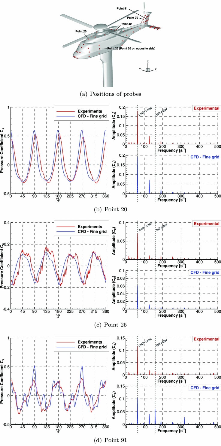
Figure 10. Pressure as function of blade azimuth (with mean value removed) and FFT decomposition of the signal for three different points on the fuselage.
5.0 DEMONSTRATION OF THE COUPLED CFD/FM METHOD
The strongly coupled HFM/HMB method described in Section III is demonstrated here for the simulation of manoeuvring rotorcraft. Coupled simulations are carried out by substituting the simplified models used for the blades, fuselage aerodynamics and inflow, with the loads predicted by CFD. Initially, the effect of the ship wake was not included in the simulations but was added later once some confidence on the tool at hand was established. The CFD loads, and the aircraft position and attitude predicted using the flight mechanics solver are exchanged at every time step of the simulation. The non-dimensional time step of
 $dt = \frac{2 \pi R}{N_{steps/cycle}} = 0.1636$
was chosen, with N
steps/cycle
= 360 and R = 9.3759. These values give 1° and 5° azimuthal steps of the main and tail rotor respectively, which is enough to ensure the stability of the CFD solver. The helicopter is trimmed before every attempt to simulate a manoeuvre and the linearised aircraft model required by the employed pilot model is computed around the trim state. The matrices used by the trimmer and the auto-pilot model are computationally expensive to generate using CFD if finite differences are used. Instead, the HFM method and simplified aerodynamics models are used, and the Jacobian matrices are computed using finite differences.
$dt = \frac{2 \pi R}{N_{steps/cycle}} = 0.1636$
was chosen, with N
steps/cycle
= 360 and R = 9.3759. These values give 1° and 5° azimuthal steps of the main and tail rotor respectively, which is enough to ensure the stability of the CFD solver. The helicopter is trimmed before every attempt to simulate a manoeuvre and the linearised aircraft model required by the employed pilot model is computed around the trim state. The matrices used by the trimmer and the auto-pilot model are computationally expensive to generate using CFD if finite differences are used. Instead, the HFM method and simplified aerodynamics models are used, and the Jacobian matrices are computed using finite differences.
5.1 Presentation of the simulations
A model of the Sea King MK50 helicopter was created for HFM from the data made available by the Aeronautical Research Laboratory of the Australian Defence Science and Technology Organisation (DSTO)(Reference Arney and Gilbert60-Reference Feik and Perrin62). Key parameters are presented in Table 3.
The helicopter is trimmed before each calculation. If the LQR auto-pilot is used, then the required matrices are calculated around the trim state, using HFM, before the manoeuvre, and are not recalculated. For CFD calculations, a trim state that best minimises the residual loads on the aircraft was used and the residual loads were removed before starting the manoeuvre.
The case of a shipborne landing manoeuvre was chosen to demonstrate the coupled HFM/HMB method. An idealised landing trajectory is shown in Fig. 11 and consists of three branches:
-
• A-B: Approach and deceleration to come to station keeping at the nominal speed of the ship.
-
• B-C: 15–20 m lateral reposition over the landing point.
-
• C-D: 10–15 m slow descent and touchdown.

Figure 11. Typical landing manoeuvre as performed by the UK Royal Navy.
The approach A-B is performed on the port side of the ship to give the pilot good visibility of the deck and ship superstructure. The lateral reposition B-C and descent C-D are performed at the nominal speed of the ship to maintain a stationary position relatively to the deck. The last two branches are critical as the helicopter must enter the ship wake and descend while maintaining an appropriate position and attitude to touchdown without over-stressing the aircraft or compromising the crew safety. The reported maximum speed for the Halifax-Class Frigate like the CPF is 29 Kn and a nominal speed of 10 m/s, or 19.4 Kn, was chosen. This speed accounts for the combination of wind and ship motion but no variation due to the atmospheric boundary-layer profile was taken into account.
A headwind case was considered. First, the B-C and C-D segments of the idealised landing trajectory were simulated using the stand-alone HFM code, with the pilot controls predicted using the embedded LQR auto-pilot model of Section 3.2. Then, the coupled HFM/HMB method is demonstrated by simulating a short ‘single-input’ response and comparing the results obtained with the trajectory predicted using the HFM method. Simulations of the shipborne helicopter in station-keeping flight at the first and last positions of the manoeuvre were then performed and the flowfields are compared. This was carried out to ensure that the Chimera method(Reference Jarkowski, Woodgate, Barakos and Rokicki73) used to interface the helicopter and ship grids was performing well, and to develop the flowfield of the ship wake. No flight mechanics model was used for these computations.
The descent manoeuvre was then performed with or without the presence of the CPF. The results were compared to identify the differences in pilot input and the aerodynamic loads due to the presence of the ship wake. In both cases, the LQR pilot model was used to track with the best accuracy possible the target trajectory.
5.2 Simulation of landing using LQR
Figures 12 and 13 show the results of a LQR-piloted simulation of the B-C and C-D branches of the manoeuvre respectively. The vehicle frame or reference is used for the results. The stand-alone HFM code was used to trim the aircraft, calculate the linearised model required for the LQR pilot model and perform the manoeuvre.

Figure 12. Aircraft position, attitude, controls history and global forces during a LQR piloted lateral reposition simulation with HFM, compared with the target trajectory. The error in x-position is shown in (a). All angles in degrees.

Figure 13. Aircraft position, attitude, controls history and global forces during a LQR piloted landing simulation with HFM, compared with the target trajectory. The error in x-position is shown in (a). All angles in degrees.
The Aeronautical Design Standard 33 ‘Handling Qualities Requirements for Military Rotorcraft’ (ADS-33E-PRF) document(Reference Standard74) specifies a series of manoeuvres that rotorcraft need to be able to perform and the associated tolerances. Results show that the LQR pilot model maintains stable flight and follows the target trajectories within the tolerance set for similar manoeuvres in the ADS33 document: the lateral reposition and the descent manoeuvres. The tolerances are represented by the shaded area in the figures.
Results for the lateral reposition manoeuvre show some overshoot in the lateral position. To alleviate this problem, some pilot models add a predictive method to ‘look-ahead’ and anticipate changes in trajectory, as in the Generalised Predictive Control (GPC) method of Hess and Jung(Reference Hess and Jung75). This limits overshoots and gives a behavioural representation of a human pilot, but it is not implemented in the current LQR model.
Moreover, accelerations of the aircraft are typically oscillatory due to the blade rotation. The position, velocities, and accelerations are time-averaged over one blade-passing period (one fifth of main rotor revolution). This is done to avoid an oscillatory response of the pilot model but introduces delays in the response.
The target trajectory given to the LQR method only specifies the change in y-position. Other targets in position and attitude angle are kept to their original value. By minimising the overall error in positioning, the LQR method allows for some deviation in every direction. To achieve the repositioning target, the helicopter needs to roll to the right to engage the translation, and to the left to exit the manoeuvre. The two peaks in attitude angle are clearly visible in Fig. 12(b) with a deviation of about 12° on each side. Forces at the rotor hub (shown as offsets of the trim value) clearly show the change in lateral force as well as a high-frequency ‘blade-passing’ signal. The pilot input in the tail rotor collective shows significant variation as a result of the changes in inflow due to the lateral velocity. There are also smaller pilot inputs on the main rotor lateral cyclic and collective to engage and exit the manoeuvre.
The target trajectory for the descent manoeuvre begins after one second of flight and covers a distance of 10 m in 4 s, while the forward velocity is kept fixed, at 10 m/s. However, the constraint was that the manoeuvre should be completed in under eight seconds. Results show that the aircraft crosses the 10 meters line six seconds after the beginning of the manoeuvre, reaches 4 m/s peak descent velocity, and then slows down to about 0.4 m/s at the 7 s mark.
The collective inputs were reduced by 2° to engage the manoeuvre before returning to the initial value. An increase in normal force can be seen at the four-second mark, which is a consequence of the reduced downwash through the rotor disk during the descent. As a consequence, no increase in rotor collective was necessary to slow down the descent and stabilise the aircraft.
5.3 Free-response to single pilot input
The coupled HFM/HMB method was first demonstrated by calculating the response of the aircraft to a single-channel pilot input. The command is a simple 2 s sinusoidal pull-up action that increases the value of the collective by 5° and then returns it to the original value as shown in Fig. 14. Other control angles were kept fixed to the initial trimmed condition.

Figure 14. Control input used to characterise the aircraft response to a single-channel pilot input.
The trimming methods only finds a trim state of the aircraft that minimises the average loading. Since the HFM helicopter model is unsteady, it does not maintain steady flight conditions even under those trimmed conditions, and ‘drifts’ if no active control is applied. This response was calculated using HFM and HMB and the resulting trajectory and attitude are shown in Fig. 15. To characterise the intrinsic response of the aircraft to the pilot input, results are presented with and without the ‘drift.’ The results obtained using the stand-alone code HFM and coupled CFD simulation are shown in Figs 16 and 17, respectively.

Figure 15. Aircraft free-response calculated with HFM and HMB if a constant pilot input is applied. This is referred to as ‘drift.’

Figure 16. Aircraft response to a collective input (Fig. 14) with and without the ‘drift.’ Position, velocities and attitude calculated using the stand-alone HFM method.

Figure 17. Aircraft response to a collective input (Fig. 14) with and without the ‘drift.’ Position, velocities and attitude calculated using the coupled HFM/HMB method.
The HFM results show a clear increase in vertical velocity and a final altitude gain of about 12 m after 6 s. The aircraft rolls and pitches as a consequence of the change in rotor loading.
The results obtained using the coupled method show a similar behaviour, albeit of lower amplitude. The total gain in altitude is about 7 m after 6 s and the rolling and pitching moments are significantly lower than predicted by the HFM simulation.
5.4 Coupled HFM/HMB simulation in free air
Figure 18 presents the test case of the final descent and landing of Fig. 13 using the coupled HFM/HMB method. The LQR pilot model is set to start after three revolutions to allow some time for the flowfield to converge. Any residual load is then removed to start the manoeuvre in trimmed flight, as can be seen in Fig. 18(d), at the 1 s mark.

Figure 18. Aircraft position, attitude, controls history and global forces during coupled CFD simulation with LQR control, compared with target trajectory. Error in x-position is shown in (a). All angles in degrees.
The results suggest that the LQR pilot accurately follows the specified trajectory with minimal deviation in terms of helicopter attitude and lateral and longitudinal positions. The LQR inputs in the main rotor cyclic and collective angles remain lower than 5°, suggesting a mild pilot activity throughout the manoeuvre. It should be noted that by construction the LQR method acts as a filter that limits high-frequency changes in control and provides optimal tracking. It is therefore not representative of the behaviour of a human pilot.
The large excursion in tail rotor collective is caused by a change in moment around the yaw axis at the beginning of the manoeuvre, probably due to a still-converging inflow on the tail rotor and an overestimated tail rotor thrust. The pilot model corrects for the deviation, without affecting the global behaviour of the aircraft.
5.5 Coupled shipborne simulations
5.5.1 Station-keeping flight
Because of the two vastly different timescales between ship and helicopter wakes, it is necessary to initialise the simulation with a larger time-step to eliminate the transient flow in the wake of the ship. Then, a set of steps are needed:
-
• The helicopter and ship speeds were set to 10 m/s. A non-dimensional time-step dt = 2.0 was used, and the rotors were kept fixed.
-
• The time step was reduced to dt = 0.1636 (corresponding to 1° steps in azimuth for the main rotor and approximately 5° for the tail rotor) and the rotors were set to rotate at their nominal speed.
-
• The residual loads were removed to avoid immediate drift from the prescribed trajectory.
-
• The simulation started with dt = 0.1636 and HFM was used to calculate the aircraft motion.
Results in Figs. 19(a) and 19(c) show the flowfield around the helicopter in isolated and shipborne conditions at the beginning of the manoeuvre. The Linear Integral Convolution method initially proposed by Cabral and Leedom(Reference Cabral and Leedom76) was used to visualise the flowfield in the moving frame of reference while the contours show the distribution of streamwise velocity. The topology of the flow around the helicopter is similar and there is a separation between the ship and helicopter wakes, with the helicopter wake being distorted by the ship wake behind the hangar. This suggests a weak effect of the ship wake on the helicopter loading at the beginning of the manoeuvre. Contours of pressure coefficient are shown and they are based on the main rotor tip velocity.
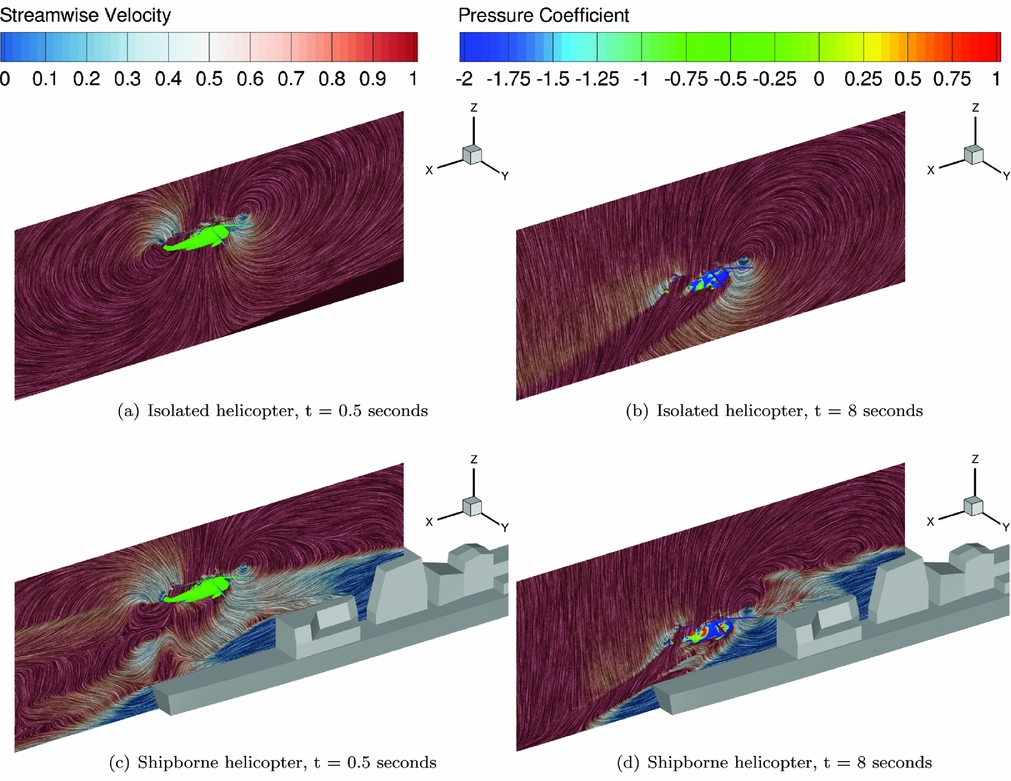
Figure 19. Flowfield visualised with LIC and pressure on the helicopter at the beginning and the end of the manoeuvre, with and without ship wake. Pressure coefficient was based on free-stream velocity.
5.5.2 Comparison between isolated and coupled responses
Results for the landing manoeuvre performed with and without the effect of the ship wake were then compared. Figure 20 shows the two pilot responses and the subsequent trajectories. As predicted, results show little influence of the ship wake at the beginning of the manoeuvre, when the helicopter is located about 15 m above the ship deck. The trajectory and pilot controls are similar until the fourth second (3 s through the manoeuvre). After 4 s, the helicopter rolling angle and lateral position show discrepancies between the two cases.

Figure 20. Comparison of the pilot and aircraft response during the piloted landing manoeuvre with (thick lines) and without (thin lines) the effect of the ship wake. All angles in degrees.
Overall, the trajectory is followed accurately and the pilot activity is similar in both instances. The rolling angle is larger in the shipborne case and the longitudinal cyclic deviates further, suggesting an increased activity of the pilot. The main rotor collective is comparatively smaller in the shipborne case despite the presence of a downwash behind the hangar. However, this can be partially explained as the main rotor plane is closer to the optimal horizontal (Φ closer to zero and Θ closer to the shaft angle of 7°) and therefore provides more vertical lift. No calculation could be performed with the helicopter at touchdown altitude because of restrictions imposed by the Chimera method. Results in terms of forces and moments are shown in Fig. 21. Despite some differences in pitching moments, the obtained loads appear very similar throughout the manoeuvre.

Figure 21. Comparison of the global forces and moments on the aircraft during the piloted landing manoeuvre with and without the effect of the ship wake.
Several surges are visible in the loads of Fig. 21, that appear when restarting the CFD computation. Future work will be carried out to ensure any restart is seamless.
Individual blade loads are shown in Fig. 22. The pitch angle of the first blade is shown with and without the harmonic content for both cases and the corresponding flapping and lead-lag aerodynamic moments at the hub are plotted. Results show similar values of loading at the beginning of the manoeuvre and discrepancies appear as the helicopter approaches the deck.

Figure 22. Comparison of the blade flapping and lead-lag moments during the piloted landing manoeuvre with and without the effect of the ship wake.
The Figs. 19(b) and 19(d) correspond to the 8 seconds time mark, with the helicopter close to the deck, and show more clearly an interaction between the two wakes. The development of the rotor wake is confined by the presence of the hangar door and deck, and extends downstream. Vortical structures that emanate from the ship superstructure are clearly visible, although they show signs of dissipation and do not seem to greatly affect the helicopter aerodynamics.
Figure 23 shows the distribution of non-dimensional w-velocity through the rotor disk at four instances during the manoeuvre. After two revolutions, the aircraft has just started descending and the isolated and shipborne cases show similar wake topologies. As the aircraft descends, it enters the ship wake and the topology of the global wake shows the presence of vortical structures that characterise the unsteadiness of the flow. The inflow velocity through the rotor disk is more important at 6 and 8 s in the shipborne case due to the downwash behind the hangar.

Figure 23. Distribution of inflow through the rotor plane during the (left) isolated manoeuvre and (right) shipborne manoeuvre.
Contours of non-dimensional w-velocity are shown in Fig. 24 on the ship symmetry plane. Traces of the vortices created in the vicinity of the ship are clearly visible, as well as the fuselage wake below the helicopter. At the 4 s mark, natural downwash combined with the rotor effect lead to an increased value of w-velocity through the rotor disk At 6 and 8 s, the apparent downwash reduces suggesting a partial ground effect caused by the deck. After 8 s, the upwash velocity of the flow between the nose of the aircraft and the hangar increases as the rotor wake is confined between the helicopter and the deck.

Figure 24. Distribution of inflow in the symmetry plane during the (left) isolated manoeuvre and (right) shipborne manoeuvre.
Figure 25 shows the distribution of the pressure coefficient on the fuselage and ship deck, five seconds into the manoeuvre. The pressure coefficient is calculated based on the freestream velocity
 $C_P = \frac{P}{\frac{1}{2} \rho U_\infty ^2}$
. The levels of C
P
show clearly the area where the helicopter wake impinges the deck. The downwash velocity is significantly higher than the freestream, leading to levels of pressure coefficient above one. The downwash over the fuselage constantly changes due to the blades passing in close proximity. Changes in pressure distribution on the fuselage are clearly visible, with high pressure levels on the boom and the roof of the cabin, and low values on the side of the aircraft where the flow accelerates.
$C_P = \frac{P}{\frac{1}{2} \rho U_\infty ^2}$
. The levels of C
P
show clearly the area where the helicopter wake impinges the deck. The downwash velocity is significantly higher than the freestream, leading to levels of pressure coefficient above one. The downwash over the fuselage constantly changes due to the blades passing in close proximity. Changes in pressure distribution on the fuselage are clearly visible, with high pressure levels on the boom and the roof of the cabin, and low values on the side of the aircraft where the flow accelerates.
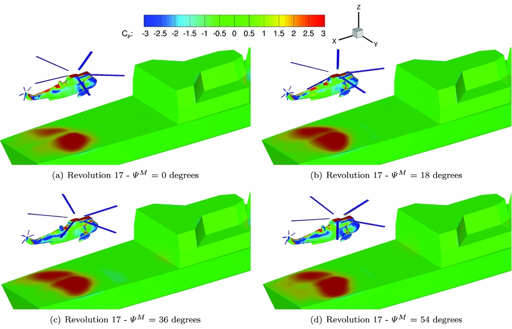
Figure 25. Distribution of pressure coefficient on the fuselage and deck at 4 azimuthal angle of the main rotor. C P scaled with the freestream velocity.
5.6 Conclusions on coupled simulations
The discrepancies between the results in the calculations of Section 5.3 suggests that the Sea King model in HFM that uses approximate aerodynamic models, poorly represents the characteristics of the aircraft obtained using the CFD. Nevertheless, despite its simplicity of the HFM model, it provided matrices for the linear models that proved accurate enough to provide good tracking performance even when using CFD.
A 10 m/s headwind case was chosen to ensure that the newly implemented method would not fail to maintain the helicopter position and attitude within a reasonable margin. More challenging flow conditions may require a more accurate linearised model, perhaps directly based on the CFD results.
The time-resolution requirement for rotor blades simulation is about one order of magnitude smaller than for ship wake simulations. It is necessary to choose the smaller time-step to ensure convergence of the solver and 1° azimuthal steps of the main rotor were chosen to limit the computational time. As a consequence, the time-accuracy for the ship wake was largely exceeding the requirements
 $\delta t < \frac{\delta x}{U_\infty }$
for the grid density used δx. The region of the deck was meshed with a typical cell size of 0.3 m, giving 50 cells per ship beam. Five newton steps were used per time step to reduce the CPU time required.
$\delta t < \frac{\delta x}{U_\infty }$
for the grid density used δx. The region of the deck was meshed with a typical cell size of 0.3 m, giving 50 cells per ship beam. Five newton steps were used per time step to reduce the CPU time required.
The k − ω SAS turbulence model used for coupled calculation proved to maintain a more reasonable level of unsteadiness than the baseline k − ω model and is more stable than the DES model. However, it only preserved the largest structures over long distances and therefore the ship wake had a lesser impact on the helicopter aerodynamics. A finer helicopter mesh would also be desirable.
6.0 SUMMARY AND CONCLUSIONS
Previous works on the simulation of ship/helicopter dynamic interface have been presented in the introduction and show that various levels of accuracy are achieved depending on the methods used and simplifications made. A full-CFD approach for manoeuvring aircraft in ship environment has not yet been considered and this paper represents a first step towards this goal, since blade aeroelasticity is not considered and the employed CFD grids are relatively coarse.
Experimental data generated for the Simple Frigate Shape 2 and the GOAHEAD full helicopter configuration was used to validate the block-structured parallel CFD solver HMB. Results show that the steady characteristics of the ship wake are well predicted and, given a good quality grid, DES and k − ω-SAS turbulence models were adequate to maintain the unsteadiness of the flowfield. The SAS model was chosen to carry out the coupled simulations due to the lower grid requirements and its numerical stability. The Test Case 2 of the GOAHEAD campaign was used to validate the performance predictions of HMB for helicopters at low advance ratio. Steady and unsteady levels of loading on the fuselage were well predicted, as well as the rotor loading despite the use of an approximate trim state predicted using the HOST tool of ONERA. These results give confidence in the ability of the HMB solver to simulate ship and helicopter wakes, and their interaction with a good accuracy.
Ship/helicopter coupled simulations were conducted using the Canadian Patrol Frigate (CPF) geometry as it is a good compromise between geometrical realism and grid complexity. The URANS k − ω SAS model was chosen after demonstrating that the URANS and DES models exhibit similar mean flow characteristics and SAS coupled reproduce similar level of unsteadiness as the DES on coarser grids and with a better numerical stability.
The Helicopter Flight Mechanics (HFM) solver was then tested as a stand-alone code and in coupled mode when implemented into the HMB environment. HFM builds a model of a helicopter based on first principles of rotorcraft flight and simple aerodynamics models. A linearisation method that computes Jacobian matrices via a second-order finite difference method was implemented and used to build a trimming method and a LQR pilot model. The helicopter was trimmed before each calculation and the linear pilot model was generated around the trimmed position. By providing a target trajectory to HFM, it is possible to simulate piloted manoeuvres, whether in stand-alone mode using simplified aerodynamics models, or in coupled mode using the CFD loads directly. Simulations of the last branch of the shipborne landing manoeuvre were performed using CFD, with and without the presence of the ship. Pilot activity and helicopter attitude show some differences, suggesting an influence of the ship wake on the aircraft.
The feasibility of simulating rotorcraft flight directly into the CFD environment was demonstrated using realistic ship and aircraft geometries, for the challenging landing manoeuvre. The trajectory was tracked with a good accuracy, despite the pilot model relying on an approximate linear model of the aircraft. Coupled simulations of the landing showed interesting results, although the dissipation of the flow solver seems to be a limiting factor. Considering that, given good quality meshes, the solver gave good predictions for both ship and helicopter wakes. It is believed that more realistic simulations of the ship/helicopter interaction can be performed by increasing the spatial and temporal discretisation, as well as increasing the convergence of the flow solver.
ACKNOWLEDGEMENTS
During this project, C. Crozon was supported by a studentship provided by AgustaWestland Ltd. The authors thank the North Eight High Performance Computing (N8 HPC) Centre for the use of the POLARIS system, as well as the ARCHIE WeST system for providing additional CPU time for computations.


