NOMENCLATURE
- ABC
-
Artificial Bee Colony
- DE
-
Differential EvolutionAlgorithm
- GA
-
Genetic Algorithm
- LQG
-
Linear Quadratic Gaussian Control
- LQI
-
Linear Quadratic Integral Control
- LQR
-
Linear Quadratic Regulator Control
- LTR
-
Loop Transfer Recovery
- MIMO
-
Multi-Input Multi-Output
- NED
-
North-East-Down Coordinates
- PEM
-
Prediction Error Minimisation Technique
- PID
-
Proportional Integral Derivative Control
- PSO
-
Particle Swarm Optimisation Algorithm
- TFL
-
Target Feedback Loop
- UAVs
-
Unmanned Aerial Vehicles
1.0 INTRODUCTION
In recent years, Unmanned Aerial Vehicles (UAVs) have gained worldwide popularity in academia and industry because of their distinguishing advantages, such as low cost, easy maintenance and good maneuverability(Reference Michael, Mellinger, Lindsey and Kumar1,Reference Maza, Kondak, Bernard and Ollero2) . As an ideal experiment platform, the great potential of UAVs has been explored for various research purposes and civil applications with different payloads, e.g. sensors, cameras or other equipment installed on the platform. Among various UAVs, the small-scale unmanned helicopters possess some unique flight capabilities such as taking off and landing vertically, flight from hovering to cruising, and flight at low altitudes. Due to their highly agile manoeuverability, small-scale helicopters have been extensively exploited in a wide variety of applications, e.g. aerial photography, electric power lines inspection, rescue services and border patrol. Therefore, research and development of the helicopters is greatly noted in academic circles(Reference Raptis, Valavanis and Vachtsevanos3,Reference Tang, Lu and Zheng4) . However, helicopters are a kind of multi-variable, strong coupling and unstable system which are more difficult to control than their fixed-wing counterparts. Designing an automatic or semi-autonomous flight controller is an essential way to expand the potential applications of the helicopters.
There are various control methods successfully implemented for helicopter in the literature. For a miniature unmanned rotorcraft, Cai et al(Reference Cai, Wang, Chen and Lee5) designed a flight control system using a Robust and Perfect Tracking (RPT) control technique. A Multi-Input Multi-Output (MIMO) trajectory controller of the helicopter using the Kalman filter-based LQI approach is reported(Reference Shin, Nonami, Fujiwara and Hazawa6). And the vision-based guidance control of a small-scale helicopter is examined by Mori et al(Reference Mori, Hirata, Tamaki and Yonezawa7). In this paper, we put forward the Linear Quadratic Gaussian/Loop Transfer Recovery (LQG/LTR) method to design an accurate tracking controller for our helicopters. This method is a systematic design approach for the multivariable system on the basis of the LQG controller and recovering open-loop singular values proposed by Doyle and Stein(Reference Stein and Athans8), which show some useful properties of robustness and some performance for the flight control system(Reference Wise9,Reference Zarei, Montazeri, Motlagh and Poshtan10) .
In the LQG/LTR or LQG design, the selection of the weighting matrices has significant impact on performance and robustness of the controller. In general, the primitive method is to set manually by the trial-and-error method. However, such a manual method is not definite and cannot find the optimal weighting matrices that meet the design specifications. Thus, some of the Evolutionary Algorithms (EAs) for selecting the weighting matrices are proposed in the literature, such as the Genetic Algorithm (GA)(Reference Barrera-Cardenas and Molinas11) is used to search the best values for the weighting matrices of LQG design, and a longitudinal LQG/LTR flight controller optimally designed based on the Differential Evolution (DE) algorithm(Reference Zhang, Sun, Cao and Zhu12). Mei and Goodal(Reference Mei and Goodall13) apply the LQG method to design a control strategy for active steering of solid axle railway vehicles and implemented the GA algorithm to search for the optimal weighting matrices of LQG. Neto et al(Reference Da Fonseca Neto, Abreu and Da Silva14) combined two computation intelligence paradigms to solve the synthesis of the Linear Quadratic Regulator (LQR) control design problem, applied GA algorithm to conduct the search of the weighting matrices and utilised the recurrent artificial neural network to solve the Riccati equation. The Artificial Bee Colony (ABC) algorithm is a novel optimisation method which imitates the swarm intelligence. The ABC algorithm was first proposed by Karaboga(Reference Karaboga and Basturk15) and has been proved to possess some advantages compared to the GA, DE and Particle Swarm Optimisation algorithm (PSO) in the function optimisation problem(Reference Karaboga and Basturk16). The principal advantage of ABC algorithm is that it can efficiently avoid local optimum to a great degree since local and global search conducted simultaneously in each iteration. The application of the ABC algorithm including optimal turning of the Proportional Integral Derivative (PID) controller(Reference Abachizadeh, Yazdi and Yousefi-Koma17), optimised LQR controller(Reference Changhao and Duan18) and Robust fuzzy Power System Stabilizer (PSS) design(Reference Abedinia, Wyns and Ghasemi19), to name a few. To the best of the authors’ knowledge, there is no report about the combination of ABC and LQG/LTR that deals with the helicopter controller design.
The outline of this paper is organised as follows. Section 2 describes the system modeling and identification of our helicopter including the experimental facilities and flight data pre-process. The basic principle of the LQG/LTR method and ABC algorithm are briefly introduced in Section 3, and a complete flight control system for trajectory tracking is well-designed based on them. The simulation result and actual flight test are presented in Section 4. Finally, the main conclusions of this paper are remarked in Section 5.
2.0 SYSTEM MODELLING AND IDENTIFICATION
In this paper, Mettler’s linearised helicopter model(Reference Mettler20,Reference Mettler, Tischler, Kanade and Messner21) is adopted to describe the dynamics of the TREX-600 small-scale unmanned helicopter. The accurate model parameters are obtained by the time-domain system identification method based on our helicopter’s flight data. This helicopter model consists of 6-Degrees-of-Freedom (DOF) rigid body dynamics and extra servo/rotor dynamics. As illustrated in Fig. 1, the dynamic motion of the helicopter is defined by the state vector x = [u v w θ ϕ q p as bs r] T in the body frame which contains the fuselage velocities (u, v, w), the angular rates (p, q, r), the main rotor flapping angles (a s , b s ) and the attitude angles (ϕ, θ, ψ).
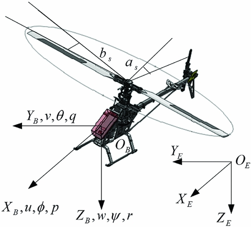
Figure 1. Illustration for helicopter states and coordinates.
The state-space model governed by Equation (1) contains a system matrix with 18 unknown parameters and a control matrix with 7 unknown parameters. This is obviously a multi-variable linear system with strong coupling. The state vectors are physically shown in the body frame, and the input vectors can be written as u = [δ col δ lat δ lon δ ped ] T , where δ col is the collective pitch and impacts heave motion (along Z B -axis); δ lat is the lateral cyclic and impacts roll motion(around X B -axis) then the lateral translation (along Y B -axis); δ lon is the longitudinal cyclic and dominates pitch motion (around Y B -axis) then the longitudinal translation (along X B -axis); δ ped is the tail rotor input and affects yaw motion (around Z B -axis) then the heading direction.
 $$\begin{equation}
\bm {\dot{x}}=\bm {Ax}+\bm {Bu},
\end{equation}$$
$$\begin{equation}
\bm {\dot{x}}=\bm {Ax}+\bm {Bu},
\end{equation}$$
where
 $$\begin{equation*}
\bm {A}=\left[ \begin{array}{c@{\;\,}c@{\;\,}c@{\;\,}c@{\;\,}c@{\;\,}c@{\;\,}c@{\;\,}c@{\;\,}c@{\;\,}c}X_u & 0 & 0 & -g & 0 & 0 & 0 & -g & 0 & 0 \\
0 & Y_u & 0 & 0 & g & 0 & 0 & 0 & g & 0 \\
0 & 0 & Z_w & 0 & 0 & 0 & 0 & Z_a & Z_b & Z_r \\
0 & 0 & 0 & 0 & 0 & 1 & 0 & 0 & 0 & 0 \\
0 & 0 & 0 & 0 & 0 & 0 & 1 & 0 & 0 & 0 \\
M_u & M_v & 0 & 0 & 0 & 1 & 0 & M_a & 0 & 0 \\
L_u & L_v & 0 & 0 & 0 & 1 & 0 & 0 & L_b & 0 \\
0 & 0 & 0 & 0 & 0 & -1 & 0 & -1/\tau & A_b & 0 \\
0 & 0 & 0 & 0 & 0 & 0 & -1 & B_a & -1/\tau & 0 \\
0 & N_v & 0 & 0 & 0 & 0 & N_p & 0 & 0 & N_r \end{array} \right], \bm {B}=\left[ \begin{array}{c@{\;\,}c@{\;\,}c@{\;\,}c}0&0&0&0\\
0&0&0&0\\
Z_{col} & 0 & 0 & 0\\
0 & 0 & 0 & 0\\
0 & 0 & 0 & 0\\
0 & 0 & 0 & 0\\
0 & 0 & 0 & 0\\
0 & A_{lat} &A_{lon}& 0\\
0 & B_{lat} &B_{lon} & 0 \\
N_{col}& 0 & 0& N_{ped} \end{array} \right]
\end{equation*}$$
$$\begin{equation*}
\bm {A}=\left[ \begin{array}{c@{\;\,}c@{\;\,}c@{\;\,}c@{\;\,}c@{\;\,}c@{\;\,}c@{\;\,}c@{\;\,}c@{\;\,}c}X_u & 0 & 0 & -g & 0 & 0 & 0 & -g & 0 & 0 \\
0 & Y_u & 0 & 0 & g & 0 & 0 & 0 & g & 0 \\
0 & 0 & Z_w & 0 & 0 & 0 & 0 & Z_a & Z_b & Z_r \\
0 & 0 & 0 & 0 & 0 & 1 & 0 & 0 & 0 & 0 \\
0 & 0 & 0 & 0 & 0 & 0 & 1 & 0 & 0 & 0 \\
M_u & M_v & 0 & 0 & 0 & 1 & 0 & M_a & 0 & 0 \\
L_u & L_v & 0 & 0 & 0 & 1 & 0 & 0 & L_b & 0 \\
0 & 0 & 0 & 0 & 0 & -1 & 0 & -1/\tau & A_b & 0 \\
0 & 0 & 0 & 0 & 0 & 0 & -1 & B_a & -1/\tau & 0 \\
0 & N_v & 0 & 0 & 0 & 0 & N_p & 0 & 0 & N_r \end{array} \right], \bm {B}=\left[ \begin{array}{c@{\;\,}c@{\;\,}c@{\;\,}c}0&0&0&0\\
0&0&0&0\\
Z_{col} & 0 & 0 & 0\\
0 & 0 & 0 & 0\\
0 & 0 & 0 & 0\\
0 & 0 & 0 & 0\\
0 & 0 & 0 & 0\\
0 & A_{lat} &A_{lon}& 0\\
0 & B_{lat} &B_{lon} & 0 \\
N_{col}& 0 & 0& N_{ped} \end{array} \right]
\end{equation*}$$
2.1 Flight experiment and data processing
The flight experiments are conducted on a modified TREX-600 small-scale helicopter equipped with a suit of on-board avionics system, as shown in Fig. 2. Table 1 gives a brief introduction of the helicopter. In order to collect the flight data, the helicopter is manipulated by a professional pilot. The AEROcontrol system is selected as a kernel unit to deliver inertial measurement through a small Inertial Measurement Unit (IMU). It provides drift-free three-axis orientation as well as calibrated three-axis acceleration, three-axis angular rate, and three-axis earth-magnetic field data. Some key parameters of the system are listed in Table 2. In addition, a low-cost GPS module is mounted on the tail beam. The specifications of the GPS, i.e. position accuracy (1 m), update rate (18 Hz) and sensitivity (−167 dBM), can meet the accuracy requirements of the flight test.
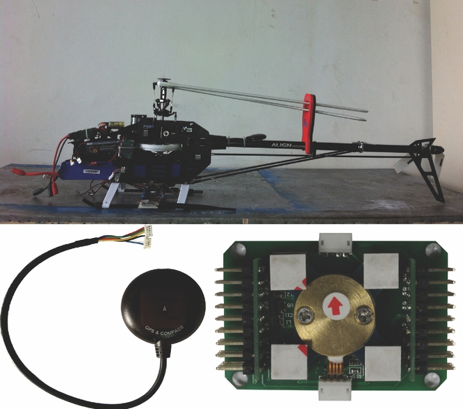
Figure 2. TREX-600 helicopter and its on-board avionics system.
Table 1 General physical parameters of TREX 600 helicopter

Table 2 Specifications of the AEROcontrol system components
In the flight tests, the pilot manually kept the helicopter in the hovering condition by regulating each channel of the control input (collective, roll, pitch and yaw). The control input and the response of the helicopter are both sampled with 50 Hz frequency and recorded in 1 GB SD card. In order to ensure that the sample size is large enough, the flight test needs to be repeated three to five times and last at least 50 s for each time.
Since the system noise and structural vibrations are unavoidable in the flight test, the pre-processing of the flight data is necessary before system identification. A five-point average finite impulse response (FIR) filter(Reference Wang and Hu22) is adopted to smooth the original data. The equation is written as:
 $$\begin{equation}
\left\lbrace \begin{array}{@{}l@{\quad }l@{}}\overline{y}_1=\frac{1}{70}[69y_1+4(y_2+y_4)-6y_3-y_5]\\[3pt]
\overline{y}_2=\frac{1}{35}[2(y_1+y_5)+27y_2+12y_3-8y_4]\\[3pt]
\overline{y}_i=\frac{1}{35}[-3(y_{i-2}+y_{i+2})+12(y_{i-1}+y_{i+1})+17y_i]\\[3pt]
\overline{y}_{m-1}=\frac{1}{35}[2(y_{m-4}+y_m)-8y_{m-3}+12y_{m-2}+27y_{m-1}]\\[3pt]
\overline{y}_{m}=\frac{1}{70}[-y_{m-4}+4(y_{m-3}+y_{m-1})-6y_{m-2}+69y_{m}] \end{array}\right. ,
\end{equation}$$
$$\begin{equation}
\left\lbrace \begin{array}{@{}l@{\quad }l@{}}\overline{y}_1=\frac{1}{70}[69y_1+4(y_2+y_4)-6y_3-y_5]\\[3pt]
\overline{y}_2=\frac{1}{35}[2(y_1+y_5)+27y_2+12y_3-8y_4]\\[3pt]
\overline{y}_i=\frac{1}{35}[-3(y_{i-2}+y_{i+2})+12(y_{i-1}+y_{i+1})+17y_i]\\[3pt]
\overline{y}_{m-1}=\frac{1}{35}[2(y_{m-4}+y_m)-8y_{m-3}+12y_{m-2}+27y_{m-1}]\\[3pt]
\overline{y}_{m}=\frac{1}{70}[-y_{m-4}+4(y_{m-3}+y_{m-1})-6y_{m-2}+69y_{m}] \end{array}\right. ,
\end{equation}$$
where Y = [y
1, . . . , y
m
]
T
is the original data, m is the data length and
 $\overline{Y}=[\overline{y}_1, .\, .\, .\, ,\overline{y}_m]^T$
is the processed data, i = 3, . . . , m − 2. The filter is based on the least square method to smooth the discrete data, in which the value of each data point is adjusted by five adjacent points using a three-order polynomial. The more that the filter is used, the smoother the curves become. However, it should be noted that overuse of the filter will lead to the increase of the identification error.
$\overline{Y}=[\overline{y}_1, .\, .\, .\, ,\overline{y}_m]^T$
is the processed data, i = 3, . . . , m − 2. The filter is based on the least square method to smooth the discrete data, in which the value of each data point is adjusted by five adjacent points using a three-order polynomial. The more that the filter is used, the smoother the curves become. However, it should be noted that overuse of the filter will lead to the increase of the identification error.
2.2 System identification and model validation
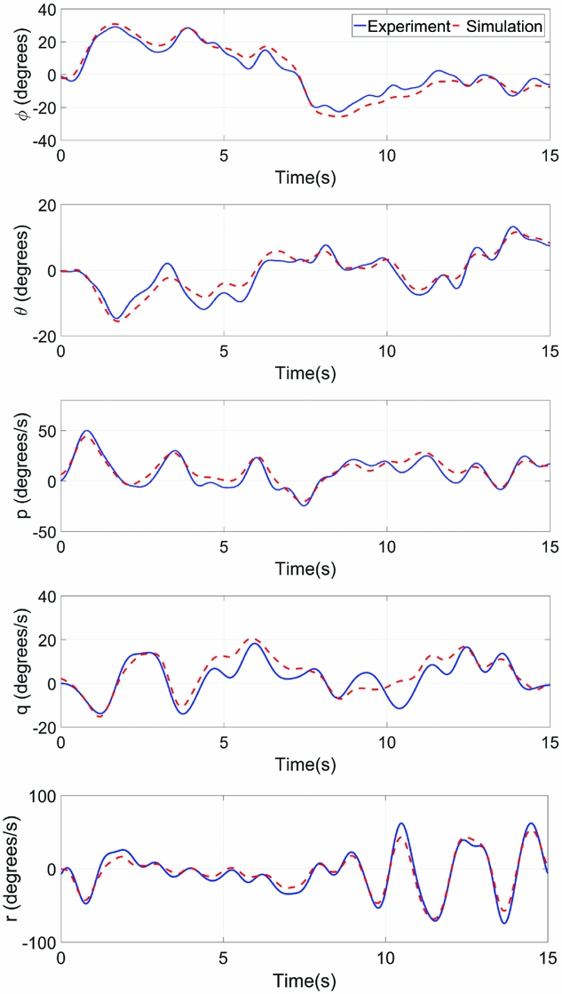
The unknown model is identified through the Prediction Error Minimisation (PEM) technique(Reference Shim, Kim and Sastry23) in the Matlab System Identification Toolbox. Here, the identification process follows Kim et al(Reference Kim, Dharmayanda, Kang, Budiyono, Lee and Adiprawita24), in which the linearised model is divided into three dynamical models: the attitude dynamics, the longitudinal and lateral velocity dynamics, and the heave velocity and yaw rate dynamics. Table 3 shows the obtained system parameters. To verify the accuracy of the identification, we compared the angular response of the obtained model with that of a manual hovering flight. Note that the angular responses of the model are gained from the simulation test using the input signals recorded in the manual flight. Figure 3 shows the identified model is able to capture the attitude dynamics of the helicopter effectively. However, with the uncertainties in the linear model, the rotor flapping dynamics is expected to have less accuracy than the attitude dynamics as the secondary system. This is mainly reflected in the distinct difference between the magnitude of A lat and B lon , which represent the effect of cyclic-on-flap for the lateral and longitudinal axes, respectively.

Figure 3. Comparison of the actual and estimated attitude responses.
Table 3 General physical parameters of TREX 600 helicopter

3.0 CONTROLLER DESIGN
In this section, a robust flight control system for our helicopter is presented based on the linear model. As depicted in Fig. 4, a two-loop hierarchical control architecture(Reference Cai, Chen and Lee25) is adopted. The inner-loop implements the LQG/LTR method to maintain the stability and decouple the helicopter dynamics. Based on the closed attitude-loop, the trajectory controller is designed by using the LQI theory to achieve good performance in local-NED-based positioning. The intermediate conversion link is responsible for the conversion of the coordinate system and control instruction.
Figure 4. Structure of the autonomous flight control system.
3.1 Attitude controller design
The attitude control of the helicopter in inner-loop is formulated as a standard LQG/LTR control problem:
 $$\begin{equation}
\left\lbrace \begin{array}{@{}l@{\quad }l@{}}\dot{\bm {x}}_{in}=\bm {A}_{in}\bm {x}_{in}+\bm {B}_{in}\bm {u}_{in}+\bm {G}w\\
\bm {y}_{in}=\bm {C}_{in}\bm {x}_{in}+\bm {v} \end{array}\!\!\!\!\!\!\right.,
\end{equation}$$
$$\begin{equation}
\left\lbrace \begin{array}{@{}l@{\quad }l@{}}\dot{\bm {x}}_{in}=\bm {A}_{in}\bm {x}_{in}+\bm {B}_{in}\bm {u}_{in}+\bm {G}w\\
\bm {y}_{in}=\bm {C}_{in}\bm {x}_{in}+\bm {v} \end{array}\!\!\!\!\!\!\right.,
\end{equation}$$
where A in , B in and C in are state space matrices of attitude dynamics which are extracted from Equation (1) by discarding the fuselage velocity vector. x in = [θ ϕ q p as bs r] T is the state vector. u in = [δ lat δ lon δ ped ] T is the control input vector and y in = [ϕ θ ψ] T is the output of the model. w and v are process disturbances and measured output noise, respectively.
In the LQG/LTR method, the first step is designing the Target Feedback Loop (TFL) which has to meet the performance and stability robustness requirements and then recovering the overall loop through the LTR procedure. In order to obtain the optimal tracking performance of the flight controller, here, the loop transfer recovery is implemented at the input of the plant. According to the separation principle, the design procedure of LQG/LTR consists of two steps:
A. TFL Design
The LQG structure with integral action is shown in Fig. 5, which increases the singular values at the low frequency band and ensures that the output y in tracks the reference command r and rejects process disturbances and measured output noise v. The optimal solution of the LQG controller, formulated in the previous section, is achieved by solving two independent optimisation problems. One is the Kalman state estimator and the other is optimal state-feedback control law. Here, the enlarged state vectors are defined as:
 $$\begin{equation}
\bm {r}=[\phi _r\ \theta _r\ \psi _r]^T, \bm {x}_i=\int _{0}^{t} (\bm {r}-\bm {y}_{in})\, dt, \overline{\bm {x}}=[\bm {x}_{in}\ \bm {x}_{i}]^T,
\end{equation}$$
$$\begin{equation}
\bm {r}=[\phi _r\ \theta _r\ \psi _r]^T, \bm {x}_i=\int _{0}^{t} (\bm {r}-\bm {y}_{in})\, dt, \overline{\bm {x}}=[\bm {x}_{in}\ \bm {x}_{i}]^T,
\end{equation}$$
where x i is the integral of the tracking error.

Figure 5. Block diagram of the LQG controller.
Then, the extended state-space system description is described by:
 $$\begin{equation}
\overline{\bm {A}}=\left[ {\begin{array}{c@{\quad}c}\bm {A}_{in}&\bm {0}\\
\bm {C}_{in}&\bm {0} \end{array}} \right], \overline{\bm {B}}=\left[ {\begin{array}{c}\bm {B}_{in}\\
\bm {0} \end{array}} \right]
\end{equation}$$
$$\begin{equation}
\overline{\bm {A}}=\left[ {\begin{array}{c@{\quad}c}\bm {A}_{in}&\bm {0}\\
\bm {C}_{in}&\bm {0} \end{array}} \right], \overline{\bm {B}}=\left[ {\begin{array}{c}\bm {B}_{in}\\
\bm {0} \end{array}} \right]
\end{equation}$$
The optimal control method is to find an optimal state-feedback control law:
 $$\begin{equation}
\bm {u}_{in}=-\bm {K}\overline{\bm {x}}=-\bm {K}_x\bm {x}_{in}-\bm {K}_i\bm {x}_{i}
\end{equation}$$
$$\begin{equation}
\bm {u}_{in}=-\bm {K}\overline{\bm {x}}=-\bm {K}_x\bm {x}_{in}-\bm {K}_i\bm {x}_{i}
\end{equation}$$
to stabilise the extended system in Equation (5) and minimise the performance index:
 $$\begin{equation}
J=\frac{1}{2}\int _{0}^{\infty } [\overline{\bm {x}}^T\bm {Q}\overline{\bm {x}}+\bm {u}_{in}^T\bm {R}\bm {u}_{in}]\, dt,
\end{equation}$$
$$\begin{equation}
J=\frac{1}{2}\int _{0}^{\infty } [\overline{\bm {x}}^T\bm {Q}\overline{\bm {x}}+\bm {u}_{in}^T\bm {R}\bm {u}_{in}]\, dt,
\end{equation}$$
where Q = diag(0, . . ., 0, n 1, n 2, n 3) ⩾ 0 and R = diag(n 4, n 4, n 4) > 0 are symmetric weight matrices, in which n i are undetermined parameters. Standard assumptions are that ( A , B ) is controllable, ( Q , A ) is observable, and R > 0.
The feedback gain is given by the solution of the algebraic Riccati equation:
 $$\begin{equation}
\left\lbrace \begin{array}{@{}l@{\quad }l@{}}\bm {K}=\bm {R}^{-1}\overline{\bm {B}}^T\bm {P}\\
\overline{\bm {A}}^T\bm {P}+\bm {P}\overline{\bm {A}}-\bm {P}\overline{\bm {B}}\bm {R}^{-1}\overline{\bm {B}}^T\bm {P}+\bm {Q}=0 \end{array}\right.
\end{equation}$$
$$\begin{equation}
\left\lbrace \begin{array}{@{}l@{\quad }l@{}}\bm {K}=\bm {R}^{-1}\overline{\bm {B}}^T\bm {P}\\
\overline{\bm {A}}^T\bm {P}+\bm {P}\overline{\bm {A}}-\bm {P}\overline{\bm {B}}\bm {R}^{-1}\overline{\bm {B}}^T\bm {P}+\bm {Q}=0 \end{array}\right.
\end{equation}$$
The TFL transfer function has the form:
 $$\begin{equation}
\bm {G}_{g}(s)=\bm {K}(s\bm {I}-\overline{\bm {A}})^{-1}\overline{\bm {B}}
\end{equation}$$
$$\begin{equation}
\bm {G}_{g}(s)=\bm {K}(s\bm {I}-\overline{\bm {A}})^{-1}\overline{\bm {B}}
\end{equation}$$
B. Kalman Filter Design and LTR Procedure
The next problem is to obtain the Kalman filter for the optimal estimate of x in , and the observer-based controller. The full-order observer is of the form:
 $$\begin{equation}
\dot{\hat{\bm {x}}}=\bm {A}_{in}\bm {\hat{x}}+\bm {B}_{in}\bm {u}_{in}+\bm {L}(\bm {y}_{in}-\bm {C}_{in}\hat{\bm {x}}),
\end{equation}$$
$$\begin{equation}
\dot{\hat{\bm {x}}}=\bm {A}_{in}\bm {\hat{x}}+\bm {B}_{in}\bm {u}_{in}+\bm {L}(\bm {y}_{in}-\bm {C}_{in}\hat{\bm {x}}),
\end{equation}$$
where
 $\hat{\bm {x}}$
is the optimal estimate of
x
in
. The Kalman filter gain
L
is given by the solution of the Riccati equation:
$\hat{\bm {x}}$
is the optimal estimate of
x
in
. The Kalman filter gain
L
is given by the solution of the Riccati equation:
 $$\begin{equation}
\left\lbrace \begin{array}{@{}l@{\quad }l@{}}\bm {L}=\bm {P}_f\bm {C}^{T}_{in}\bm {R}^{-1}_f\\
\bm {P}_f\bm {A}^{T}_{in}+\bm {A}_{in}\bm {P}_f-\bm {P}_f\bm {C}^{T}_{in}\bm {R}^{-1}_f\bm {C}_{in}\bm {P}_f+\bm {G}\bm {Q}_f\bm {G}^T=\bm {0} \end{array}\right.\!\!\!\!\!\! ,
\end{equation}$$
$$\begin{equation}
\left\lbrace \begin{array}{@{}l@{\quad }l@{}}\bm {L}=\bm {P}_f\bm {C}^{T}_{in}\bm {R}^{-1}_f\\
\bm {P}_f\bm {A}^{T}_{in}+\bm {A}_{in}\bm {P}_f-\bm {P}_f\bm {C}^{T}_{in}\bm {R}^{-1}_f\bm {C}_{in}\bm {P}_f+\bm {G}\bm {Q}_f\bm {G}^T=\bm {0} \end{array}\right.\!\!\!\!\!\! ,
\end{equation}$$
where Q f ⩾ 0 and R f ⩾ 0 are symmetric weight matrices.
The state-space realisation of the LQG controller is described by the following equations:
 \fontsize{9}{11} \selectfont{$$\begin{eqnarray}
\left[{\begin{array}{c}\dot{\hat{\bm {x}}}\\
\dot{\bm {x}}_i \end{array}}\right]= \left[{\begin{array}{c@{\quad}c}\bm {A}_{in}-\bm {B}_{in}\bm {K}_x-\bm {L}\bm {C}_{in} & -\bm {B}_{in}\bm {K}_i \\
\bm {0} & \bm {0} \end{array}} \right] \left[{\begin{array}{c}\hat{\bm {x}}\\
\bm {x}_i \end{array}} \right]+ \left[{\begin{array}{c@{\quad}c}\bm {0} & \bm {L} \\
\bm {I} & -\bm {I} \end{array}} \right] \left[{\begin{array}{c}\bm {r}\\
\bm {y} \end{array}} \right], \bm {u}=\left[{\begin{array}{c@{\quad}c}-\bm {K}_x & -\bm {K}_i \end{array}} \right] \left[{\begin{array}{c}\hat{\bm {x}} \\
\bm {x}_i \end{array}} \right] \nonumber\\
\end{eqnarray}$$}
\fontsize{9}{11} \selectfont{$$\begin{eqnarray}
\left[{\begin{array}{c}\dot{\hat{\bm {x}}}\\
\dot{\bm {x}}_i \end{array}}\right]= \left[{\begin{array}{c@{\quad}c}\bm {A}_{in}-\bm {B}_{in}\bm {K}_x-\bm {L}\bm {C}_{in} & -\bm {B}_{in}\bm {K}_i \\
\bm {0} & \bm {0} \end{array}} \right] \left[{\begin{array}{c}\hat{\bm {x}}\\
\bm {x}_i \end{array}} \right]+ \left[{\begin{array}{c@{\quad}c}\bm {0} & \bm {L} \\
\bm {I} & -\bm {I} \end{array}} \right] \left[{\begin{array}{c}\bm {r}\\
\bm {y} \end{array}} \right], \bm {u}=\left[{\begin{array}{c@{\quad}c}-\bm {K}_x & -\bm {K}_i \end{array}} \right] \left[{\begin{array}{c}\hat{\bm {x}} \\
\bm {x}_i \end{array}} \right] \nonumber\\
\end{eqnarray}$$}
The overall loop transfer function T (s) has the form:
 $$\begin{equation}
\bm {T}(s)=\bm {G}(s)\bm {G}_{LQG}(s) ,
\end{equation}$$
$$\begin{equation}
\bm {T}(s)=\bm {G}(s)\bm {G}_{LQG}(s) ,
\end{equation}$$
where G (s) = C in (s I − A in )−1 B in is the transfer function of the inner-loop plant. G LQG (s) is the transfer function of Equation (12).
The LTR procedure is conducted by assuming: Q f = ρ I , R f = I , and increasing the value ρ until the singular values of the overall loop T (s) converges to the target feedback loop G g (s) at a wide range of frequencies.
3.2 Trajectory controller design
In the field of flight control, the trajectory kinematics of an aircraft is generally characterised by:
 $$\begin{equation}
\left\lbrace \begin{array}{@{}l@{\quad }l@{}}\dot{\bm {p}}_n=\bm {v}_n\\
\dot{\bm {v}}_n=\bm {a}_n \end{array}\right.\!\!\!\!\!\!,
\end{equation}$$
$$\begin{equation}
\left\lbrace \begin{array}{@{}l@{\quad }l@{}}\dot{\bm {p}}_n=\bm {v}_n\\
\dot{\bm {v}}_n=\bm {a}_n \end{array}\right.\!\!\!\!\!\!,
\end{equation}$$
where v n = [vxvyvz ] T is the translational velocity vector, a n = [axayaz ] T is the acceleration vector, and p n = [xyz] T is the position vector. All of the vectors are described on the North-East-Down frame (NED) axes.
For the convenience of controller design, the trajectory kinematics can be rewritten in state-space model:
 $$\begin{equation}
\left\lbrace \begin{array}{@{}l@{\quad }l@{}}\dot{\bm {x}}_{out}=\bm {A}_{out}\bm {x}_{out}+\bm {B}_{out}\bm {u}_{out} \\
\bm {y}_{out}=\bm {C}_{out} \bm {x}_{out} \end{array}\right.
\end{equation}$$
$$\begin{equation}
\left\lbrace \begin{array}{@{}l@{\quad }l@{}}\dot{\bm {x}}_{out}=\bm {A}_{out}\bm {x}_{out}+\bm {B}_{out}\bm {u}_{out} \\
\bm {y}_{out}=\bm {C}_{out} \bm {x}_{out} \end{array}\right.
\end{equation}$$
 $$\begin{equation}
\bm {x}_{out}=\left[{\begin{array}{c@{\quad}c}\bm {p}_n & \bm {v}_n \end{array}}\right]^T, \bm {u}_{out}=\bm {a}_n, \bm {y}_{out}=\bm {p}_n, \bm {A}_{out}=\left[{\begin{array}{c@{\quad}c}\bm {0} & \bm {I} \\
\bm {0} & \bm {0} \end{array}}\right], \bm {B}_{out}=\left[{\begin{array}{c}\bm {0} \\
\bm {I} \end{array}}\right]
\end{equation}$$
$$\begin{equation}
\bm {x}_{out}=\left[{\begin{array}{c@{\quad}c}\bm {p}_n & \bm {v}_n \end{array}}\right]^T, \bm {u}_{out}=\bm {a}_n, \bm {y}_{out}=\bm {p}_n, \bm {A}_{out}=\left[{\begin{array}{c@{\quad}c}\bm {0} & \bm {I} \\
\bm {0} & \bm {0} \end{array}}\right], \bm {B}_{out}=\left[{\begin{array}{c}\bm {0} \\
\bm {I} \end{array}}\right]
\end{equation}$$
The point is that the position, velocity and acceleration of the helicopter are all measurable and available for feedback control. The LQI theory is employed in the design of trajectory controller as show in Fig. 6. Here, the enlarged state vectors are defined as:
Figure 6. Block diagram of the outer-loop control system.
 $$\begin{equation}
\bm {P}_{ref}=\left[{\begin{array}{c@{\quad}c@{\quad}c}x_r & y_r & z_r \end{array}}\right]^T, \bm {x}_p=\int _{0}^{t} (\bm {P}_{ref}-\bm {p}_n)\, dt, \overline{\bm {x}}_p=\left[{\begin{array}{c@{\quad}c}\bm {x}_{out} & \bm {x}_p \end{array}}\right]^T ,
\end{equation}$$
$$\begin{equation}
\bm {P}_{ref}=\left[{\begin{array}{c@{\quad}c@{\quad}c}x_r & y_r & z_r \end{array}}\right]^T, \bm {x}_p=\int _{0}^{t} (\bm {P}_{ref}-\bm {p}_n)\, dt, \overline{\bm {x}}_p=\left[{\begin{array}{c@{\quad}c}\bm {x}_{out} & \bm {x}_p \end{array}}\right]^T ,
\end{equation}$$
where P ref is the position reference and x p is the integral of tracking error.
As with Section 2.1, suppose that symmetric weight matrices of the LQI trajectory controller is Q p = diag(0, . . ., 0, n 5, n 6, n 7), R p = diag(n 8, n 8, n 8) and the optimal state-feedback control law solved from the relevant Riccati equation can be given by:
 $$\begin{equation}
\bm {u}_{out}=-\bm {F}\overline{\bm {x}}_p
\end{equation}$$
$$\begin{equation}
\bm {u}_{out}=-\bm {F}\overline{\bm {x}}_p
\end{equation}$$
3.3 Conversion unit design
As can be seen from Fig. 10, the control input
u
out
is the reference acceleration described on the NED frame, which should be converted to the command
 $\tilde{\bm {u}}=[\delta _{col} \phi _r \theta _r]^T$
. The command
$\tilde{\bm {u}}=[\delta _{col} \phi _r \theta _r]^T$
. The command
 $\tilde{\bm {u}}$
is the dominator of body-axis acceleration. The collective control input δ
col
is transferred from
u
out
since it dominates heave acceleration. And the heading direction ψ
r
is relatively independent of linear motion for helicopters, which is pre-established. Thus, the design processes of the conversion unit consist of two steps:
$\tilde{\bm {u}}$
is the dominator of body-axis acceleration. The collective control input δ
col
is transferred from
u
out
since it dominates heave acceleration. And the heading direction ψ
r
is relatively independent of linear motion for helicopters, which is pre-established. Thus, the design processes of the conversion unit consist of two steps:
Step 1. Convert from NED acceleration command u out to body-axis acceleration command u b, r and simply conduct by the dynamic inverse of the rotation matrix:
 $$\begin{equation}
\bm {u}_{b,r}=-\bm {R}^{-1}\bm {u}_{out}
\end{equation}$$
$$\begin{equation}
\bm {u}_{b,r}=-\bm {R}^{-1}\bm {u}_{out}
\end{equation}$$
Step 2. Convert the acceleration command
u
b, r
to the body-axis acceleration command
 $\tilde{\bm {u}}=[\delta _{col} \phi _r \theta _r]^T$
. After the control law in Equation (6) is calculated, the dynamics of the closed attitude-loop can be characterised by:
$\tilde{\bm {u}}=[\delta _{col} \phi _r \theta _r]^T$
. After the control law in Equation (6) is calculated, the dynamics of the closed attitude-loop can be characterised by:
 $$\begin{equation}
\dot{\overline{\bm {x}}}=\bm {A}_k\overline{\bm {x}}+\bm {B}_k\bm {r} \bm {u}_{out}=-\bm {F}_p
\end{equation}$$
$$\begin{equation}
\dot{\overline{\bm {x}}}=\bm {A}_k\overline{\bm {x}}+\bm {B}_k\bm {r} \bm {u}_{out}=-\bm {F}_p
\end{equation}$$
 $$\begin{equation}
\bm {A}_k=\left[{\begin{array}{c@{\quad}c}\bm {A}_{in}-\bm {B}_{in}\bm {K}_x & -\bm {B}_{in}\bm {K}_i\\
-\bm {C}_{in} & \bm {0} \end{array}}\right], \bm {B}_k=\left[{\begin{array}{c}\bm {0}\\
\bm {I} \end{array}}\right] ,
\end{equation}$$
$$\begin{equation}
\bm {A}_k=\left[{\begin{array}{c@{\quad}c}\bm {A}_{in}-\bm {B}_{in}\bm {K}_x & -\bm {B}_{in}\bm {K}_i\\
-\bm {C}_{in} & \bm {0} \end{array}}\right], \bm {B}_k=\left[{\begin{array}{c}\bm {0}\\
\bm {I} \end{array}}\right] ,
\end{equation}$$
and here, treated the body-axis acceleration a b as the system output, which represents the correlation of the outer loop with the inner loop:
 $$\begin{equation}
\left\lbrace \begin{array}{@{}l@{\quad }l@{}}\dot{\overline{\bm {x}}}=\bm {A}_{k}\overline{\bm {x}}+\tilde{\bm {B}}_k\tilde{\bm {u}} \\
\bm {a}_b=\bm {C}_g \overline{\bm {x}}+\bm {D}_g\tilde{\bm {u}} \end{array}\right.\!\!\!\!\!\!,
\end{equation}$$
$$\begin{equation}
\left\lbrace \begin{array}{@{}l@{\quad }l@{}}\dot{\overline{\bm {x}}}=\bm {A}_{k}\overline{\bm {x}}+\tilde{\bm {B}}_k\tilde{\bm {u}} \\
\bm {a}_b=\bm {C}_g \overline{\bm {x}}+\bm {D}_g\tilde{\bm {u}} \end{array}\right.\!\!\!\!\!\!,
\end{equation}$$
where
 $\tilde{\bm {B}}_k$
consists of the first two columns of
B
k
.
C
g
and
D
g
are extracted from helicopter model Equation (1).
$\tilde{\bm {B}}_k$
consists of the first two columns of
B
k
.
C
g
and
D
g
are extracted from helicopter model Equation (1).
Note that the system is stable, the steady-state gain matrix
G
a
from
 $\tilde{\bm {u}}$
to
a
b
is calculated by the following equation:
$\tilde{\bm {u}}$
to
a
b
is calculated by the following equation:
 $$\begin{equation}
\bm {G}_a=-\bm {C}_g\bm {A}_k^{-1}\tilde{\bm {B}}_k+\bm {D}_g
\end{equation}$$
$$\begin{equation}
\bm {G}_a=-\bm {C}_g\bm {A}_k^{-1}\tilde{\bm {B}}_k+\bm {D}_g
\end{equation}$$
The feasibility of this design idea is illustrated in(Reference Wang, Chen and Lee26), and later the flight tests show that it is available for our helicopter. In summary, the conversion unit from
u
out
to
 $\tilde{\bm {u}}$
is computed by:
$\tilde{\bm {u}}$
is computed by:
 $$\begin{equation}
\tilde{\bm {u}}=-\bm {G}_a^{-1}\bm {R}^{-1}\bm {u}_{out}
\end{equation}$$
$$\begin{equation}
\tilde{\bm {u}}=-\bm {G}_a^{-1}\bm {R}^{-1}\bm {u}_{out}
\end{equation}$$
3.4 ABC optimisation of LQG/LTR flight controller
As mentioned in Section 3, it is necessary that the undetermined parameters n i (i = 1,. . ., 8) for four weighting matrices ( Q , R , Q p , R p ) should be selected to solve the Riccati equations and get the feedback gain K and F . Based on the result, the conversion unit and optimal Kalman filter using LTR are also obtained. For this purpose, a methodology based on ABC is implemented to automatically search for the optimal weighting matrices. ABC is a simulation of honey bees swarm behaviour that consists of three essential components, i.e. unemployed bees, employed bees and food sources. To implement ABC to search the best values of the weighting matrices, the food source is defined as a possible solution vector of the undetermined parameters and its property is quantified by the fitness values. Employed bees are associated with a particular food source. Unemployed bees constantly search around the food source which contains two types of unemployed bees: scouts and onlookers. The implementation procedure of the proposed methodology can be described as follows:
Step 1. Population initialisation: Randomly initialise a set of possible solution vectors x i (i = 1, . . ., SN) which is computed by Equation (25). Here, SN is the total number of food source; the number of employed bees and unemployed bees is both equal to SN/2.
 $$\begin{equation}
\left\lbrace \begin{array}{@{}l@{\quad }l@{}}\bm {x}_i=(x_{i1}, x_{i2},\ldots ,x_{i8}) \\
x_{ij}=x_{min}+rand(0,1)\times (x_{max}-x_{min}) \end{array}\right.\!\!\!\!\!\!,
\end{equation}$$
$$\begin{equation}
\left\lbrace \begin{array}{@{}l@{\quad }l@{}}\bm {x}_i=(x_{i1}, x_{i2},\ldots ,x_{i8}) \\
x_{ij}=x_{min}+rand(0,1)\times (x_{max}-x_{min}) \end{array}\right.\!\!\!\!\!\!,
\end{equation}$$
where x ij is the elements of food source. x min and x max mean the lower and upper bounds, respectively.
Step 2. Fitness values: The compute of fitness value is based on the step response of the closed-loop system. It is a crucial step in applying ABC that selects the objective function used to evaluate the fitness of each possible solution x i . Here, the performance indices Integral of Time multiplied by Absolute Error (ITAE) is used for that purpose. The linearised system of Equation (1) is used to get the step response and calculate the fitness value. According to the following equations, fitness values for each x i are calculated and select the top SN/2 best solutions as the initial population of the employed bees.
 $$\begin{equation}
\left\lbrace \begin{array}{@{}l@{\quad }l@{}}fit_i=\frac{1}{1+F_i}\\[10pt]
F_i=\int _{0}^{\infty } [l_1te(t)+l_2\bm {u}^T\bm {u}]\, dt \end{array}\right.\!\!\!\!\!\!,
\end{equation}$$
$$\begin{equation}
\left\lbrace \begin{array}{@{}l@{\quad }l@{}}fit_i=\frac{1}{1+F_i}\\[10pt]
F_i=\int _{0}^{\infty } [l_1te(t)+l_2\bm {u}^T\bm {u}]\, dt \end{array}\right.\!\!\!\!\!\!,
\end{equation}$$
where fit i is the fitness value, F i is the objective function, e(t) is the trajectory tracking error in the time domain, and u is the input vectors of the helicopter. l i is the normalisation factor.
Step 3. Employed bee search: In the iter iteration, each employed bee searches new solutions in the neighborhood of the current solutions vector by Equation (27) and chooses the better solution between new solution v i and original solution x i of employed bees into the next generation.
 $$\begin{equation}
\left\lbrace \begin{array}{@{}l@{\quad }l@{}}\bm {v}_i=(v_{i1},\ldots ,v_{ij},\ldots ),v_{i8}\\
v_{ij}=x_{ij}^{iter}+rand(-1,1)\times (x_{ij}^{iter}-x_{kj}^{iter}),(k\ne i) \end{array}\right.\!\!\!\!\!\!,
\end{equation}$$
$$\begin{equation}
\left\lbrace \begin{array}{@{}l@{\quad }l@{}}\bm {v}_i=(v_{i1},\ldots ,v_{ij},\ldots ),v_{i8}\\
v_{ij}=x_{ij}^{iter}+rand(-1,1)\times (x_{ij}^{iter}-x_{kj}^{iter}),(k\ne i) \end{array}\right.\!\!\!\!\!\!,
\end{equation}$$
where v i is the new solution randomly generated. i and k are randomly generated; rand( −1, 1) means a random number in the range from −1 to 1.
Step 4. Unemployed bee search: Each unemployed bee chooses an employed bee to trace according to their probability values. The formula of the probability method can be described as follows:
 $$\begin{equation}
p_i=\frac{fit_i}{\sum _{i=1}^{SN/2} fit_i}
\end{equation}$$
$$\begin{equation}
p_i=\frac{fit_i}{\sum _{i=1}^{SN/2} fit_i}
\end{equation}$$
Step 5. Scouter search: If the search time trial exceeds the predetermined threshold limit, but the optimal value cannot be improved, then the food source should be deserted and its employed bee changed to scouter bees. The solution vector can be re-initialised according to Equation (27).
Step 6. Iteration: Store the best solution vectors achieved at the present time and go back to Step 3 until termination criteria I max is met.
Step 7. LTR Procedure: Since the best solution of weighting matrices were obtained by the algorithm, the LTR can be conducted at the input of the plant as mentioned in Section 3.1.
The flow chart of the ABC optimisation of the LQG/LTR method can be seen in Fig. 7.

Figure 7. The procedure of the proposed method.
4.0 FLIGHT EXPERIMENT AND SIMULATION RESULTS
4.1 Simulation result
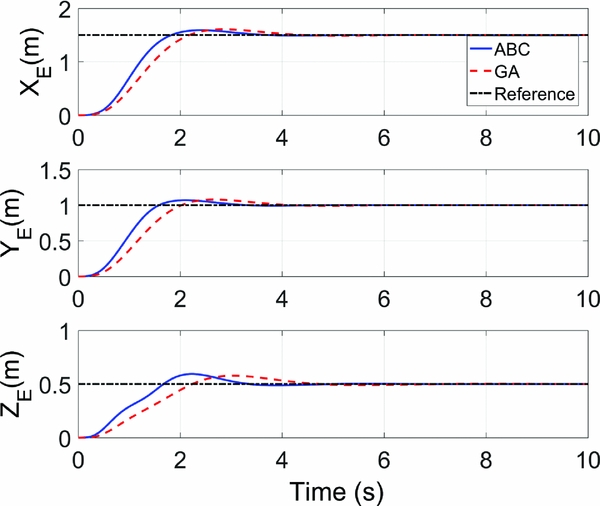
The optimization of LQG/LTR controller is carried out with the proposed method in Matlab 2012b environment. The simulation parameters of ABC, i.e. the total number of bees SN = 20, and the threshold limit = 5. In addition, a comparison of the GA algorithm(Reference Karaboga and Basturk16) with ABC is also conducted to validate the feasibility of ABC. The GA parameters, i.e. population size, crossover probability and mutation probability, are chosen as 20, 0.8 and 0.2. With the same objective function and feedback control loop, the Matlab programs are built up based onthe ABC and GA algorithms, respectively. Figure 8 records the optimal value of objective function F i calculated by ABC and GA in each iteration. As can be seen in the figure, although the ABC algorithm starts at a worse initial value due to the randomness of population initialisation, it has a lower final value and faster converge rate than the GA algorithm. As shown in Fig. 9, the responses of the different step signals demonstrate the decoupling performance of the controller. The results also indicated that the proposed method achieves better control performance in terms of overshoot percentage, rising time and settling time. The recovery process for different values of ρ is depicted in Fig. 10. Once the feedback control loop G g (s) is optimised, we adjust the observer gain L until the overall closed-loop T (s) recovers internal stability and some of the robustness properties (singular values) of the feedback loop G g (s). It illustrates that as the value of ρ increases, the three singular values are close to each other finally which means a good following performance and disturbance rejection.
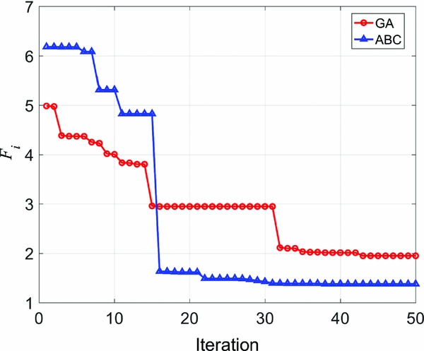
Figure 8. Evolution curves of ABC and GA.

Figure 9. Step response of closed-loop system.
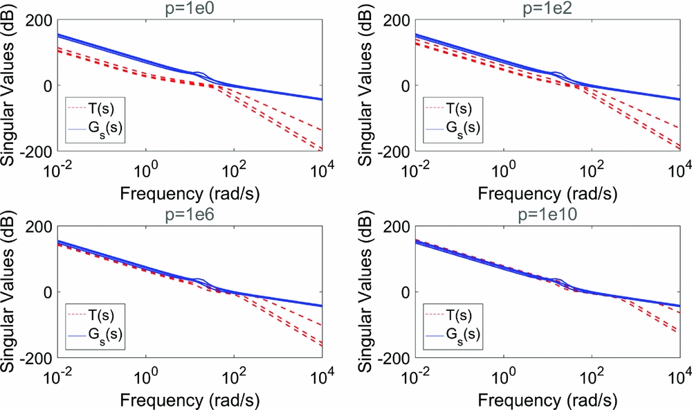
Figure 10. The loop transfer recovery process for different values of ρ.
4.2 Flight test result
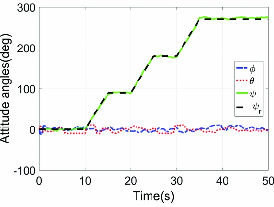
Actual flight experiments are conducted by the optimal LQG/LTR controller described in the previous section. The trajectory tracking results in one test are depicted in Figs 11–13. Figure 11 presents the 3D flight trajectory. The predefined path starts at point A, turns right while hovering at point B, D and E with yaw reference ψ r , and finally ends with hovering at point F, lasting 10 s. Figure 12 presents the yaw reference and the fuselage attitude angles measured by the IMU and shows that the yaw control is available and the fuselage are well stabilised. Figure 13 gives the fuselage velocities u, v and w in the flight test. Combining that with Fig. 12, we can distinguish the different flight sections explicitly. In brief, the form of the designed controller is as simple as a MIMO controller and all of the determinable parameters are selected automatically, which display promising application prospects.
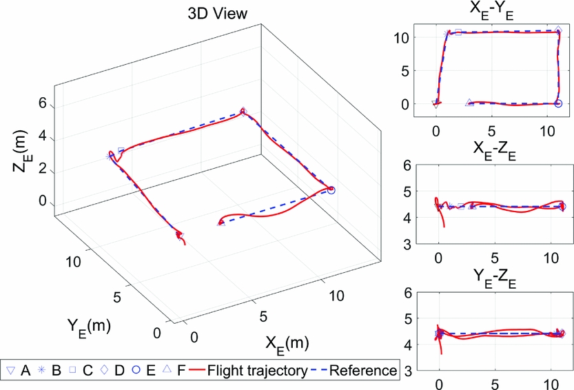
Figure 11. Actual 3D flight trajectory under the control of optimal LQG/LTR in NED frame.

Figure 12. Attitude angles in the flight test.
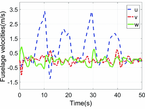
Figure 13. Fuselage velocities in the flight test.
5.0 CONCLUSION
This paper presents a novel LQG/LTR optimal design method based on the ABC algorithm applied to trajectory tracking of a small-scale helicopter. To implement this method, the linear model of the helicopter is identified from flight data and the ABC algorithm is used to automate the search for the controller parameters. The Kalman filter gain in LQG design is adjusted after the feedback loop is optimised. A series of flight experiments and simulations are conducted. Simulation results suggest that compared with GA optimisation algorithm, our proposed method achieves a better result with smaller objective function value and preferable step response of the controller. In flight tests, the optimal controller performs well in hovering, yaw control and trajectory tracking, proving that our proposed method is feasible and robust.
ACKNOWLEDGEMENTS
This work was partially supported by the National Natural Sciences Foundation of China (51375230) and the project of Science and Technology Support Plan of Jiangsu province (BE2013003-1 and BE2013010-2).