NOMENCLATURE
- A
-
slot area m 2
- C 1, C 2
-
equation constants
- C μ
-
blowing momentum coefficient %
- D
-
primary nozzle diameter m
- F
-
surface integral of the rate of change of the momentum N
-
 $f(\vec{x})$
-
objective (Cost) function
-
$g(\vec{x})$
-
constraint function
-
$\dot{m}$
-
jet Mass flux kg/s
- n
-
number of design variables
-
$\bar{q}\,$
-
dynamic pressure N/m 2
- R
-
Coanda surface radius m
- S
-
primary nozzle reference area m 2
- V
-
flow velocity m/s
-
$\vec{x}$
-
optimisation design vector
-
${\vec{x}_r}$
-
vector of reference values
- δ
-
angle function
$\deg $
- δ T
-
thrust deflection angle
$\deg $
- θ
-
coanda surface cut-off angle
$\deg $
- κ
-
secondary slot arc length over the primary slot circumference
- λ*
-
appropriate step length in optimisation
- ρ
-
flow density kg/m 3
- CFD
-
Computational Fluid Dynamics
- FTV
-
Fluidic Thrust Vectoring
- RPM
-
Revolution Per Minute
- V/STOL
-
Vertical or Short Take-Off and Landing
- p
-
Associated with the primary flow
- s
-
Associated with the secondary flow


Acronym
Subscript
1.0 INTRODUCTION
Thrust vectoring has found increasing applications in recent years. The need for simple, reliable and effective Vertical or Short Take-Off and Landing (V/STOL) aircraft, operating from small areas has opened up opportunities for utilisation and application of thrust vectoring concepts(Reference Páscoa and Dumas1). These concepts have been extensively studied in the past from both computational and experimental viewpoints(Reference Saghafl and Banazadeh2). Depending on the flight condition, the aircraft weight and the moment arm, the thrust can be successfully deflected through as much as 90° to perform required manoeuvres. Two major methods have been employed to vector the exhaust gases of an engine until the present time. The conventional methods, which rely on mechanical means, and the most recent methods, which are fluidic-based thrust vectoring techniques(Reference Kowal3,Reference Flamm4) . Fluidic thrust vectoring is based on using secondary air stream to deflect the primary jet. In contrast to the conventional mechanical thrust vectoring systems, fluidic systems require few or no moving parts. Moreover, they result in a fast dynamic response compared to those achieved by mechanical actuators. These systems also reduce weight and complexity(Reference Stryowski and Schmid5). To date, there have been a variety of approaches to Fluidic Thrust Vectoring (FTV) design, which include the use of synthetic jet actuators, counter flows, co-flows, throat skewing techniques and shock-wave manipulation(Reference Kowal3,Reference Flamm4) .
In literature, a circulation jet that entrains the engine exhaust gases to change and control thrust direction is called co-flow fluidic thrust vectoring. The so-called co-flow technique is based on the well-known Coanda effect phenomenon. Coanda effect is the natural tendency of fluid and gaseous jets to attach to a wall which is projected close to them(Reference Triboix and Marchchal6). The stream remains attached to the wall as a result of the balance of inertial centrifugal force and sub-ambient static pressure within the stream(Reference Carpenter and Green7). This causes the fluid to follow the convex curvature of the solid boundary and deviate from a straight course, as seen in Fig. 1.

Figure 1. (a) Schematic illustration of the Coanda effect, (b) CFD simulation, and (c) close-up view of the vortices and boundary layer.
Here, as a result of a rise in the viscous shear stress, the boundary layer expands and thus reduces the fluid velocity. Therefore, the fluid detaches from the surface at a new stagnation point. Separation of this fluid could be controlled or enhanced by blowing a secondary flow. The secondary flow itself is introduced via a slot, which expels it tangentially over the surface and adds momentum to the boundary layer to make the well-known Coanda effect. With the curved surface, the Kutta condition does not apply. Therefore, the flow turning and separation location are altered based on the rate of mass or momentum addition(Reference Schlichting and Gersten8). To enhance the efficiency, momentum flux of the secondary jet should be large compared to that of the primary flow. The nature of this phenomenon is extremely complex. It is known that no unique solution exists to analytically solve the flow(Reference Wille and Fernholz9). Accordingly, recent achievements in this area are totally based on extensive experimental results(Reference Banazadeh and Behroo10). Rask and Patankar have studied two- and three-dimensional curved wall jets(Reference Rask11,Reference Patankar and Sridhar12) . Similar arrangement is used on planar geometries for thrust vectoring by Mason and Crowther(Reference Mason and Crowther13).
While modern fluidic nozzles are designed and developed to increase the thrust vectoring efficiency(Reference Gu, Xu and Guo14), to the author's knowledge, limited academic research has been performed on fluidic nozzles, especially multi-directional cylindrical ones. In general, parameters that affect the flow ability to remain attached to the curved surface include the free-stream velocity, radius of curvature, slot location and size (height and span) and blowing pressure(Reference Banazadeh and Saghafi15). In the current study, a microjet engine exhaust nozzle is connected to an additional cylindrical duct with a bell mouth shape, circumferentially divided into four identical secondary flow channels for multi-directional thrust vectoring (Fig. 2). During the experiments, the upper slots are the only active slot and the secondary co-flowing stream is established along them.
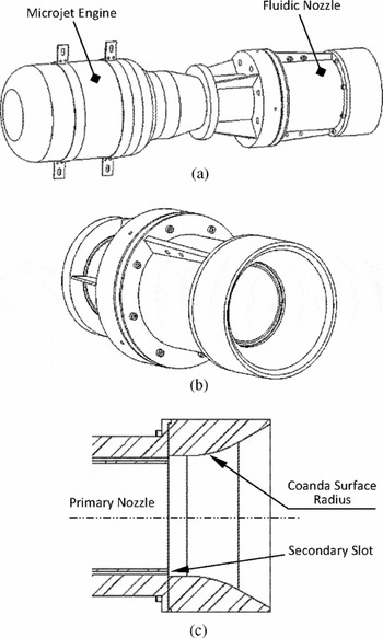
Figure 2. (a) Isometric view of the fluidic nozzle mounted on the engine, (b) isometric close-up of the fluidic nozzle, and (c) a cross-sectional view of the nozzle architecture.
As shown in Fig. 2(c), the exhaust nozzle ends to a small step, which previous studies have found it to be useful in turning the flow into eddy to form what is called a ring vortex and make the FTV system more efficient(Reference Le, Moin and Kim16). The effectiveness of the step greatly depends on the size and the flow properties, regarding the Reynolds number. This phenomenon was investigated by the authors, using numerical simulations for step sizes less than 1 mm. However, due to manufacturing and instrumentation constraints it is not possible to experimentally examine the effectiveness and details of the events happening on the corner and over the collar surface. Hence, a very small step at the size of 0.2 mm was chosen for this research to take the observation into account, when preparing an automatic grid generation file to perform sensitivity analysis and parametric study by numerical simulations. A Coanda surface with a circular shape is appended to this step.
Here, the shape of the wall and the relative blowing momentum of the fluid that is injected through the slot, control the location of the surface stagnation point and therefore the thrust deflection angle. For a constant wall shape, the deflection angle is controlled by the non-dimensional parameter C μ, defined using secondary and primary flow properties:
 $$\begin{equation}
{C_\mu } = \,\frac{{\dot{m}{V_s}}}{{\bar{q}S}}\, = \,\frac{{2{\rho _s}{A_s}V_s^2}}{{{\rho _p}V_p^2S}}\,,
\end{equation}$$
$$\begin{equation}
{C_\mu } = \,\frac{{\dot{m}{V_s}}}{{\bar{q}S}}\, = \,\frac{{2{\rho _s}{A_s}V_s^2}}{{{\rho _p}V_p^2S}}\,,
\end{equation}$$
where C
μ is widely known in the literature as blowing momentum coefficient(Reference Joslin and Jones17),
 $\dot{m}$
is the secondary jet mass flux, S is the primary nozzle reference area, VP
is the primary flow velocity and Vs
is the secondary jet velocity. Regarding a constant value for C
μ, the deflection angle could also be changed by altering the surface geometry. In this study, thrust vectoring performance is obtained for different primary and secondary air flows, while the non-dimensional geometric parameters are variable. Basic geometric parameters and flow properties of the fluidic nozzle are presented in Table 1.
$\dot{m}$
is the secondary jet mass flux, S is the primary nozzle reference area, VP
is the primary flow velocity and Vs
is the secondary jet velocity. Regarding a constant value for C
μ, the deflection angle could also be changed by altering the surface geometry. In this study, thrust vectoring performance is obtained for different primary and secondary air flows, while the non-dimensional geometric parameters are variable. Basic geometric parameters and flow properties of the fluidic nozzle are presented in Table 1.
Table 1 Geometric parameters and flow rate ratios for the fluidic nozzle

Allen tried to find the variation of vectoring angle for a non-rotating axisymmetric Coanda-assisted flow as a function of the exit geometry and flow parameters(Reference Allen18). A correlation function is introduced that enables the prediction of vectoring angle for a given momentum ratio, collar radius and exit slot circumference percentage. This function is described in Equation (2):
 $$\begin{equation}
\delta = {\left({C_1} \times {J^*} \times \frac{a}{D}\right)^{(\kappa /{C_2})}},
\end{equation}$$
$$\begin{equation}
\delta = {\left({C_1} \times {J^*} \times \frac{a}{D}\right)^{(\kappa /{C_2})}},
\end{equation}$$
where δ is the angle function with the unit of degree, J* has the same value of C
μ but defined as the momentum flux ratio,
 $\frac{a}{D}$
is the collar radius to the primary jet diameter ratio and κ is the control slot circumference over the primary slot circumference. The constants, C
1 and C
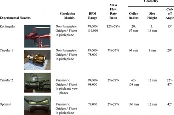
2, have empirical values of 3.25 and 2.0, as found by Allen. The intention of the present paper is mainly to investigate the dependency of the deflection angle on nozzle geometry and secondary to primary flow ratios in a co-flow fluidic thrust vectoring system. To achieve this goal, as presented in Fig. 3 and listed in Table 2, different nozzles including one rectangular and two circular sections have been built and experimentally tested to gather data for different secondary to primary mass flow ratios. To improve the validity of the results by increasing the number of data, other geometrically different nozzles have also been considered, some of which from a parallel investigation process on the nozzle geometry optimisation for the best thrust vectoring angle, and analysed computationally using a previously developed and validated CFD simulation models(Reference Banazadeh and Saghafi15,Reference Banazadeh and Saghafi19) . The validation of the models has been carried out by the use of the experimental test data of the already mentioned physically built nozzles. Accordingly, there have been two parallel research process, fully linked together, on finding correlation between thrust vectoring angle and flow/nozzle characteristics. The current paper presents a report on both related researches and results.
$\frac{a}{D}$
is the collar radius to the primary jet diameter ratio and κ is the control slot circumference over the primary slot circumference. The constants, C
1 and C
2, have empirical values of 3.25 and 2.0, as found by Allen. The intention of the present paper is mainly to investigate the dependency of the deflection angle on nozzle geometry and secondary to primary flow ratios in a co-flow fluidic thrust vectoring system. To achieve this goal, as presented in Fig. 3 and listed in Table 2, different nozzles including one rectangular and two circular sections have been built and experimentally tested to gather data for different secondary to primary mass flow ratios. To improve the validity of the results by increasing the number of data, other geometrically different nozzles have also been considered, some of which from a parallel investigation process on the nozzle geometry optimisation for the best thrust vectoring angle, and analysed computationally using a previously developed and validated CFD simulation models(Reference Banazadeh and Saghafi15,Reference Banazadeh and Saghafi19) . The validation of the models has been carried out by the use of the experimental test data of the already mentioned physically built nozzles. Accordingly, there have been two parallel research process, fully linked together, on finding correlation between thrust vectoring angle and flow/nozzle characteristics. The current paper presents a report on both related researches and results.

Figure 3. The research review flow chart.
Table 2 Summary of experimental work in the process of analysis and validation
At first, the experimental facility and measurements will be described. Then a useful empirical formulation is derived for thrust vectoring angle, based on a series of tests carried out on small jet engines. This angle is closely related to the momentum coefficient, secondary slot height, Coanda surface radius and primary nozzle diameter. Here, computational fluid dynamics simulation is utilised to predict the system behaviour. Once a validated CFD model is developed, it will be used for geometric optimisation without the need for extensive and expensive experimental set-ups. The scripting language and the ability to define and use variables in some CFD meshing software produce a scripted record of the user interactive session and also provide parametric study capability(20). This capability allows us to securely investigate the influence of one or more geometric parameters on the model performance, when designing a FTV system. Utilising a numerical optimisation process, this investigation could lead to an optimal nozzle geometry for the maximum thrust deflection angle(Reference Saghafi and Banazadeh21). In the current study, it is desired to find a Coanda surface geometry that maximises thrust-vector angle in a constant blowing momentum coefficient.
2.0 EXPERIMENTAL ARRANGEMENT
AMT Olympus engines, both the original version and the high-performance one, were used as propulsion systems to provide the primary stream for the test set-up(22). These engines have a single radial compressor, an axial turbine and annular type combustion chamber. The engines diameter and length are approximately 130 × 374 mm. For these engines, the total pressure ratio was estimated (and also reported by the manufacturer) to be around 4, and the maximum exhaust gas temperature was measured to be 750 K. For the high-performance version, maximum thrust, corresponding to the standard ambient condition, and maximum air mass flow rate were measured to be 230 N and 450 gr/s, which occurred at 110,000 rpm. The time required for the turbine to spool up from minimum to maximum speed is 4 seconds and back to the minimum is 3 seconds. The engine cooling and lubrication is done via the oil/fuel mixture. As shown in Fig. 4, the secondary flow is generated by a 80 L reservoir that is connected via a 40 psi solenoid valve to the air compressor, which provides an air mass flow rate of 12 m3/h at the maximum pressure of 325 atm.

Figure 4. (a) Air compressor and reservoir and (b) fluidic nozzles.
The axial thrust is measured by use of two bending-beam load cells, placed on the sides of the engine cradle, as shown in Fig. 5. Load cells have gone through calibration process before the test setup and biases are removed at the beginning of each test. The pitching and yawing moments are measured through torque meters that are installed on the sides and underneath of the external cradle. The entire output, including load cells, torque meters, flow meter, pressure and time data are collected using a digital data acquisition system at the frequency of 5 Hz. The final experimental arrangement is shown in Fig. 5(b). Here, the jet engine and the fluidic nozzle are mounted on the cradle and the axial force of the engine is applied to the single point load cells in order to measure the axial thrust. This cradle is supported by another external cradle, using pivots, and is able to rotate around the pitching axis. The whole system is also supported by the main stand that is able to rotate about the vertical hinge to examine the yaw force.

Figure 5. (a) Proposed experimental arrangement and (b) final experimental set-up.
By this technique, it is possible to measure the axial and side forces that can be used for the calculation of thrust deflection angle. The thrust can be deflected in two directions, depending on the active secondary air channel. Multiple tests are conducted in an outdoor space, in which the engine exhaust is vented to the atmosphere. This confirms the accuracy of the boundary condition setting of the computational model as well as the experimental measurements. Two parallel pipes are considered for every channel to provide a uniform flow distribution in the reservoir, just before the slot. These pipes are connected to the nozzle by push-in connectors and to the main pipes by two-way push-in dividers. The main pipes are suspended by a support element to freely move around as a result of the reaction force. The set-up is also optimised for free rotation at the beginning of each test, by using flexible pipes, adding wall clearance and adjusting the centre of gravity position. Pipe reaction forces are also calculated for the secondary line and excluded from the data, considering the pressure difference between the main reservoir and the nozzle accumulator to compute the air mass flow rate passing through the glass tube flowmeter, and hence to come up with the reaction force. This force and the resultant torque is double checked with the one that is measured by the torque meters. Other sources of uncertainties like pressure fluctuations and system backlash are also removed from the data by an offline data reduction procedure. It is notable again that all the sensors received a factory and user calibration and biases are removed from the rough data before data processing.
The infrared thermal imaging camera is utilised to visualise the exhaust flow from the fluidic nozzle. Since this type of camera can detect waves about 14 nm wavelengths, it has the ability to visualise the flow motion. Here, a SAT S160 thermal imaging camera was used, which had the ability to work in 40-1,000°C. Various photos were captured to calculate an approximate thrust deflection angle in each condition. Samples of this image are shown in Fig. 6.

Figure 6. (a) Thermal images of the exhaust gases and (b) illustration of the probable error source in thermal imaging.
The trends of the results obtained from the thermal images were in good agreement with those obtained with the load cell measurements throughout the tests. Slight difference exists between the thermal camera observations and the load cell results due to the fact that a thermal image only shows the high-temperature region of the flow and disregards the fraction of the cold mixture, which is also deflected. The variations in thermal camera, CFD and experimental results are more noticeable at higher blowing ratios because of the thermal expansion of the slot and pipe fluctuations during the tests, which make it difficult to freeze the captured image on a particular correct setting.
3.0 EXPERIMENTAL RESULTS
Numerous tests and simulations carried out by the authors have shown that the presented equation by Allen, Equation (2), is not accurately able to predict the thrust deflection angle in real scenarios, like the ones in this research, where the real jet engine exhaust is expanded through a fluidic nozzle and the whole set-up promises to be feasible for practical applications. Several test cases containing various engine shaft speeds and secondary air mass flow rates were tested for this research. Three different categories of results regarding the nozzle geometry and secondary slot size were obtained. The first category was associated with the rectangular nozzle in pitch direction(Reference Banazadeh and Saghafi15). The second with the circular nozzle and again in pitch axis. The third, with the circular nozzle in pitch and yaw directions. Table 2 lists the nozzles and the parameters that are varied during the experimental work in the process of analysis and model validation. Generally, noticeable reduction in maximum thrust deflection angle was observed by increasing the shaft speed in a fixed geometry and secondary mass flow rate. Also, increasing the slot size caused a nonlinear reduction of maximum thrust deflection angle. It was further observed that increasing the flow ratio (secondary/primary), as well as reducing the slot height would improve the thrust deflection angle.
The thrust deflection angle as a function of the blowing momentum coefficient for constant Coanda radius (62 mm), cut-off angle (40°) and secondary slot size (1.2 mm) is shown in Fig. 7 for the third nozzle. The deflection angle is almost negligible for low secondary flow rates and rapidly increases by increasing C μ until it gradually declines and reaches a saturation level at higher percentage of C μ. For low blowing ratios, the performance is not well identified. This is because the jet momentum is too low to be accurately measured with available flow meter. However, at higher blowing ratios, the performance is greatly increased.

Figure 7. Experimental results versus correlation function for the preliminary fluidic nozzle.
Finding a zero-dimensional solution for fluidic thrust vectoring has always been a challenge in order to establish a conceptual design framework. This solution has historically been considered in the literature to be a correlation function of blowing momentum coefficient for fixed geometries in a single plane. Hence, the function is defined by a formula that consists of a sole variable, C μ, in the form of non-linear equations where the coefficients depends on the geometric details of the nozzle.
Based on more than 80 laboratory test results from recent nozzles, like the one presented in Fig. 7, and also simulation results from the CFD analysis, a new empirical formulation is derived using a power trend line to predict the thrust deflection angle as a function of blowing momentum coefficient, secondary slot size and the collar radius. This trend line fits the most reliable data points with the best repeatability in all tests and CFD simulations.
 $$\begin{equation}
\delta = 7.96{\left( {\frac{R}{D}{C_\mu }} \right)^{\frac{{0.0048}}{{(\frac{t}{D})}}}}
\end{equation}$$
$$\begin{equation}
\delta = 7.96{\left( {\frac{R}{D}{C_\mu }} \right)^{\frac{{0.0048}}{{(\frac{t}{D})}}}}
\end{equation}$$
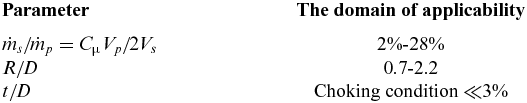
Here, C
μ is the blowing momentum coefficient (in percent) that was described in Equation (1),
 ${R / D}$
is the Coanda surface radius to primary nozzle diameter ratio and t/D is the secondary slot height to primary nozzle diameter ratio. The R
2 value for this regression model was found to be 91.63%, indicating that the model is an accurate representation of the experimental data. Hence, it has the merits of accuracy and comprehensiveness that make it useful as a tool for preliminary sizing. In comparison with the empirical function described by Allen(Reference Allen18), secondary slot height to nozzle diameter ratio is more effective parameter than the control slot arc length over the primary slot circumference. It is worth mentioning that in order to design a fluidic nozzle, the cut-off angle has to be always greater than the maximum predicted thrust deflection angle. Also, as mentioned above, increasing the slot height causes a nonlinear reduction in thrust deflection angle. In fact, increasing the height of the secondary slot for a constant secondary air mass flow rate reduces the momentum, which is the principal parameter in FTV concept and, hence, decreases the thrust deflection angle. In the above function, it is notable that the only geometric parameter that is assumed constant is the primary nozzle diameter, which is dictated by the engine exhaust. The bounds of applicability for the presented formulation, as evidenced by the experimental data are given in Table 3.
${R / D}$
is the Coanda surface radius to primary nozzle diameter ratio and t/D is the secondary slot height to primary nozzle diameter ratio. The R
2 value for this regression model was found to be 91.63%, indicating that the model is an accurate representation of the experimental data. Hence, it has the merits of accuracy and comprehensiveness that make it useful as a tool for preliminary sizing. In comparison with the empirical function described by Allen(Reference Allen18), secondary slot height to nozzle diameter ratio is more effective parameter than the control slot arc length over the primary slot circumference. It is worth mentioning that in order to design a fluidic nozzle, the cut-off angle has to be always greater than the maximum predicted thrust deflection angle. Also, as mentioned above, increasing the slot height causes a nonlinear reduction in thrust deflection angle. In fact, increasing the height of the secondary slot for a constant secondary air mass flow rate reduces the momentum, which is the principal parameter in FTV concept and, hence, decreases the thrust deflection angle. In the above function, it is notable that the only geometric parameter that is assumed constant is the primary nozzle diameter, which is dictated by the engine exhaust. The bounds of applicability for the presented formulation, as evidenced by the experimental data are given in Table 3.
Table 3 The domain of applicability of Equation (3)

The obtained formulation is bounded by the Reynolds numbers for primary and secondary flow and works well for subsonic regimes. The Reynolds numbers are calculated based on the hydraulic diameter (regarding the primary and secondary nozzle diameters) and found to be around 3.67 × 10⁵ for the primary nozzle and 2.21 × 10⁴ for the active secondary channels.
4.0 OPTIMISATION TECHNIQUE
Generally, the optimisation, also known as non-linear programming, is the process of finding the optimum (maximum or minimum) value of a function
 $f(\vec{x})$
as a function of n design variables
$f(\vec{x})$
as a function of n design variables
 $\vec{x} = [{x_1},{x_2},\,.\,.\,.\,,{x_n}]$
in the presence of equality and/or inequality constraints.
$\vec{x} = [{x_1},{x_2},\,.\,.\,.\,,{x_n}]$
in the presence of equality and/or inequality constraints.
In this study, the objective function,
 $f(\vec{x})$
, is defined as thrust vector angle, δ
T
, as shown in Fig. 8.
$f(\vec{x})$
, is defined as thrust vector angle, δ
T
, as shown in Fig. 8.
 $$\begin{equation}
\begin{array}{l@{\quad}l}
f(\vec{x}) = {\delta _T} = atan\left( {{\raise0.7ex\hbox{${{F_Z}\left| {_{_{A - A}}} \right.}$} \!
/ \!\lower0.7ex\hbox{${{F_X}\left| {_{_{A - A}}} \right.}$}}} \right)\\
\qquad\qquad\,\, = atan\left( {\displaystyle\frac{{\int {\rho V{v_z}dA} }}{{\int {\rho V{v_x}dA} }}} \right) \end{array},
\end{equation}$$
$$\begin{equation}
\begin{array}{l@{\quad}l}
f(\vec{x}) = {\delta _T} = atan\left( {{\raise0.7ex\hbox{${{F_Z}\left| {_{_{A - A}}} \right.}$} \!
/ \!\lower0.7ex\hbox{${{F_X}\left| {_{_{A - A}}} \right.}$}}} \right)\\
\qquad\qquad\,\, = atan\left( {\displaystyle\frac{{\int {\rho V{v_z}dA} }}{{\int {\rho V{v_x}dA} }}} \right) \end{array},
\end{equation}$$
where, FX
and FZ
are the components of the thrust force in the X and Z directions, respectively. The design variable vector
 $\vec{x}$
consists of two variables: the Coanda radius and the cut-off angle. The cost function
$\vec{x}$
consists of two variables: the Coanda radius and the cut-off angle. The cost function
 $f(\vec{x})$
should be maximised in a constant blowing momentum coefficient and slot height. The design variables are not dependent and constrained. Therefore, an unconstrained optimisation technique is required. It is worth mentioning that, if the inequality constraint is not active, it does not matter to include it in the calculations. Because the final optimum Coanda radius or cut-off angle is such that the flow is not separated, these constraints are satisfied and not activated within the process. In fact, if the flow is separated, the thrust deflection angle becomes smaller and the maximisation algorithm tries to avoid it.
$f(\vec{x})$
should be maximised in a constant blowing momentum coefficient and slot height. The design variables are not dependent and constrained. Therefore, an unconstrained optimisation technique is required. It is worth mentioning that, if the inequality constraint is not active, it does not matter to include it in the calculations. Because the final optimum Coanda radius or cut-off angle is such that the flow is not separated, these constraints are satisfied and not activated within the process. In fact, if the flow is separated, the thrust deflection angle becomes smaller and the maximisation algorithm tries to avoid it.

Figure 8. Schematic of the forces for definition of thrust vector angle (the objective function).
If the evaluation of a function
 $f(\vec{x})$
is fast, the reasonable method for finding the maximum thrust deflection angle is to evaluate
$f(\vec{x})$
is fast, the reasonable method for finding the maximum thrust deflection angle is to evaluate
 $f(\vec{x})$
for possible
$f(\vec{x})$
for possible
 $\vec{x}$
s. The resulting hypothetical surface is somehow similar to the surface of Fig. 9, as a function of two design variables. Conversely, in this study, finding the cost function for each design point needs CFD simulation that is very slow. Therefore, an optimisation technique, which can find the maximum angle with considerably less simulations is desirable.
$\vec{x}$
s. The resulting hypothetical surface is somehow similar to the surface of Fig. 9, as a function of two design variables. Conversely, in this study, finding the cost function for each design point needs CFD simulation that is very slow. Therefore, an optimisation technique, which can find the maximum angle with considerably less simulations is desirable.

Figure 9. Contours of two-variable objective function.
Most classical non-linear programming methods use the following formula to update the optimum design point
 $\vec{x}$
towards the optimal solution:
$\vec{x}$
towards the optimal solution:
 $$\begin{equation}
{\vec{x}_{i + 1}} = {\vec{x}_i} + \lambda _i^*{\vec{s}_i}
\end{equation}$$
$$\begin{equation}
{\vec{x}_{i + 1}} = {\vec{x}_i} + \lambda _i^*{\vec{s}_i}
\end{equation}$$
Here, the solution starts with an initial guess
 ${\vec{x}_0}$
and stops when a convergence criteria is satisfied. In each step i, a suitable direction
${\vec{x}_0}$
and stops when a convergence criteria is satisfied. In each step i, a suitable direction
 ${\vec{s}_i}$
should be selected, then an appropriate step length λ* must be found in order to improve the solution along the direction
${\vec{s}_i}$
should be selected, then an appropriate step length λ* must be found in order to improve the solution along the direction
 ${\vec{s}_i}$
. To find the search direction, the optimisation methods can be classified into two general categories: direct search methods (also known as non-gradient methods) and indirect search methods (mostly known as gradient-based methods)(Reference Rao23).
${\vec{s}_i}$
. To find the search direction, the optimisation methods can be classified into two general categories: direct search methods (also known as non-gradient methods) and indirect search methods (mostly known as gradient-based methods)(Reference Rao23).
The gradient-based methods benefit from faster convergence. In these methods, the stopping criteria is the norm of the gradient, which should be less than a specified value. In this research, the simplest and most common method in the gradient-based ones known as the steepest descent or Cauchy method is adopted as the optimisation technique. In this technique, the negative of the gradient vector that denotes the direction of steepest descent is used as a search direction,
 ${\vec{s}_i} = - \nabla f({\vec{x}_i})$
. The gradient vector is defined as follows.
${\vec{s}_i} = - \nabla f({\vec{x}_i})$
. The gradient vector is defined as follows.
 $$\begin{equation}
\vec{s} = - \nabla f = - {\left[ {\frac{{\partial f}}{{\partial {x_1}}}\,\,\frac{{\partial f}}{{\partial {x_2}}}\ldots\frac{{\partial f}}{{\partial {x_n}}}} \right]^T}
\end{equation}$$
$$\begin{equation}
\vec{s} = - \nabla f = - {\left[ {\frac{{\partial f}}{{\partial {x_1}}}\,\,\frac{{\partial f}}{{\partial {x_2}}}\ldots\frac{{\partial f}}{{\partial {x_n}}}} \right]^T}
\end{equation}$$
The evaluation of the gradient requires the computation of the partial derivatives. However, the components of the gradient are not available in the case of this study. Therefore, the forward finite difference formula is used to approximate the partial derivatives as follows.
 $$\begin{equation}
{\left. {\frac{{\partial f}}{{\partial {x_i}}}} \right|_{_{{{\vec{x}}_r}}}} = \frac{{f({{\vec{x}}_r} + \Delta \vec{x}) - f({{\vec{x}}_r})}}{{\Delta {x_i}}},\,\,\,\,\,\,i = 1{\ldots}\,n
\end{equation}$$
$$\begin{equation}
{\left. {\frac{{\partial f}}{{\partial {x_i}}}} \right|_{_{{{\vec{x}}_r}}}} = \frac{{f({{\vec{x}}_r} + \Delta \vec{x}) - f({{\vec{x}}_r})}}{{\Delta {x_i}}},\,\,\,\,\,\,i = 1{\ldots}\,n
\end{equation}$$
Here,
 ${\vec{x}_i}$
is the vector of the design variables in the ith iteration,
${\vec{x}_i}$
is the vector of the design variables in the ith iteration,
 ${\vec{x}_r}$
is the vector of reference values and n represents the number of design variables. In practical applications, the value of Δxj
has to be chosen with some care in order to keep the gradient components in the same magnitude of order and prevent any round-off or truncation error.
${\vec{x}_r}$
is the vector of reference values and n represents the number of design variables. In practical applications, the value of Δxj
has to be chosen with some care in order to keep the gradient components in the same magnitude of order and prevent any round-off or truncation error.
The optimisation process using steepest descent technique is shown in Fig. 10. The step length can be fixed or may be found by numerical one-dimensional optimisation methods(Reference Agrawal and Fabien24). Because of the complexity of the current problem and extensive CFD simulations, a fixed step length is selected collaboratively by analysing the results of the initial iterations.

Figure 10. Detailed flowchart of the proposed optimisation technique.
The convergence criterion that one would generally adopt is to stop the procedure whenever the gradient is smaller than a given value (0.1°) or a minimisation cycle produces a change in both variables to be less than one tenth of the required accuracy. When the physical problem is believed to be unimodal (like the case in this study), the convergence is achieved if:
 $$\begin{equation}
f({\vec{x}_{i + 1}}) < f({\vec{x}_i}),\quad {\vec{x}_{i + 1}} \in \{ {\vec{x}_i} \pm \vec{\varepsilon }\}
\end{equation}$$
$$\begin{equation}
f({\vec{x}_{i + 1}}) < f({\vec{x}_i}),\quad {\vec{x}_{i + 1}} \in \{ {\vec{x}_i} \pm \vec{\varepsilon }\}
\end{equation}$$
Unimodality means that there is only one optimum point in the design domain, so the local minimum and global minimum are the same. It is important to note that all unconstrained optimisation methods require a good initial point to start the iterative procedure. This issue is investigated through the author's previous work in this field(20).
5.0 CFD SIMULATION
In the CFD model, the computational grid contains 15 blocks to define the internal passages and the free-stream volume. The computational volume contains the collar surface that extends from the engine exhaust to the far-stream condition. Compared to the nozzle size, this volume is up to 25 times larger in the x direction and 9 times larger in the y and z directions, depending on the engine operating condition. This computational domain is large enough so that the flow dynamics is accounted for and the constraints at the boundaries will not cause any unphysical behaviour. Hence, the final solution will not be affected.
Figure 11 shows the dimensions of the nozzle model. The computational grid as well as the definition of the boundary conditions, making the parametric model for the CFD simulations are also illustrated in Fig. 12. The grid points are set to produce fine mesh close to the walls for the boundary layer, to remain y+ parameter in the limit of the law-of-wall. The area-weighted average for the y+ is found over the entire wall to be around 54.6 that is acceptable for this study. The grid spacing starts at 0.005 mm near the wall and transits smoothly to a relatively coarse mesh. Thus, no wall treatment or adaptation is utilised in the solver. All the blocks are discretised with structured grid and grid dependency is also investigated by verifying the variation of the results from the coarse to the fine grid. Actually, both the control volume and the grid independency checks were performed, based on the authors’ previous experiences by the rectangular and a simple circular nozzles(Reference Banazadeh and Saghafi15,Reference Banazadeh and Saghafi19) . Here, a parameter named meshsize was defined in the journal file (glyph) to automatically change the whole mesh pattern for the independency checks. It was found that a mesh size around 600,000 cells would result in a reasonable response close to the real behaviour and consistent with hardware limitations. Also, control volume was extended 15 to 25 times the nozzle size to get to the best solution. The entire grid system consisted of around 520,000 to 690,000 cells, depending on the size of the collar. The upstream boundary for the primary and the secondary nozzles are set to mass flow-inlet condition, where the primary mass flow rate was calculated from the validated engine performance model by Cranfield's software for Gas Turbine Performance Simulation (known as Turbomatch) for engine speeds ranging from 58,000 to 98,000 rpm(Reference Pachidis25,Reference Ghoreyshi26) . For the purpose of optimisation, this speed is set to 78,000 rpm. The secondary mass flow rate could be adjusted experimentally between 2% and 28% of the primary mass flow rate for each active part. Again, for the purpose of optimisation, this rate is adjusted to 5%. The downstream boundaries are set to pressure outlet condition. The air is also assumed to be ruled by the ideal gas law. The numerical solutions are computed using the well-known finite-volume code FLUENT 6.0 (3d, dp, segregated, ske). In general, an initial prediction of the overall flow conditions could benefit the selection of numerical method and turbulence model. It is assumed that flow is turbulent in the flow-field and regarding the computational cost, both the standard and realisable k-ε models are utilised to study the effects of turbulence in the flow. Accordingly, the segregated solver, with simple pressure-velocity coupling is utilised. Standard pressure and second-order unwinding is used to discretise the convective terms in momentum equations with second-order central differencing used on the viscous terms. The second-order unwinding scheme is also used for energy equation. The iteration process consists of two stages: one for shifting from constant gas properties to ideal gas law after around 3,000 iterations and then, shifting from the first-order to the second-order discretisation to initially converge towards smooth conditions and to achieve better accuracy. It is notable that the convergence of the solution is monitored by checking the residuals of continuity, energy and k-epsilon function to become relatively steady at less than 10E-3 and also evaluating surface integrals of the force terms, Equation (4), that were defined through custom field functions to decay to steady-state values.

Figure 11. Dimensions of the nozzle model and thrust deflection plane.

Figure 12. The computational grid and the main boundary conditions.
The thrust will be deflected in the symmetry plane when the secondary flow is injected from two nearby slots. This plane is also shown in Fig. 11.
Figure 13 shows contours of static temperature and velocity magnitude after 11,000 iterations, indicating that 10.54° of thrust deflection is possible for the basic configuration. Here, the deflection angle is calculated through the surface integration of velocity vectors or momentum on the adjoining plane precisely upon the nozzle in the x and z directions.

Figure 13. Basic nozzle that shows thrust deflection of around 10°. (a) Contours of static temperature and (b) velocity magnitude.
Figure 14 shows the computational grid of the adjoining plane as well as the static temperature contours. Secondary flow and thrust deflection are particularly shown in this view. Validation of the CFD simulation by experimental results and thermal images is presented in references by means of identification and quantification of errors(Reference Banazadeh and Saghafi15,Reference Banazadeh and Saghafi19) . The next part presents how to investigate an optimal geometry for the Coanda surface by the Quasi-Newton optimisation method.

Figure 14. (a) Grid presentation of the adjoining plane and (b) front-view of the static temperature contours in this plane.
6.0 THE RESULTS OF THE OPTIMISATION TECHNIQUE
It is well known in literature that for co-flow fluidic thrust vectoring, the shape of the wall and the relative blowing momentum of fluid, injected through the slots, control the location of the surface stagnation point and therefore the thrust deflection angle. The work undertaken in this research aims to find the best geometry of the Coanda surface in order to maximise the thrust deflection angle. Here, the Quasi-Newton optimisation method in conjunction with CFD simulation is utilised to converge to the best answer. As already mentioned, the formulation is represented for preliminary sizing and is not suitable for optimisation process. Hence, CFD simulation is utilised to optimise for the best deflection angle. Using the proposed optimisation algorithm, after around 51 iterations, the convergence occurs and the answer is found to be satisfactory.
As shown in the optimisation flowchart, the first trial point is taken to have the parameters listed in Table 1, R/D = 1.196, θ = 30°. In the simulation process, regarding the sensitivity analysis, the values for
 $\Delta \vec{x}$
are set to [0.0033, 0.3] in gradient Equation (5). It is noteworthy that when the first trial point is far from the optimum point, the gradient approach produces numbers with very different orders of magnitude and makes the optimisation procedure to drop into a zone, away from the global optimum that needs numerous iterations to converge. The convenient step length was also found to lay between 1 and 100 for every approximation. For example, the first approximation is produced as follows:
$\Delta \vec{x}$
are set to [0.0033, 0.3] in gradient Equation (5). It is noteworthy that when the first trial point is far from the optimum point, the gradient approach produces numbers with very different orders of magnitude and makes the optimisation procedure to drop into a zone, away from the global optimum that needs numerous iterations to converge. The convenient step length was also found to lay between 1 and 100 for every approximation. For example, the first approximation is produced as follows:
 $$\begin{equation*}
\begin{array}{@{}l@{}} f({{\vec{x}}_1})\mathop = \limits^{\mathop \uparrow \limits^{{\rm{CFD Simulation}}} } 10.54^\circ \\ {{\vec{x}}_2} = \mathop {\left[ \begin{array}{@{}l@{}} 1.196\\ 30 \end{array} \right]}\limits_{\mathop \downarrow \limits_{{x_1}} } + \mathop 5\limits_{\mathop \downarrow \limits_{{\lambda ^*}} } \mathop {\left[ \begin{array}{@{}l@{}} \frac{{0.05}}{2}\\[3pt] \frac{{0.11}}{{0.3}} \end{array} \right]}\limits_{\mathop \downarrow \limits_\nabla } = \left[ \begin{array}{@{}l@{}} 1.198\\ 31.8 \end{array} \right]\,\,\,\,\,\,\,\, \Rightarrow \,\,\,f({{\vec{x}}_2})\mathop = \limits^{\mathop \uparrow \limits^{{\rm{CFD Simulation}}} } 10.92^\circ . \end{array}
\end{equation*}$$
$$\begin{equation*}
\begin{array}{@{}l@{}} f({{\vec{x}}_1})\mathop = \limits^{\mathop \uparrow \limits^{{\rm{CFD Simulation}}} } 10.54^\circ \\ {{\vec{x}}_2} = \mathop {\left[ \begin{array}{@{}l@{}} 1.196\\ 30 \end{array} \right]}\limits_{\mathop \downarrow \limits_{{x_1}} } + \mathop 5\limits_{\mathop \downarrow \limits_{{\lambda ^*}} } \mathop {\left[ \begin{array}{@{}l@{}} \frac{{0.05}}{2}\\[3pt] \frac{{0.11}}{{0.3}} \end{array} \right]}\limits_{\mathop \downarrow \limits_\nabla } = \left[ \begin{array}{@{}l@{}} 1.198\\ 31.8 \end{array} \right]\,\,\,\,\,\,\,\, \Rightarrow \,\,\,f({{\vec{x}}_2})\mathop = \limits^{\mathop \uparrow \limits^{{\rm{CFD Simulation}}} } 10.92^\circ . \end{array}
\end{equation*}$$
Figure 15 shows progress of the optimisation process, calculated by the proposed procedure, in 3D space. Continuing the procedure, the best geometry is calculated to be R/D = 1.76, θ = 42°, which makes the optimum thrust deflection angle of 13.97°. This means that the deflection angle is improved by 32%.

Figure 15. Progress of the optimisation process.
Figure 16 illustrates contours of static temperature and velocity magnitude for the optimum geometry. Figure 17 shows the optimum nozzle architecture for the test set-up and a side view that compares between the size and shape of the basic nozzle with the optimum one. In addition, the test results of the optimum nozzle as well as the empirical formulation predictions are shown in Fig. 18, which reveals a close agreement between the analytical Equation (3) and the test results, respectively.

Figure 16. Optimum geometry that shows thrust deflection of 14°. (a) Contours of static temperature and (b) velocity magnitude.

Figure 17. (a) Optimum fluidic nozzle architecture and (b) side view of the basic and optimum fluidic nozzles.

Figure 18. Experimental results versus the correlation function for the optimised fluidic nozzle.
7.0 CLOSING REMARKS
Development of an optimal co-flow fluidic nozzle to deflect the thrust of a small jet engine is presented in this research. Accordingly, the experimentally observed formulation is derived that provides new insight into the parameters that fully govern the co-flow fluidic thrust-vectoring system. The results show significant improvement in about 32% in thrust vector angle for the optimised nozzle over the conventional one. It should be noted that the whole nozzle assembly including the channel, chamber, and flange parts were also redesigned for less size and weight so that the final nozzle assembly is almost half the weight and size of the conventional one.
This study investigated a limited number of configurations to verify the effectiveness of the presented function. Most of the interesting issues between the Coanda shape and thrust-vectoring efficiency have to be investigated in considerably more details as numerous physical aspects are not yet fully understood. This understanding is essential for the implementation and control of this phenomenon for practical applications.
ACKNOWLEDGEMENTS
The authors would like to acknowledge A. Mohajer for his valuable contribution to this research. Also, special thanks go to Dr. M. Ghoreyshi and Dr. N. Assadian for their support and useful suggestions.