


1.0 INTRODUCTION – TYPES OF CFD GRIDS
Structured, unstructured or hybrid grids can be used for CFD calculations. The grids may also use overset or sliding interfaces to account for the relative motion between mesh components or for reducing the complexity of the mesh generation process. In the literature, established helicopter CFD codes( Reference Barakos, Steijl, Badcock and Brocklehurst 1 – Reference Sitaraman, Potsdam, Wissink, Jayaraman, Datta, Mavriplis and Saberi 5 ) have been used with several types of grids without a clear conclusion as to which mesh type is best for computations. In this paper, the idea of hybrid grids is put forward as an attempt to balance accuracy of solution and ease of mesh generation. The basic scheme considered is to keep structured zones where accuracy is required, for example, around the rotor blades or in the rotor wake of a helicopter, and use the unstructured parts to alleviate meshing difficulties in regions with complex geometries, for example, around complex fuselage shapes. Of course, the use of hybrid grids brings forward issues related to the solver (that must cope with different mesh types) and issues related to communication between different mesh types.
The choice of CFD grid type has several consequences beyond the ease of generating a high-quality mesh. These include the computational cost within the CFD solver, the computational storage, and the accuracy and robustness of the employed iterative solution method.
A Cartesian grid is shown in Fig. 1(a). It is a special case of a structured grid where the cells are all squares and aligned with the Cartesian axis system. Such grids are trivial to generate and have faster flux evaluations compared to body fitted grids due to simplified mesh metrics. However, their disadvantage is the complexity in how well boundaries are treated; the cells at a wall boundary are cut by the real geometry of a solid body, which then must be handled via the flow solver.
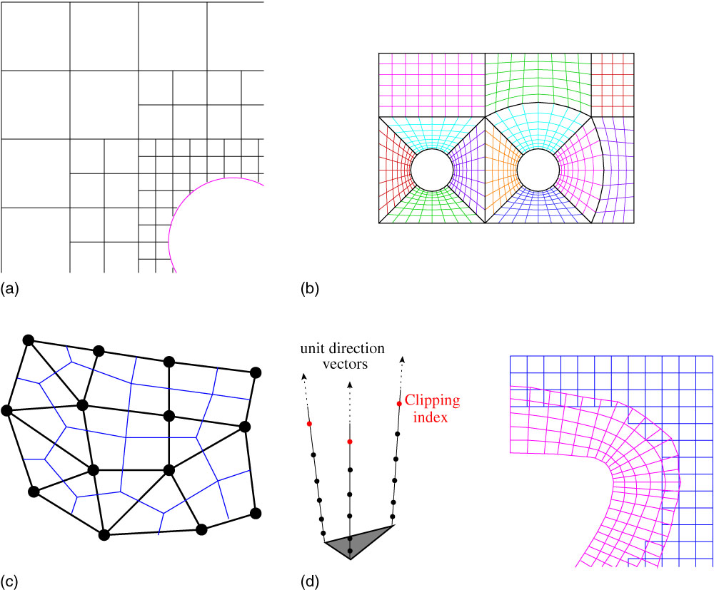
Figure 1 (Colour online) Different types of CFD grids. (a) Cartesian. (b) Multi-block structured. (c) Unstructured. (d) Strand – Cartesian.
A multi-block structured grid, as shown in Fig. 1(b), takes advantage of the flexibility of the unstructured grids in local refinement, and the simplicity and efficiency of structured meshes. In fact, a multi-block mesh can be seen as an unstructured hexahedral mesh. Hence, the advantages of using a body-fitted grid around the geometry can be maintained while reducing the grid generation time.
An unstructured grid, as shown in Fig. 1(c), has an irregular connectivity, and hence, cannot be expressed as a three-dimensional array, meaning it requires more storage, for its connectivity. When a flow has large gradients in one direction with milder ones in the transverse directions like, for example, in boundary-layers, shear layers and wakes, this can lead to highly stretched tetrahedra. This issue is normally overcome by using prism layers in these parts of the flow such that the height of the prism is much smaller than its base.
A strand-Cartesian grid ( Reference Katz, Wissink, Sankaran, Meakin and Chan 6 ) uses a surface mesh and grows ‘strands’ using a smoothed average of the surface normal to produce prismatic cells close to the surface to capture the viscous sub-layer. The smoothing delays the intersection of the strands in concave regions of the surface allowing for longer strands to be used. The off-body mesh is made up of an adaptive Cartesian grid which is refined until its spacing is smaller than the spacing between the points of the strand grid.
It is not just the mesh that is described differently in an efficient solver for a given mesh type. There are different combinations of where the flow solution is stored and what control volumes are used. Even when the grid types use the same schemes, codes will use implied knowledge of the mesh to be more efficient. For examine, if the left and right states of a cell-face are known, the same code could be used to calculate the flux for the Cartesian, multi-block structured and unstructured grids. Admittedly, this would not be very efficient for the Cartesian mesh. However, how the left and right states are calculated would be different between all three versions, and hence the way data are presented to the flux calculating function must be flexible enough to handle them.
There are several techniques for patching multiple grids together, as shown in Fig. 2. One of the methods is the use of non-conformal interfaces between grids. This has been used to a good effect in rotorcraft aerodynamics by embedding the rotor blades into a ‘drum’ which allows movement with respect to the background grid( Reference Steijl and Barakos 2 ). In this case, the use of different point distributions on either side of a curved interface leads to gaps and overlaps, between the rotating drum grid and the stationary background grid. In general, non-conformal interface schemes are only conservative when the interface is planar. The case for the non-conformal interface abutting a curved surface is more problematic since it is possible for the interpolation scheme to use information from the wrong part of the boundary. This issue was addressed in Ref. 7 by mapping the finer grids onto the coarse grid representation of the curve when interpolation coefficients are being calculated between the grids across the interface.

Figure 2 (Colour online) Different patching methods for CFD grids. (a) Sliding planes. (b) DRAGON. (c) Chimera.
Another method allows grids to overlap one another as in the case of chimera or overset methods( Reference Steger, Dougherty and Benek 8 ) already implemented in HMB ( Reference Jarkowski, Woodgate, Barakos and Rokicki 9 ). An extension to this is the DRAGON (Direct Replacement of Arbitrary Grid-Overlapping by Nonstructured) mesh developed by Kao and Liou( Reference Kao and Liou 10 ) which stitches non-overlapping structured meshes for the different components using tetrahedra. DRAGON grids have been extended by Wang et al.( Reference Wang, Qin, Carnie and Shahpar 11 ) into the zipper layer method to increase robustness near small mesh gaps. This was without using an overlap or hanging nodes by adding a small number of tetrahedra and pyramids on either side of the interface to form a conformal mesh.
It is appealing to CFD users and researchers to have a single-code base instead of multiple versions of the same code. However, requirements change over time. The Helicopter Multi-Block (HMB) code( Reference Barakos, Steijl, Badcock and Brocklehurst 1 , Reference Badcock, Richards and Woodgate 12 , Reference Steijl, Barakos and Badcock 13 ), for example, changed from a fixed wing solver to cover rotors, complete helicopters, propellers and wind turbines. The addition of an unstructured mesh capability could be done similarly; however, this would lead to multiple parts of the code doing basically the same thing on different types of mesh. This is undesirable since it leads to code bloat, making it harder to maintain. Also, both versions of the same operations would need to be tested, and any new functionally which can be applied to both mesh types might need to be implemented twice. So the additional functionally of solving on unstructured meshes should be implemented in such a way as to reuse as much of the current code as possible without refactoring it – hence requiring a large re-validation exercise of existing parts of the code.
2.0 HYBRID METHOD IMPLEMENTATION
The goal of any method that uses hybrid grids is to exploit their advantages while minimising their drawbacks. For example, a conformal hybrid mesh can be executed entirely within an unstructured solver with all the extra cost associated with these types of solvers. These drawbacks could be reduced by solving the body-fitted grids using a multi-block structured solver with the remainder domain solved in an unstructured solver. This methodology can be further extended to include a high-order method for solving on Cartesian background grids without having to extend any high-order scheme used for the Cartesian part to the curvilinear grid. Also, it would be possible to solve a different set of governing equations in different parts of the flow. All this functionally is obtained through special treatment of the interface between two different zones, so that each separate solver has all the information required.
The HMB code can solve the discretised Navier–Stokes equations in the integral form using the arbitrary Lagrangian–Eulerian (ALE) formulation( Reference Hirt, Amsden and Cook 14 ) for time-dependent domains with moving boundaries. The equations are discretised using a cell-centred finite volume approach (Fig. 3(a)) on a multi-block grid. Osher’s upwind scheme is used to discretise the convective terms and MUSCL( Reference van Leer 15 ) variable interpolation is used to provide third order accuracy. The Van Albada limiter( Reference van Albada, van Leer and Roberts 16 ) is used to reduce oscillations near steep gradients. Temporal integration is performed using an implicit dual-time step method( Reference Jameson 17 ). The linearised system is solved using the generalised conjugate gradient method with a block incomplete lower-upper (BILU) pre-conditioner. This technique is an iterative method approximating the solution of the linear system using a Krylov subspace method. During iterations, the method requires no matrix–matrix multiplications. Nevertheless, a number of matrix–vector products must be computed. The overhead is only on CPU time, and not so much on the computer memory. Because the matrix–vector products are the most demanding operations of the method, care is taken so these are efficient, and access to the data in memory is optimal. This is the reason frequently in the paper we refer to the cost of the matrix–vector multiplications. Both the Jacobian matrix and the pre-conditioner, which are sparse matrices, are stored in memory. Their formation and solution take around 80% of the computational cost of a fully implicit step with the sparse Jacobian matrix–vector multiplies and pre-conditioner vector multiplies taking nearly 40% of this time. An overview of the parallel implementation of the HMB implicit solver can be found in Ref. Reference Lawson, Woodgate, Steijl and Barakos18.

Figure 3 (Colour online) Two different approaches for control volume (cyan). Bullets indicate placement of flow variables. (a) Cell centred. (b) Vertex centred.
The guiding principle in the implementation of the unstructured functionally of the code was to leverage as much of the existing software as possible to avoid duplication and reduce the cost of validating any newly re-factored functions. This improves the code maintainability while shortening development time since the parts used from an already validated code are much less likely to contain errors. It also reduces the cost of future developments that need to be implemented only once. Like most structured grid codes, HMB was written assuming the mesh had a certain connectivity to increase performance at the expense of generality and so functions had to be extended to allow for greater flexibility in the input arguments while not changing the returned variables when called from structured blocks. Another consideration is that any extra functionally needed for the new implementation be useable with a structured multi-block mesh. For example, the new method for calculating gradients at the centroid of the cells needed for the unstructured mesh should also be used within a structured multi-block mesh.
The Helicopter Unstructured Method (HUM) functionally has been implemented using a similar scheme to HMB albeit with some differences. First, the governing equations are discretised using a vertex-based approach (Fig. 3) on the unstructured mesh. Hence, the solution unknowns are stored at the grid points instead of the cell centres and the cell control volume is now obtained using the dual mesh. With structured grids, the second neighbours of each cell are well defined and these are used in the spatial discretisation of the equations (e.g., in the MUSCL scheme). With unstructured grids, this is not the case, and flow gradients are used instead to the same effect. The remainder of the functionally is the same but due to the differences outlined above, a structured multi-block mesh will not produce perfectly identical results when run using the unstructured mode.
There were several reasons behind choosing a vertex-based approach for the unstructured mesh vs the cell-centred-based approach for the structured mesh. First, in unstructured meshes, there are many more cells than vertices and keeping the number of field variables as low as possible is advantageous for parallel computations. Changing the position of the unknowns does not affect the assembly of the Jacobian matrix and only slightly affects its parallel solution since the matrix–vector multiplications need different functions to exchange solution data. This is the case because HMB currently partitions a multi-block mesh without sub-division of the blocks. Between structured and unstructured grids, the loops that build the cell residuals need to be different but the flux calculation through a face, and source term calculations are the same. For example, in HMB, the cell volumes are used, while in HUM, the dual mesh volume is employed. One difference in the code is how the boundaries of the blocks are calculated. HMB uses two layers of halo cells around each block for consistent calculation of the fluxes shared between two blocks while HUM exchanges a single row of solutions and gradients on the block boundaries, to accomplish the same task. Physical boundaries are also treated differently since halo cells are used to set the boundary conditions in HMB while the boundaries are enforced directly through the flux on the boundary within HUM. The calculation of the mesh metrics is also different because of the different ways the meshes are stored. Some key aspects of the unstructured/structured implementation are now detailed.
2.1 Data structure
The extension of the multi-block data structure requires extra information in defining the mesh and edge data. First, an unstructured block requires more information to be fully defined compared to a block of a structured mesh since there is no implicit ordering. Looking at Fig. 4, a structured mesh with a grid of n x × n y × n z cells is used as an example. Given any cell i, j, k, the eight nodes making up this cell are known implicitly and can be accessed in a three-dimensional array or mapped into a one-dimensional array as in the case of HMB. Hence, information about the connectivity does not need to be stored. In an unstructured block format, for a given cell, it is impossible to write a simple mapping function that recovers the eight nodes. This issue is resolved with the use of element data, which contain all the nodes making up the vertices of the element. There are many different types of elements with the four common ones being, tetrahedra, prisms, pyramids and hexahedra. To reduce the complexity of the data structure, instead of performing operations on each element type the elements are decomposed into unique edges. These edges consist of the two end points i and j. The vector x j −x i , and the normal and surface data of the control volume of the edge need to be computed and stored. It should be noted that after the edge data have been calculated along with the dual volumes, the element data can be discarded. The edge data are very important within an unstructured solver because most operations are loops over the edges. Selmin and Formaggia( Reference Selmin and Formaggia 19 ) amongst others presented a framework for constructing node-centred schemes and defined a flexible data structure for meshes with different element types which consisted of node pairs linking two grid points together. A final important performance aspect is how the nodes and edges are numbered. Currently, the nodes are grouped into six different types as shown in Fig. 5(a). The vast majority are interior nodes (circles), and interior boundary nodes (squares) that are all the nodes which can be fully updated when using a first-order scheme without communication. The remainder are nodes that are updated on the current processor (up and down triangles) and halo nodes (diamonds and crosses) that are updated on other processors. Even though the node marked by a cross in Fig. 5(a) is not required for the residual evaluation, it has been included to allow for the calculation of element-based data if required for post-processing.

Figure 4 (Colour online) Cell and node numbering for a structured and an unstructured mesh.

Figure 5 (Colour online) The node and edge numbering schemes. (a) Types of nodes. (b) Internal edges (block). (c) External edges (block).
Grouping the nodes in this way implies that all rows of the first-order Jacobian matrix that require data from another processor to perform a matrix–row vector multiplication are at the end of the arrays used in the code. No extra logic is required to reorder the operations for parallel matrix–vector multiplications so that all the rows containing just local data can be calculated first. This allows the messages exchanged between CPUs for parallel calculations to be split with the local operations carried out in between them to hide some of the communication overhead. The following steps are used:
∙ Send the data to the other processors.
∙ Perform the local part of the matrix–vector multiplication – the vast majority of it.
∙ Receive the data needed for the remainder of the rows.
∙ Finish the non-local part of the parallel matrix–vector multiplication.
There are two different types of edges: first edges where both end points are updated, Fig. 5(b), and, second, edges that only update one end, Fig. 5(c). In the case where only one edge point needs to be updated, it is always the i point that needs updating and never the j, Fig. 5(a). These two groups of edges are then split into subgroups. The internal edges are split into three groups shown in Fig. 5(b) and the external edges are split into four different groups shown in Fig. 5(c). These groups differentiate between the types of nodes which make up the end points of the edges. The largest group is when both ends of an edge are interior nodes (circles). The reason behind splitting the edges into subgroups is the same as the numbering of the nodes. It allows the parallel flux calculations to be split into local and non-local parts where both the local internal and boundary fluxes can be computed while the data exchange is carried out.
Since the structured multi-block mesh uses an approximate Riemann solver which requires the left and right states, a normal vector and a cell-face area, the information stored in the edge data is exactly equivalent except for where the information is stored.
2.2 Gradient calculation
A good approximation for the gradient of the solution is imperative in CFD solvers. For example, in the Navier–Stokes equations, the viscous flux functions contain gradients of both velocity components and temperature. Two standard methods have been implemented for their computation using either the Gauss–Green approximation or weighted least squares. The Gauss–Green approximation appeals to the divergence theorem, which states that the outward flux of a vector field through a closed surface is equal to the volume integral of the divergence over the volume inside the surface. This is stated as
 $$\mathop{\int}_V {(\nabla \cdot U){\rm d}V} {\equals}\mathop{\oint}_S {(U \cdot n){\rm d}S} $$
where U is a continuously differentiable vector field, and V is a volume bounded by the surface S with an outward pointing normal n. The integral mean value theorem to obtain the gradient at the centre of the volume V using
 $$U_{x} {\equals}{1 \over V}\mathop{\oint}_S {U(x,y){\rm d}y} $$
were the right-hand side of (2) is evaluated with a quadrature rule. For vertex-based schemes, V is the dual control volume and then the mid-point rule is used for the quadrature scheme. This leads to a scheme that is exact for linear functions on tetrahedral grids.
The least squares gradient calculation( Reference Mavriplis 20 ) is a method unrelated to the mesh topology. Its construction only needs a set of neighbouring points close to the position where the gradient is to be calculated. Even though any stencil is possible, the normal construction for a vertex based scheme is to take all the neighbouring points which are connected via an edge. These are the same points that would be used to calculate the first-order inviscid flux. The least squares gradient is then obtained by solving for the values of the gradient which minimise the sum of the squares of the differences between neighbouring values.
The least squares gradient calculation gives an exact gradient for a linear variation of the variable, while for the Gauss–Green reconstruction, this does not hold for all grid types. However on thin cells with large curvature, like boundary-layer meshes for high Reynolds number flows, the least squares gradient can give erratic results( Reference Mavriplis 20 ) compared to Gauss–Green. Therefore, different gradient calculations are suitable for different cell types.
2.3 Limiting the solution
Barth and Jespersen( Reference Barth and Jespersen 21 ) were the first to introduce a limiter for unstructured grids. The idea was to find a value of ϕ in each control volume which would limit the gradient in the reconstruction of the solution u so that the interface does not produce local maxima or minima. The scheme reads
 $$u_{{ij}} {\equals}u_{j} {\plus}\rphi _{i} \nabla u_{i} .{{x_{j} {\minus}x_{i} } \over 2},\quad \rphi _{i} \in[0,1]$$
where
 $$\nabla u_{i} {\equals}\left( {{{\partial u_{i} } \over {\partial x}},{{\partial u_{i} } \over {\partial y}},{{\partial u_{i} } \over {\partial z}}} \right).$$
The non-differentiability of this limiter adversely affects the convergence properties of the solver. Due to this, Venkatakrishnan( Reference Venkatakrishnan 22 ) introduced a smooth alternative to the Barth–Jespersen procedure, as well as, a parameter to turn the limiter off in smooth regions of the flow. However, the authors found that at stagnation points, where the gradient of the solution changes sign, this limiter still causes convergence problems unless the tunable parameter is set so large that it turns the limiter off over the whole mesh.
In the current work, a different formulation is used which more closely resembles the limiter used in the multi-block HMB. HMB approximates the left and right states by interpolation of a second-order, upwind biased, difference equation which results in a parabolic reconstruction scheme. The scheme reads
 $$u_{{i{\plus}1\,/\,2}}^{L} {\equals}u_{i} {\plus}{{\rphi (r_{i} )} \over 4}\left[ {(1{\minus}\chi ){\rm \Delta }_{{\minus}} u_{i} {\plus}(1{\plus}\chi ){\rm \Delta }_{{\plus}} u_{i} } \right]$$
where Δ+ u i =u i+1−u i , Δ− u i =u i −u i−1, ϕ(r i ) is the limiter and r i =Δ− u i /Δ+ u i . If ϕ(r i )=0, then this is only a first-order scheme but if ϕ(r i )=1 then a family of higher order schemes is achieved which are at least second order for all values of −1≤χ≤1. HMB uses the alternative form of the van Albada limiter namely
 $$\rphi (r){\equals}{{2r} \over {r^{2} {\plus}1}}.$$
It should be noted that this limiter is not second-order TVD since for any r ∈(1, 2), ϕ(r)<1. The value of χ is set to zero giving the final formulation:
 $$u_{{i{\plus}1\,/\,2}}^{L} {\equals}u_{i} {\plus}{{{\rm \Delta }_{{\minus}} {\rm \Delta }_{{\plus}} } \over {2({\rm \Delta }_{{\plus}}^{2} {\plus}{\rm \Delta }_{{\minus}}^{2} )}}\left[ {{\rm \Delta }_{{\minus}} {\plus}{\rm \Delta }_{{\plus}} } \right].$$
To be able to reuse this formulation in unstructured grids the difference Δ− u i =u i − u i−1 needs to be replaced since the second neighbour u i−1 is not well defined. The approximation
 $$u_{i} {\minus}u_{{i{\minus}1}} \,\approx\,2.0\nabla u_{i} \,\cdot\,(x_{j} {\minus}x_{i} ){\minus}(u_{j} {\minus}u_{i} )$$
is used, and Equation (5) can then be used to calculate the left state in both structured and unstructured cases.
2.4 Flux calculation
The flux calculation for a cell is constructed by summing all fluxes through the faces that make up the cell. In HMB, this is done using two loops over the faces. The first is for inviscid and the second for vicious. For the inviscid loop, the left and right limited flow states are calculated and then the approximate Riemann solver calculates the flux through the face. Only the solution of the two points either side of the edge are used as shown in Fig. 6. The viscous flux requires an approximation of both the solution and the gradient at the centroid of the face. The solution is averaged from the two neighbouring cells while the gradient is calculated using Gauss–Green around the control volume shown in Fig. 6(b). This leads to six points being used in the calculation of the viscous flux for each face. The final is a 13 point stencil in two dimensions, shown in Fig. 6(c) or a 25 point stencil in three dimensions.

Figure 6 (Colour online) The flow variables used to calculate the HMB flux. Blue inviscid, red viscous and black (both). (a) Inviscid face. (b) Viscous face. (c) Full stencil.
In HUM, the inviscid and viscous flux terms are added in a single operation for great computational efficiency. The left and right limited flow states are calculated using Equations (5) and (6) increasing the size of the inviscid stencil because the gradients of the solution are also required. Since the gradients are required for both the inviscid and viscous fluxes, the flux through an edge has exactly the same 8 point stencil as shown in Fig. 7. The gradient calculation at the midpoint of the edge is done by the corrected average method that uses the average of the gradients at the end points of the edge, then removes the component of the gradient along that edge ij and replaces it with its central difference. This removes any undesirable odd–even decoupling and also reduces the size of the stencil on certain types of meshes. As can be seen from Figs 6 and 7, the viscous stencil on hexahedral meshes is the same for HMB and HUM.

Figure 7 (Colour online) The flow variables used to calculate the HUM flux. (a) Inviscid and viscous. (b) Full stencil.
2.5 Coupling methods
The method for coupling a block-structured zone to an unstructured depends on the restrictions placed on the interface( Reference Vanharen, Puigt and Montagnac 23 ). The most restrictive case is the one where the interface is required to be conformal. An example of a conformal interface is shown in Fig. 8(a). An interface is conformal if both points and edges coincide for each zone. This can either be achieved by splitting the face on the block-structured side and calculating the flux on each triangle, or by using a layer of pyramids on the unstructured side to transition into the tetrahedral mesh. The latter case was implemented. Block-structured zones have two rows of ‘halo’ cells, to keep the calculation of the fluxes on the interface consistent between block interfaces. This can only be achieved if the mesh on both sides of the interface is also the same. To be able to do this at the interface between a block structured and an unstructured zone, puts a restriction that the first two layers cells must be hexahedra as shown in Fig. 8(d).
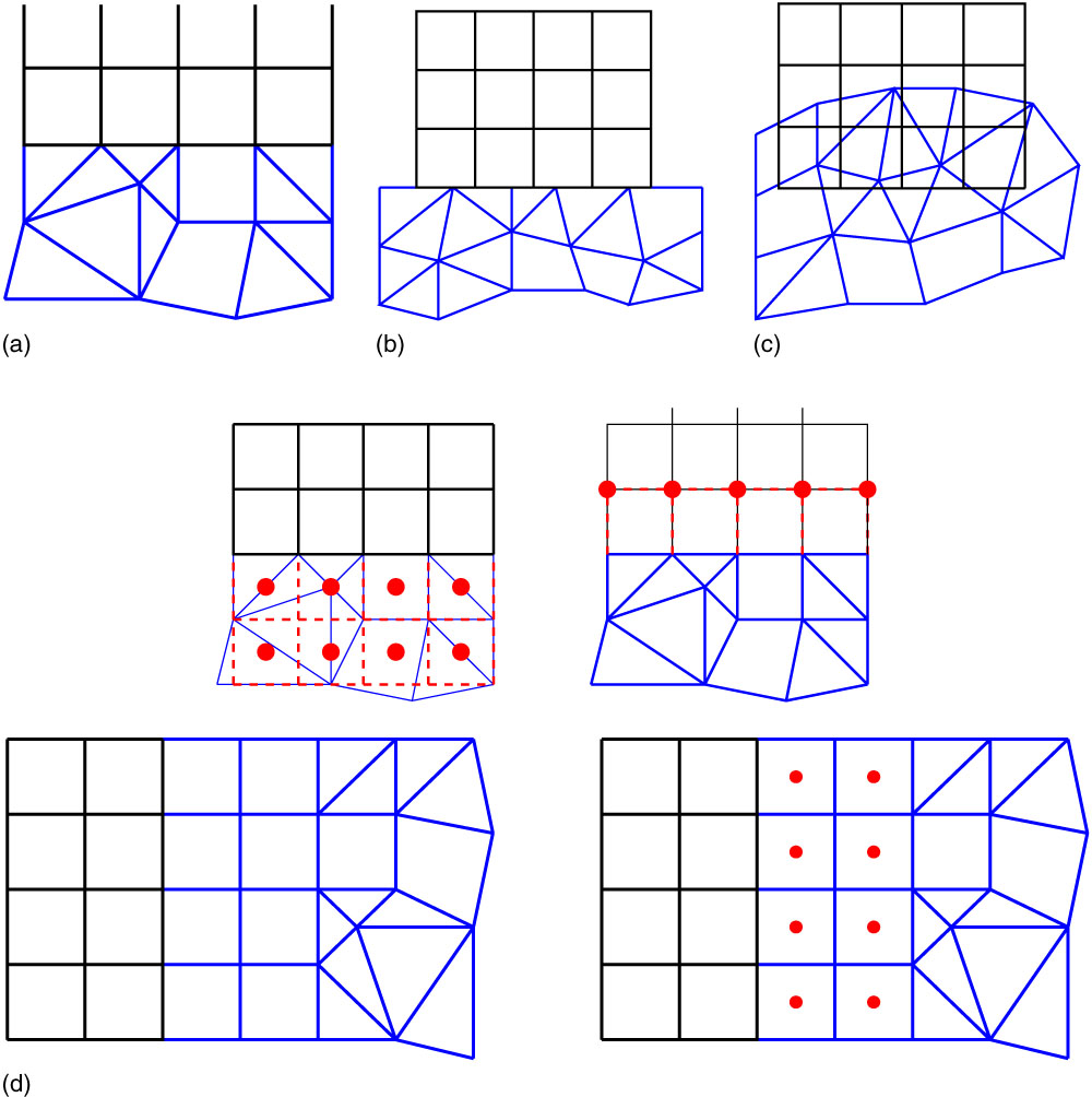
Figure 8 (Colour online) Different coupling methods and interpolation strategies. (a) Conformal patching. (b) Non-conformal patching. (c) Fully non-matching. (d) Interpolation strategy with a double layer of hexahedrons in the unstructured grid.
A slightly less restrictive case is the one where the two interfaces coincide but the points do not. This is shown in Fig. 8(b). If the interface is curved, this also leads to having both holes and overlaps in the mesh. This can be greatly reduced if the same density of points is used on both sides of the interface. Another option would be to pre-process the grid by projecting the higher density interface onto the lower with a method similar to the one described in Ref.Reference Woodgate and Barakos7.
The least restrictive case is that of going to non-matching interfaces and using an overset grid. It should be noted that not all the functionally of a chimera method would be required if, for example, the grids were built in such a way that no hole cutting is needed. In this case, for block structured zones, both rows of halo cells must be interpolated from the overlapping mesh. An unstructured zone would require the solution and gradients for all points on the outer boundary to be interpolated from another zone.
3.0 IMPLICIT FLOW SOLVER
The Navier–Stokes equations can be discretised using a finite volume approach. The computational domain is divided into a finite number of non-overlapping control-volumes, and the governing equations are applied to each cell in turn. The spatial discretisation of the NS equations leads to a set of ordinary differential equations in time
 $${{\rm d} \over {{\rm d}t}}\left( {{\bf W}V} \right){\equals}{\minus}{\bf R}\left( {\bf W} \right).$$
where W and R are the vectors of cell conserved variables and residuals, respectively, and V is the cell volume. Using a fully implicit time discretisation and approximating the time derivative by a second-order backward difference Equation (7) becomes
 $${{3V^{{n{\plus}1}} {\bf W}^{{n{\plus}1}} {\minus}4V^{n} {\bf W}^{n} {\plus}V^{{n{\minus}1}} {\bf W}^{{n{\minus}1}} } \over {2{\rm \Delta }t}}{\plus}{\bf R}({\bf W}^{{n{\plus}1}} ){\equals}0.$$
Equation (8) is non-linear in W n+1 and cannot be solved analytically. This equation is defined to be the unsteady residual R *. Following the original implicit dual-time approach introduced by Jameson( Reference Jameson 17 ), Equation (8) is solved by iteration in pseudo-time t *. This permits the acceleration techniques of steady-state flow solvers to be used to obtain the updated solution and allows the real time step to be chosen based on accuracy requirements alone without stability restrictions. Using an implicit time discretisation on the pseudo-time t *, we can write
 $${{{\bf W}^{{m{\plus}1}} {\minus}{\bf W}^{m} } \over {{\rm \Delta }t^{{*}} }}{\equals}{\minus}{{{\bf R}^{{*}} ({\bf W}^{{m{\plus}1}} )} \over {V^{n} }}$$
where the superscript m + 1 denotes the level
 $(m{\plus}1){\rm \Delta }t^{{*}} $
in pseudo-time. In this equation, the flux residual on the right-hand side is evaluated at the new time level m + 1 and is, therefore, expressed in terms of the unknown solution at this new time level. The unsteady flux residual
$(m{\plus}1){\rm \Delta }t^{{*}} $
in pseudo-time. In this equation, the flux residual on the right-hand side is evaluated at the new time level m + 1 and is, therefore, expressed in terms of the unknown solution at this new time level. The unsteady flux residual
 ${\bf R}^{{*}} \left( {{\bf W}^{{m{\plus}1}} } \right)$
is linearised in the pseudo-time variable
${\bf R}^{{*}} \left( {{\bf W}^{{m{\plus}1}} } \right)$
is linearised in the pseudo-time variable
 $t^{{*}} $
as follows:
$t^{{*}} $
as follows:
 $$\openup3pt\matrix{ {{\bf R}^{{*}} ({\bf W}^{{m{\plus}1}} )} \hfill &\hskip-8pt {\equals} \hfill & \displaystyle\hskip-9pt{{\bf R}^{{*}} ({\bf W}^{m} ){\plus}{{\partial {\bf R}^{{*}} } \over {\partial t^{{*}} }}{\rm \Delta }t^{{*}} {\plus}O({\rm \Delta }t^{{{*}2}} )} \hfill \cr {} \hfill & \hskip-8pt\,\approx\, \hfill &\hskip-9pt \displaystyle{{\bf R}^{{*}} ({\bf W}^{m} ){\plus}{{\partial {\bf R}^{{*}} } \over {\partial {\bf W}}}{{\partial {\bf W}} \over {\partial t^{{*}} }}{\rm \Delta }t^{{*}} } \hfill \cr {} \hfill &\hskip-8pt \,\approx\, \hfill & \displaystyle\hskip-9pt{{\bf R}^{{*}} ({\bf W}^{m} ){\plus}{{\partial {\bf R}^{{*}} } \over {\partial {\bf W}}}{\rm \Delta }{\bf W},} \hfill \cr } $$
where ΔW=W m+1 − W m , and by using the definition of the unsteady residual:
 $${{\partial {\bf R}^{{*}} } \over {\partial {\bf W}}}{\equals}{{\partial {\bf R}} \over {\partial {\bf W}}}{\plus}{{3V} \over {2\Delta t}}{\bf I}.$$
Substituting the above in Equation (9) and rewriting in terms of the primitive variables P we obtain
 $$\left[ {\left( {{V \over {{\rm \Delta }t^{{*}} }}{\plus}{{3V} \over {2{\rm \Delta }t}}} \right){{\partial {\bf W}} \over {\partial {\bf P}}}{\plus}{{\partial {\bf R}} \over {\partial {\bf P}}}} \right]{\rm \Delta }{\bf P}{\equals}{\minus}{\bf R}^{{*}} ({\bf W}^{m} ).$$
where ∂R/∂P is the Jacobian matrix. This is the basic time-marching equation employed in both HMB and HUM.
3.1 Jacobian matrix
The properties of the Jacobian matrix have a strong influence on the performance of this scheme. An exact Jacobian matrix recovers Newton’s method, if
 ${\rm \Delta }t^{{*}} $
is very large, giving quadratic convergence when close enough to the final solution. However, the exact Jacobian is very stiff for high Reynolds number flows making it very hard to solve Equation (12) as well as having a very narrow domain where the solution converges. To make the solver more robust, the matrix is approximated. This increases the number of iterations to obtain convergence but is counteracted by the approximate Jacobian being less stiff, having fewer non-zero terms. So Jacobian vector operations are faster, and Equation (12) only needs to be approximately solved.
${\rm \Delta }t^{{*}} $
is very large, giving quadratic convergence when close enough to the final solution. However, the exact Jacobian is very stiff for high Reynolds number flows making it very hard to solve Equation (12) as well as having a very narrow domain where the solution converges. To make the solver more robust, the matrix is approximated. This increases the number of iterations to obtain convergence but is counteracted by the approximate Jacobian being less stiff, having fewer non-zero terms. So Jacobian vector operations are faster, and Equation (12) only needs to be approximately solved.
An approximate Jacobian ∂W/∂U is used to reduce the sparsity pattern of the Jacobian matrix as well as the stiffness of the linear system. The Jacobian matrix is calculated analytically by repeated application of the chain rule. The residual for one cell is built up as a summation of the fluxes through the cell faces. The inviscid part of the residual of the cell face is, denoted by f i−1/2 in Fig. 9, and follows the usual approach for Riemann solvers:
 $$f_{i _{{{\minus}1\,/\,2}}} {\equals}f_{i _{{{\minus}1\,/\,2}}} \left( {U_{L} ,U_{R} } \right)$$
where U L and U R are the left and the right states, respectively, of the Riemann problem. Applying the MUSCL would result in four contributions to the Jacobian matrix arising from
 $${{\partial f_{{i{\minus}1\,/\,2}} } \over {\partial U_{{i{\minus}2}} }}, \qquad{{\partial f_{{i{\minus}1\,/\,2}} } \over {\partial U_{{i{\minus}1}} }}, \qquad{{\partial f_{{i{\minus}1\,/\,2}} } \over {\partial U_{i} }}, \qquad{{\partial f_{{i{\minus}1\,/\,2}} } \over {\partial U_{{i{\plus}1}} }}.$$

Figure 9 Points used in the calculation of the one-dimensional residual of the cell i.
To reduce ill-conditioning, the exact Jacobian matrix is approximated by removing this dependence by the following approximation:
 $${{\partial f_{{i{\minus}1\,/\,2}} } \over {\partial U_{{i{\minus}2}} }}\,\approx\,0,\; \qquad{{\partial f_{{i{\minus}1\,/\,2}} } \over {\partial U_{{i{\minus}1}} }}\,\approx\,{{\partial f_{{i{\minus}1\,/\,2}} } \over {\partial U_{L} }}, \;\qquad{{\partial f_{{i{\minus}1\,/\,2}} } \over {\partial U_{i} }}\,\approx\,{{\partial f_{{i{\minus}1\,/\,2}} } \over {\partial U_{R} }}, \;\qquad{{\partial f_{{i{\minus}1\,/\,2}} } \over {\partial U_{{i{\plus}1}} }}\,\approx\,0.$$
This scheme is similar to calculating the exact Jacobian matrix for a first-order spatial discretisation, with the modification that the MUSCL interpolated values at the interface are used in the evaluation instead of the cell values that would be used for a first-order spatial scheme. It is highly desirable not to expand this non-zero pattern when adding in the viscous terms to the Jacobian. For viscous fluxes, a thin shear layer approximation is used when forming the Jacobian terms which only takes into account the gradient vectors normal to the face.
In the multi-block structured case, this approximate Jacobian has seven non-zero entries per row. In the unstructured case for a hexahedral mesh, this is still true since each vertex has six edges. However, for a general unstructured mesh using a vertex-centred scheme, this will increase. For example, Fig. 10 shows a histogram of the number of edges per point for the ERICA fuselage case of Section 4.4. Most have nine non-zero terms per row since this occurs from prisms which are grown from a surface mesh where six triangles meet at a point. The average number of terms per row, in this case, is 10.52 with six rows having 24 non-zero terms. This increase from 7 to 10.5 raises the computational cost of a matrix–vector multiplication by 50%. The cost is further increased due to the non-fixed distance between the columns of any given row, which means more access to computer memory. Since a sparse matrix–vector multiplication is memory bandwidth limited( Reference Goumas, Kourtis, Anastopoulos, Karakasis and Koziris 24 ), anything that increases loads from computer memory reduces the performance.

Figure 10 (Colour online) Histogram of the number of non-zero per row in the approximate Jacobian matrix for a 5.3 m node unstructured Erica fuselage mesh used in Section 4.4.
3.2 Linear solvers
There are two methods available for solving the linear system in HMB/HUM. The first is a Krylov subspace algorithm. Eisenstat, Elman and Schultz( Reference Eisenstat, Elman and Schultz 25 ) developed a generalised Conjugate Gradient method that depends only on A rather than A T A called the Generalised Conjugate Residual (GCR) algorithm. Further, Saad and Schultz( Reference Saad and Schultz 26 ) developed the Generalised Minimal Residual (GMRES) algorithm which is mathematically equivalent to GCR but is less prone to breakdown for certain problems and requires less storage and arithmetic operations. However, GCR remains the easier algorithm to implement especially in parallel. The GCR algorithm in HMB is preconditioned using a block incomplete lower upper (BILU) factorisation( Reference Axelsson 27 ).
The second linear solver is based on splitting the Jacobian matrix into the lower diagonal and uppers parts
 $$A{\equals}L{\plus}D{\plus}U{\equals}\left( {L{\plus}D} \right)D^{{{\minus}1}} \left( {U{\plus}D} \right){\minus}LD^{{{\minus}1}} U$$
where L only consists of block terms which are strictly below the diagonal, U only consists of block terms which are strictly above the diagonal and D is a block diagonal matrix. If assumed that the LD −1 U is negligible, the following equation can be used to solve for the solution update:
 $$(L{\plus}D)D^{{{\minus}1}} (U{\plus}D){\rm \Delta }{\bf W}^{n} {\equals}{\minus}{\bf R}({\bf W}^{n} ).$$
Equation (13) can be inverted by using a forward and backward sweeps procedure:
 $$\left\{ {\matrix{ {D{\rm \Delta }{\bf W}^{{*}} {\equals}{\minus}{\bf R}({\bf W}^{n} ){\minus}L{\rm \Delta }{\bf W}^{{*}} } \hfill \cr {D{\rm \Delta }{\bf W}^{n} {\equals}D{\rm \Delta }{\bf W}^{{*}} {\minus}U{\rm \Delta }{\bf W}^{n} } \hfill \cr } } \right.$$
where
 ${\rm \Delta }{\bf W}^{{*}} $
is the solution vector updated in the forward sweep. There are a number of ways to set up the Jacobian matrix. In the original LU-SGS scheme, the matrix is constructed based on splitting the inviscid flux Jacobian according to its spectral radius. This treatment reduces the computational complexity of the scheme and ensures the matrix is diagonally dominant (
Reference Yoon and Jameson
28
,
Reference Chen and Wang
29
). However, in the case of HMB/HUM, the Jacobian matrix is the same as the one used in Section 3.1. This means that the memory required to store the preconditioner and the generalised conjugate residual solver bases are not required. This is at the expense of taking more iterations to solve the linear system, and usually, a lower CFL number is needed to keep the system more diagonally dominant.
${\rm \Delta }{\bf W}^{{*}} $
is the solution vector updated in the forward sweep. There are a number of ways to set up the Jacobian matrix. In the original LU-SGS scheme, the matrix is constructed based on splitting the inviscid flux Jacobian according to its spectral radius. This treatment reduces the computational complexity of the scheme and ensures the matrix is diagonally dominant (
Reference Yoon and Jameson
28
,
Reference Chen and Wang
29
). However, in the case of HMB/HUM, the Jacobian matrix is the same as the one used in Section 3.1. This means that the memory required to store the preconditioner and the generalised conjugate residual solver bases are not required. This is at the expense of taking more iterations to solve the linear system, and usually, a lower CFL number is needed to keep the system more diagonally dominant.
3.3 Actuator disk models
The actuator disk simulates the effect of a rotor by creating a pressure difference on a single plane inside the flow field. This is a useful and fast method when simulating the flow around a fuselage where the focus is more on the fuselage than on the rotor blades. Uniform and non-uniform actuator disk models have been implemented and are shared between HMB/HUM.
3.3.1 Uniform actuator disk
An actuator disk adds a source term to the momentum and energy equations to impose the pressure difference ΔP across the rotor disk which depends on the advance ratio μ and thrust coefficient C T . In the uniform case, the non-dimensional pressure difference ΔP * is given by
 $${{C_{T} } \over {\rmu ^{2} }}{\equals}{T \over {\rrho _{\infty} V_{{{\rm tip}}}^{2} A\rmu ^{2} }}{\equals}{{{\rm \Delta }P} \over {\rrho _{\infty} V_{{{\rm tip}}}^{2} }} \cdot {{V_{{{\rm tip}}}^{2} } \over {V_{\infty}^{2} }}{\equals}{{{\rm \Delta }P} \over {\rrho _{\infty} V_{\infty}^{2} }}{\equals}{\rm \Delta }P^{{\asterisk}} $$
where T is the rotor thrust, V tip is the velocity at the rotor tip, ρ∞ is the freestream density, V ∞ is the freestream velocity and A is the area of the rotor disk.
3.3.2 Non-uniform actuator disk
In forward flight, the rotor load distribution is not uniform and a more realistic actuator disk model should give the pressure jump as a function of the radial position on the blade r and the azimuth angle Ψ. Shaidakov’s AD model( Reference Shaidakov 30 ), expresses the loading of a forward flying rotor with a distribution of the form
 $${\rm \Delta }P^{{\asterisk}} {\equals}P_{0} {\plus}P_{{1S}} \:{\rm sin}({\rm \Psi }){\plus}P_{{2C}} \:{\rm cos}(2{\rm \Psi }),$$
where the coefficients P 0, P 1S and P 2C depend on rotor radius and solidity, rotor attitude, advance ratio, thrust coefficient, lift coefficient slope and free-stream velocity. The model accounts for blade tip offload, and the reversed flow region, as well as the rotor hub. Details of Shaidakov’s model can be found in Refs 30, and 31. The model originates from the theory of an ideal lifting rotor in incompressible flow and it has been tuned for realism using flight tests data. A detailed description of the model's implementation in HMB can be found in Ref.Reference Chirico, Szubert, Vigevano and Barakos32.
3.4 Parallel implementation
The parallel implementation of the Helicopter Unstructured Method (HMB/HUM) is done through partitioning the domain into smaller pieces using METIS( Reference Karypis and Kumar 33 ). This is a fast process taking less than a 20 s for a mesh of 3.5 m cells. Since the process is linear in the number of cells, partitioning meshes of even 100 m cells are not CPU limited. The limiting factor is the amount of memory needed. This again is linear in the number of cells and currently 1 m cells require 720 MBytes of memory. Hence, a 100 m cell mesh would take around 10 min of CPU time but also around 70 GBytes of memory.
Since the grid has been partitioned into multiple domains, information must be exchanged between processors. Unlike the structured solver in which a double row of halo cells is exchanged the unstructured solver needs a single row of both the solution and its spatial gradients to calculate the residual. This is twice the amount of information since the gradients require three times the information, and the gradient of the temperature is also communicated in addition to the gradients of density, velocity, pressure and the quantities related to the turbulence models.
Due to the use of a first-order Jacobian matrix, both solvers require a single-row data to perform a matrix–vector multiplication in parallel and are only stored as floats (4 Bytes). The reduction in accuracy of using floats is negligible compared to the difference between the exact and approximate Jacobian. Since the matrix is stored in this way, the communication size is further decreased by reducing the precision from 8 Bytes per variable to 4. It should be noted that all the inner products in the GCR method must still be stored in 8 Bytes so as to delay the degradation in the orthogonalisation for the search directions.
3.5 Parallel performance
Modern central processing units (CPUs) have large numbers of cores. At present, high-performance computing nodes commonly have two CPUs each with 16–24 cores per CPU. This means that good code efficiency across many thousands of cores requires two different types of parallel performance: (a) within a compute node, and (b) across compute nodes. Within a node, messages use a shared-memory byte transfer layer which is a local memory copy and is much faster than the interconnect between nodes. Nodes though have a fixed amount of cache, memory bandwidth. Between nodes, the messages will be sent over the interconnect, which is slower, but the amount of resources also scales linearly with the number of nodes. This leads to two very different scaling curves for HMB and HUM.
To examine the scaling within a compute node, a flow problem of 3.55 m cells grid was solved using the explicit, two-equation turbulence formation with MUSCL extrapolation. Limiting was turned on and the gradients were calculated using weighted least squares. The parallel performance is shown in Table 1 for a single node consisting of two 2.0 GHz Intel Xeon E5-2650 CPUs. The performance drop is due to two factors: the decreasing ratio of internal points to halo points as the number of cores increases, and the fixed cache size and memory bandwidth within the node. Increasing the number of processes from one to two results in a very small drop because the other CPU is now utilised making its resources available. However, any extra processes need to share the CPU resources resulting in a much more substantial drop. As the number of processes increases, the resource sharing becomes even more of a limiting factor resulting in a 20% drop when the node has all the cores active.
Table 1 Normalised CPU and parallel efficiency for the explicit iterations of HUM on a 3.55m cell three-dimensional flow over the sphere at a Mach number of 0.3 and Reynolds number of 1m, on a node consisting of two 2.0GHz Intel Xeon E5-2650

Figure 11 shows within a node scaling of (a) HMB and (b) HUM on the Advanced Research Computing High End Resource (ARCHER)( 34 ) super-computing service. The within node performance is very similar to that of Table 1. The performance in the implicit iterations of HUM and HMB is similar, while the performance of the explicit iteration in HUM is better due to the extra computational cost of calculating the residual in the unstructured code. The across node scaling for HMB is shown in Fig. 11(c) going from 211 cores (86 nodes) to 215 cores (1366 nodes) using a fully turbulent flow calculation with 65,536 blocks each of size 21 × 21 × 21. This results in 256K cells per core in the smallest number of nodes to 16K cells per core on the largest. The scaling between the nodes is much better than the scaling within a node and depends on the amount of data sent between nodes and how fast the interconnect is. In an environment where processes within a node have much higher bandwidth and lower latency than communication across nodes the assignment of partitioned mesh to nodes becomes very important. The grid partitioning process needs to be done in two stages. First, the messages between nodes should be minimised by partitioning on the number of nodes to minimise the amount of traffic over the slower communication layer. Then, each of these partitions should be re-split based on the number of processes per node.

Figure 11 (Colour online) Computation efficiency of HMB and HUM running within and across ARCHER compute nodes – two 2.7GHz 12-core E5-2697 v2 Processors. (a) Performance within a node for HMB. (b) Performance with a node for HUM. (c) Performance across nodes for HMB.
3.6 Common code between the structured and unstructured partitions
Ideally, as much of the existing routines of the structured code should be reused for both types of grids. As the structured code is a cell-centred scheme with a loop over the faces of the control volumes whereas the unstructured scheme is vertex centred with a loop over the edges, it might first appear that there is a little possible commonality between the two numerical schemes. However, a loop, over the edges in the unstructured scheme is a loop over the faces of the dual volume mesh. So with careful planning of the data structures (so that both flow variables and temporary variables are stored in the same way between the two different formats), it becomes possible to have common code fragments and functions making the code maintainable. For the inviscid flux calculation, only the left and right MUSCL states are calculated using different functions while the different approximate Riemann solvers use the same routines as shown in Algorithm 1.
The viscous fluxes are different since, in the structured code, they are calculated at the mid-point of the face directly, instead of being reconstructed from nodal values. The same is true for the turbulent flow equations where their convective parts use the same functions, and the viscous parts are different. The source term for the turbulent flow equations is also reused as the ordering of the gradients was made consistent between the different mesh types. The structured, sparse matrix linear solver is general enough that it is common between the two mesh types. The only change is the parallel communication in matrix–vector multiplications. Since there is no lexicographical ordering between unstructured partitions on different processors more information is required to correctly fill the halo data. Overall, around 35% of the code remains common by a number of core lines, however, if time spent during execution is considered it is in excess of 75%.
4.0 Numerical results
The following section first examines the differences in performance between HMB and HMB/HUM, the effectiveness of the Jacobian matrix for the unstructured scheme, as well as, two and three-dimensional computational results.
4.1 PerformancecomparisonbetweenHMBandHMB/HUM
An important aspect of any CFD code is its performance, and where the code spends most of its time. Codes that spend a large percentage of their time in only a few subroutines are amenable to performance enhancement. The GCC compiler was used here, and the code was compiled with -O2 optimisation instead of the normal -O3. This stops the compiler from in-lining certain small functions, making the timings within functions correct at the expense of an increased number of function calls. Table 2 shows the top 20 function calls within the explicit part of the HMB/HUM code. As can be seen some, 70% of the runtime of the code is spent in three functions.
Table 2 CPU time for the top 20 functions for the explicit residual evaluation when modelling a turbulent flow with the k−ω two equation turbulence model

Based on the number of calls to any given function, there are three different function types:
1. Functions called every iteration, for example, nsSolverInit which initialises the Navier–Stokes solver.
2. Functions called number_of_cells times per iteration like the one calculating the source term of the two equation turbulence model, sourceTermKOmega.
3. Functions called number_of_edges times per iteration, for example, the viscous flux calculation, viscousGradResidual.
There is a minor difference between the number of calls to Osher’s approximate Riemann solver and the number of viscous flux calls because Osher’s solver is reused for some boundary conditions while the viscous fluxes have a specialised routine for boundaries. It should be noted that a different type of mesh changes the ratio of the number of edges to the number of cells in the computations. The calculation of the gradient by least squares is the highest cost function since the current implementation recalculates the matrix every iteration. The solution limited values are calculated and stored so that can be used by both Navier–Stokes and turbulent flow parts. The limiter only consists of two loops over the edges neither of which are very computationally expensive; however, there is a large number of conditional statements, four in each loop which have fairly random branching making the routine slow. Looking at the cost of all functions that make up the inviscid, viscous and turbulent flow model parts of the computation, the inviscid part is the summation of the two functions in Table 2 and most of the setup for these calculations are in viscousResidualUns. This totals around 14% of the runtime of the code, this is nearly exactly the same as the viscous parts. The two equation turbulence model parts total around 10%. This is a lot different to the structured multi-block code where the turbulence models take longer to calculate, but some extra storage was used to avoid recalculation of the velocity gradients, and molecular and eddy viscosities.
Table 3 shows the relative and absolute performance of both the explicit and implicit steps for a 3.15 m cell, three-dimensional sphere case, with Osher’s approximate Riemann solver. The explicit, second-order Euler scheme in the structured code has been scaled to unity to obtain the relative performance while the number in brackets shows how many thousands of cells can be calculated per second on one core of an Intel Xeon E3-1240 V2 at 3.40 GHz.
Table 3 Computation comparison between the structured and unstructured solver for both explicit and implicit iterations normalised with respect to the computational cost of an explicit Euler calculation with the structured code HMB. Number in brackets are 1000s of cells per second on an Intel Xeon E3-1240 V2 at 3.4GHz

For an explicit iteration, the increase in cost between the Gauss–Green gradient and the weighted least squares gradient versions is all down to the extra cost of the gradient calculation. The addition of the laminar viscous terms added similar cost to both the structured and unstructured solvers while the addition of the k–ω turbulence model only increased the computational cost by half that of the structured method due to the use of extra storage to reduce the repeated computation. Hence, an explicit turbulent calculation has similar cost when using either structured or unstructured grids with Gauss–Green gradients and is only 30% slower when using weighted least squares. The explicit second-order Euler scheme can calculate 2.5 m cells per second using the structured solver while the unstructured solver performance is reduced to either 1.57M for Gauss–Green or 0.99M for weighted least squares gradients. The explicit turbulent calculation has a much smaller spread between 700K cells per second for the structured solver and unstructured solver with Gauss–Green gradients, and 540K cells per second for the weighted least squares gradients unstructured solver.
The performance of the implicit iteration is significantly more important. For the Euler scheme, both structured and unstructured Gauss–Green solvers can calculate 370K cells per second while the unstructured weighted least squares solver is about 10% slower. This is because the formation of the approximate Jacobian and its solution are computationally the same in both methods and make up the majority of the cost. The addition of the viscous terms resulted in the unstructured solvers being faster than the structured. The unstructured solvers are more effective in this case since both viscous and inviscid parts are added into the Jacobian at the same time where this is done separately in the structured code. Although each implicit iteration may be faster in the unstructured solvers they do take more iterations to converge than the structured solver meaning that the overall computational cost is greater.
4.2 Performance of the linear solvers
The performance of the linear solvers was compared using a NACA0012 aerofoil at 10° of angle-of-attack at a Mach number of 0.3 using the HMB/HUM solved with a first-order spatial discretisation of the Euler equations. Figure 12(a) shows the rate of convergence of the generalised conjugate gradient with respect to the CFL number. As the CFL is increased, the solution method tends towards Newton performance and takes very few iterations to converge to machine accuracy. Figure 12(b) compares the Gauss–Seidel and generalised conjugate gradient methods for solving the linear system. With a tolerance of 0.1, and the updates converged to the first significant figure, the computational cost of the Gauss–Seidel method for 600 iterations was only 2% higher. Reducing the tolerance to 0.05 increased this cost by another 30%. It should be noted that the computational cost of each Gauss–Seidel inner iteration is about one-third of each inner iteration in the generalised conjugate gradient method. Adding the fact that a preconditioner is not required, around 4–5 times the number of Gauss–Seidel steps are possible, compared to the generalised conjugate gradient method. It can also be seen that when a higher tolerance is used, the drop in the residual is lightly smoother for the Gauss–Seidel method.

Figure 12 (Colour online) Rate of convergence of the implicit scheme for Euler flow around a NACA0012 at 10° angle-of-attack and Mach number 0.3. (a) The convergence of the generalised conjugate gradient scheme with respect to CFL number, while (b) the comparisons of the generalised conjugate gradient scheme and the Gauss–Seidel method at CFL number 250.
4.3 Two-dimensional cases
Three different sized, two-dimensional NACA0012 aerofoil grids were used. All two-dimensional calculations were carried out on grids which were three grid points, two cells, wide in the z-direction and, hence, were treated as three dimensional. These are described in Table 4. The computational grids of hexahedra were also divided into three other cell types. One comprising of only tetrahedra, one of the only prisms and one which is a mixture of both hexahedra and tetrahedra. These meshes were constructed so the grid points were always in the same position, and only the connectivity between them was changed. Splitting hexahedra into four tetrahedra for hexahedra with high aspect ratio leads to very poor quality tetrahedra, the slower convergence of the implicit scheme, as well as solutions with larger errors due to the skewed control volumes. This can be seen as a worst case scenario for the HUM code.
Table 4 Three different grids used in the two-dimensional NACA0012 calculations

The first example is subsonic flow around the NACA0012 aerofoil at zero angle-of-attack at a Mach number of 0.3. As can be seen in Fig. 13, all three answers are symmetric and very similar. The main differences can be seen at the interface of the different cell types as the hexahedra where cut in different directions and in the hybrid mesh at the intersection between the hexahedra and tetrahedra. The surface pressure coefficient can be seen in Fig. 14(a) for the coarsest grid of the different cell types. The only differences between the cell types are the behaviour at the sharp trailing edge due to the different approximation of the boundary flux at that point. As can be seen in Fig 14(b) and (c), this effect is reduced with mesh refinement for both hexahedral and tetrahedral grids.

Figure 13 (Colour online) The mesh and pressure coefficient for Euler flow around a NACA0012 at zero degrees incidence and a Mach number of 0.3.

Figure 14 (Colour online) Surface pressure coefficient comparisons for different grids and cell types for Euler flow around a NACA0012 at zero degrees incidence and a Mach number of 0.3.
The second example is the NACA0012 aerofoil at 1.25° angle-of-attack and a Mach number of 0.8. The results can be seen in Fig. 15 for the limited and unlimited solutions. The limiter clips with respect to all the flow gradients associated to a grid point, and, hence, is overly dissipative since it is also turned on when an edge is parallel to the shock discontinuity. This can be seen by the change in the weak shock on the lower surface which was captured correctly with the unlimited solution. The surface coefficient of the pressure can be seen in Fig. 16(a) for the coarsest grid and different cell types. The HUM and HMB solutions on the same grid produce similar results with the largest difference found at the weak shock on the lower surface which has been smoothed across more cells. This is because the limited MUSCL uses just the gradient normal to the cell face in HMB while in HUM there is also a small contribution from the in-plane gradient depending on the curvature of the grid lines. The grids of tetrahedra and prisms also under resolve the strong shock on the upper surface due to the different alignment of cell faces in the shock region. The difference in the sharp trailing edge is not as pronounced as in the zero angle-of-attack case. Figure 16(b) and (c) shows the comparison of surface Cp under mesh refinement compared to a fine grid HMB solution. Both grids show that the weak shock is under-resolved on the coarsest grid with the two other grids being grid converged. Tables 5 and 6 show the value of the lift and drag, respectively, for the three different grid sizes and cell types. The lift and drag for the different cell types are all within 3% percent of each other. There is a similar change in the lift for all Grid 1 mesh types with both solvers over predicting the Grid 3 solution by 0.006. The change in lift between Grid 1 and Grid 2 and Grid 2 and Grid 3 for the structured solver is of the same magnitude, pointing towards linear convergence, while the solutions on the unstructured grids show a much smaller delta between Grid 2 and Grid 3 and, hence, faster convergence. The poorer performance of the structured solver is due to the increased resolution of the strong shock on the upper surface. As the grid is refined the shock width is reduced by a factor of two and, hence, the lift can only converge linearly. This effect is less pronounced for the unstructured solver as the shock is spread across more cells. The drag has a larger percentage error than the lift on all mesh types on the coarsest Grid 1 but also a better rate of convergence. Both types of solver have second-order convergence in the drag because in this case, the size of the pressure jump across the shock is the important factor, and not its resolved resolution.

Figure 15 (Colour online) Pressure coefficient for Euler flow around a NACA0012 at 1.25° angle-of-attack and Mach number 0.8. (a) has no limiter, while (b) is limited with Venkatakrishnan limiter( Reference Venkatakrishnan 22 ).

Figure 16 (Colour online) Surface pressure coefficient comparisons for different grids and cell types for Euler flow around a NACA0012 at 1.25° incidence and a Mach number of 0.8.
Table 5 Lift comparisons for the three different grids and three different cell types for Euler flow around a NACA0012 at 1.25° incidence and a Mach number of 0.8

Table 6 Drag comparisons for the three different grids and three different cell types for Euler flow around a NACA0012 at 1.25° incidence and a Mach number of 0.8

The final aerofoil example concerns the fully turbulent flow around a NACA0012 aerofoil at Mach of 0.3 and Reynolds number of 6 m. The unstructured computational grid can be seen in Fig. 17(a). It has 20K hexahedra and 17K prisms compared to the 80K cells in the structured multi-block grid. The grid resolution around the aerofoil, and in the boundary-layer is the same in both cases and the coarsening is away from the surface and the wake region. The transition between hexahedra and prisms at the leading-edge and wake regions lead to small prisms capping larger aspect ratio hexahedra as seen in Fig. 17(b) and (c). Figure 17(d) shows the Cp at 10° of angle-of-attack compared against the experimental data of Gregory and O’Reilly( Reference Gregory and O’Reilly 35 ).

Figure 17 (Colour online) The mesh and pressure coefficient for the NACA0012 at a Mach number of 0.3, angle-of-attack 10° and a Reynolds number of 6m. (a) Hybrid mesh. (b) Leading edge region. (c) Wake region. (d) Pressure coefficient.
The only difference in the solution is that the unstructured code has a very slightly higher suction peak at the leading-edge when using either the structured or the hybrid mesh compared to the multi-block solver and all three solutions compare very well with experiments. The slight oscillation near the suction peak is due to a lack of smoothness in the aerofoil geometry definition around the leading-edge. Figure 18 shows the comparison of the lift and drag for angles of attack from 0 to 12 degrees with the experimental data of Ladson( Reference Ladson 36 ). There is a good agreement between the two mesh types and methods with the differences increasing at the higher angles of attack range.

Figure 18 (Colour online) A comparison between the lift and pressure drag of the NACA0012 aerofoil at a Mach number of 0.3 and a Reynolds number of 6m.
4.4 Three-dimensional cases
The first fuselage case considers the inviscid flow around the ROBIN ( Reference Freeman and Mineck 37 – Reference Mineck and Gorton 39 ) body. The HUM mesh contained just over 4 m vertices and 25.7 m tetrahedra, there was no prism layer in this case. There were a total of 414K surface triangles of which nearly all were on the fuselage since the grid was not a half model. The HMB mesh contained just under 5m vertices and 4.6m hexahedra with only 47K surface quadrilaterals. Figure 19(a) shows a comparison between the surface pressure coefficients. The largest differences are in the stagnation areas in front of and behind the dog house, since the tetrahedral grid has less points in the volume grid in this region compared to the structured multiblock grid. Figure 19(b) shows the position of two slices through the fuselage where comparison with experiments is made near the nose, x/l=0.094 (c), and just before the end of the dog house x/l=1.007 (d). In the nose region, both solutions match with the experimental data and each other. In the case of the station at x/l=1.007 the two computational solutions are similar until they reach the top of the fuselage at z=0.1. However, the flow over the top of the dog house is not as symmetric when compared to the lower part of the fuselage.

Figure 19 (Colour online) A comparison of HMB and HUM with experiments for the ROBIN fuselage for zero angle-of-attack and a Mach number of 0.075. (a) Comparison of Cp with HMB and HUM. The colour contours correspond to the HMB multi-block solution, the black lines correspond to the HUM unstructured solution. (b) Slice positions. (c) x/l = 0.094. (d) x/l = 1.007.
The second case is the inviscid flow around the ERICA fuselage( Reference Stabellini, Verna, Ragazzi, Hakkaart, De Bruin, Hoeijmakers, Schneider, Przybilla, Langer and Philipsen 40 ) shown in Fig. 20. The grid contains 5.3 m nodes and 15.9 m cells of which 8.5 m are tetrahedra and 7.3 m are prisms in the prism layer which is 12 cells high. There are 718K surface triangular elements, of which more than 600K are on the fuselage, and 37K surface quadrilateral elements which is the prism layer cells cut by the symmetry plane. As can been seen from the surface mesh in Fig. 20(b) and (c), there are large numbers of points on the fuselage meshing which is one of the main advantages of using an unstructured mesh. The calculation was run on 16 processors and the CPU partition can be seen in Fig. 20(d) while the pressure coefficient can be seen in Fig. 20(e). This case is used here to demonstrate the robustness and flexibility of the hybrid method.

Figure 20 (Colour online) Surface mesh, processor partition and pressure coefficient solution for the ERICA fuselage for zero angle-of-attack and a Mach number of 0.3.
The third test case is the inviscid flow around the ROBIN body with an actuator disk. The Mach number was 0.075 with zero degree angle-of-attack, advanced ratio of 0.15 and thrust coefficient was set to 0.0065. Table 7 shows the companions between the loads on the fuselage for the two different meshes and for different actuator disk models. The addition of the actuator disk increased both the lift and drag on the fuselage with a marked difference between the values obtained with the two disk models. The most striking effect is the change of sign on the side force.
Table 7 Comparison between the lift drag and moments for two different Robin grids with different actuator disk models

Figure 21 shows the vorticity magnitude at six different slices behind the actuator disk showing the advantages of the non-uniform actuator disk model. By the time the slices reach 4R downstream, there is not enough grid resolution so support the vortices and so they are dissipated. It should be noted that the flow is not symmetric because the rotor disk is offset from the centre-line as in the experiments( Reference Elliott, Althoff and Sailey 41 ). Given the relativity coarse mesh employed, the wake is well represented up to 3R downstream.

Figure 21 (Colour online) Comparison of vorticity magnitude between the uniform, left and non-uniform, right, actuator disk models for the ROBIN fuselage case at different stations behind the rotor rub.
The final fuselage test case is turbulent flow around the ANSAT-M model( Reference Kusyumov, Mikhailov, Romanova, Garipov, Nikolaev and Barakos 31 ) shown in Fig. 22. The smaller grid contains 1.3m nodes and 3.3m cells of which 2.1 m are prisms in the prism layer which is at least 10 cells high. There are 156K surface triangular elements. The larger grid contains 5.5 m nodes and 14.1 m cells of which 495K are on the fuselage surface. The prism layer height varies between 12 and 25 cells and contains 9.1 m cells. The case had a free-stream Mach number of 0.15, an angle-of-attack of zero degrees and a Reynolds number of 3.8 m. Figure 23 presents the pressure coefficient over the fuselage while Table 8 shows the comparison of the fuselage drag with the experimental data and Fluent results published in Ref. 31. The results show that there was not enough grid resolution for the smaller of the two meshes while the larger grid compares well to both the wind tunnel data and the Fluent results. The same percentage decrease can also be seen in the drag of both −4° and 4° angle-of-attack cases. Figure 23 shows the pressure coefficient over the fuselage for all three cases with the coarser grid on the left. The main difference is at the engine exhausts which show a much smaller pressure drop on the larger mesh, due to the mesh refinement in this region of the flow.

Figure 22 (Colour online) Surface and volume mesh for the ANSAT-M fuselage.

Figure 23 (Colour online) Pressure coefficient solution for the ANSAT-M fuselage at varies angles of attack, and a Mach number of 0.15 and a Reynolds number of 3.8 m (3.2 m mesh on the left, 14.1 m cell mesh on the right).
Table 8 Comparison between the drag on the ANSAT-M fuselage between HUM and the data published in Kusyumov et al.( Reference Kusyumov, Mikhailov, Romanova, Garipov, Nikolaev and Barakos 31 ) for zero angle-of-attack

5.0 Conclusions and future work
The ability to solve on unstructured and hybrid meshes has been added to HMB/HUM increasing the functionally of the original HMB CFD code. Several calculations have been carried out and the results and performance are satisfactory. Many of the coding improvements found within the unstructured code were back ported into the HMB multi-block solver. On a hexahedral mesh, the residual evaluation was very similar for both the HMB and HUM formulations. The cost to solve the linear system only had a minor difference, due to the ratio of the number of cell centres to the number of nodes. However, there was a performance deficit in the total number of iterations required for convergence in HUM. The slowing in the convergence after the initial five orders as seen in Fig. 12 does not effect HMB, but HUM may take up to twice as long to converge. The exact reason behind this behaviour is not fully understood since in the limit of very large CFL numbers Newton’s method is recovered implying the approximate Jacobian is correct. The most likely cause of the slowdown is the implementation of the physical boundary conditions on the dual mesh. This is under further investigation.
There are only minor solution differences when solving the HMB and HUM formulations on the same mesh due to the MUSCL formation for HUM being slightly more dissipative and the use of boundary-layer sub-grids with tetrahedrae. The lower memory linear solve as discussed in Section 3.2 has also been implemented for both HMB and HUM using the same code. The main result is that solvers have large common blocks of code but the order of storage of the gradients in HMB was changed. This is a great advantage as it reduces the cost of both the addition of new features going forward, as well as any code optimisations. It also means that there is a framework for enhancing parts of the structured code, for example, by changing the location and algorithm for calculating gradients, without large rewrites of the viscous fluxes. To our knowledge, this is an important development in CFD that allows researchers to dive into method development without thinking about restrictions of structured or unstructured grids.
In the future, more complex cases are to be considered including complete helicopter configurations as well as more fundamental work on how flow features such as wakes are affected as they transition between different flow solvers. The long-term goal is, for a given simulation, to achieve the best possible answer with a fixed amount of computer resources. This requires the ability to adapt the mesh with a limited number of cells, amongst other things. The additional flexibility of hybrid grids will reduce the complexity of this goal.
Acknowledgements
This work is funded under the HiperTilt Project of the UK Technology Strategy Board (TSB) and AugustaWestland (AW). The authors would like to acknowledge the use of the NICETRIP model geometry, the EPSRC/eCSE programme for the use of the ARCHER high-performance computer and the West of Scotland Computing service ARCHIE-WeSt.


