NOMENCLATURE

A

coefficient – Equations (A-5) and (A-6)

A _e

core and bypass jet exit cross-sectional areas summed over all engines

AR

wing aspect ratio

a

constant in the skin friction law (= 0.0269) - Equation (7)

a _∞

speed of sound = (γℜT _∞)^1/2

B

coefficient – Equations (A-5) and (A-7)

BPR

engine nominal bypass ratio

b

exponent in skin friction law (= 0.14) – Equation (7)

b _f

fuselage width

Cd

airframe drag coefficient = D/(0.5γp _∞ (M _∞)²S _ref)

Cd _o

zero-lift drag coefficient

Cd _w

wave drag coefficient

C _L

overall lift coefficient = L/(0.5γp _∞ (M _∞)²S _ref)

C _l

local lift coefficient – Equation (30)

C _F

mean skin friction coefficient

C _t

engine net thrust coefficient = F _n/(0.5γp _∞ (M _∞)² A _e)

c

local wing chord measured in the streamwise direction

D

total drag force

E

coefficient – Equation (8)

e

aircraft Oswald efficiency factor

FCOM

flight crew operating manual

FL

flight level

FM

fuel mass

F _F, F _I, F _o, F _S

component form, interference, overall and secondary drag factors - Equation (23) and Appendix B

F _n

net thrust, summed over all engines

F _wv

aircraft weight variant factor – Equation (63)

f _1-7

functions – Appendix A and Equations (32) to (34)

G _2-7

functions – Appendix A and Equation (87)

g

acceleration due to gravity (9.80665m/s at sea level)

g _1-3

functions – Equations (97) to (99)

k ₁

miscellaneous lift-dependent drag factor – Equation (26)

L

lift force

LCV

lower calorific value of fuel (≈43×10⁶J/kg for kerosene)

L/D

lift-to-drag ratio

LM

landing mass

l

characteristic streamwise length =$S_{ref}^{1/2}$

M _∞

flight Mach number = V _∞/a _∞

MPM

maximum payload (passengers + cargo) mass (=MZFM-OEM)

MTOM

maximum permitted take-off mass

MZFM

maximum zero fuel mass (maximum permitted aircraft mass without fuel)

m

instantaneous total aircraft mass

n

ratio of ($\eta$η _oL/D)_avg to ($\eta$η _oL/D)_o

OEM

aircraft operational empty mass (mass of aircraft without payload and without fuel)

PM

payload mass (passengers + cargo)

p

static pressure

R ^ac

characteristic Reynolds number – Equation (3)

R _t

ground distance measured along the great circle containing the departure and destination points

ℜ

gas constant for air (287.05J/(kg K))

S

distance travelled through the air

S _ref

aerodynamic reference wing area (Airbus definition)

s

wing span

T

static temperature

T _o

total temperature =T(1+((γ-1)/2)M _∞²)

TFM

mass of the trip fuel (fuel burned between ‘brakes off’ at take-off and ‘brakes on’ at the end of the landing run)

TOM

total aircraft mass at the start of the take-off run

t/c

wing streamwise thickness-to-chord ratio

V _∞

true air speed

X _t

non-dimensional great circle distance – Equation (67)

y

spanwise coordinate - drawn normal to fuselage centre line with origin on centre line.

ZFM

zero-fuel mass (mass of aircraft, including payload, but without any fuel)

α _t

ratio of trip fuel mass to aircraft take-off mass - Equation (66)

β_min

ratio of the minimum reserve fuel mass to aircraft take-off mass – Equation (70)

γ

ratio of specific heats for air (= 1.4)

δ ₁

induced drag imperfection factor

δ ₂

induced drag wing-fuselage interference factor

δ ₃

lift-dependent wave drag factor

$\varepsilon$

function – Equations (17) and (A-19)

$\varepsilon$_cd

‘lost’ fuel index for both climb and descent phases

$\varepsilon$_t

overall ‘lost’ fuel index

η _o

propulsion system overall efficiency - Equation (2)

η₁,η₂

constants in Equation (35)

ɩ

atmospheric coefficient

κ

coefficient - Equation (A-21)

$\lambda$

reserve fuel factor – Equation (74)

$\lambda$_f

fuselage slenderness ratio

μ

dynamic viscosity

ν

coefficient – Equation (A-27)

ρ

air density = p/(ℜT)

τ

coefficient - Equation (8)

ψ _0-8

parameters defined in Equations (23), (9), (10), (11), (12), (14), (15), (18) and (79)

Λ _w

wing quarter-chord sweep angle

Superscripts

ac

whole aircraft value

i

sub-component value

FP

flat-plate value

R

evaluated at constant Reynolds number

Subscripts

ad

additional

alt

alternate

avg

average

B

best, or local maximum, value

cont

contingency

ext

extra

da

to alternate airport

fc

final cruise

fr

final reserve

HS

high speed

ic

initial cruise

LS

low speed

LRC

long range cruise

max

maximum value

MRC

maximum range cruise

MO

maximum permitted operational value

min

minimum value

nc

not consumed on flight

o

when (η _oL/D) has its absolute maximum value

res

reserve

ref

reference

TE

at the entry to the turbine

TP

at the tropopause

∞

flight, or freestream, value

2.0 THE METHOD

The complete method, together with the underpinning arguments, is described in detail in Poll and Schumann^{(Reference Poll and Schumann2)}. Therefore, only a brief summary covering the relevant parameters and the key governing relations is presented here.

During cruise, the fuel consumption per unit distance travelled through the air is

(1) \begin{equation}{{d{m_f}} \over {dS}} = - {{dm} \over {dS}} = {{mg} \over {\left( {{\eta _o}L/D} \right)LCV}},\end{equation}

where m _f is the instantaneous fuel mass, m is the instantaneous total mass of the aircraft, S is the distance travelled through the air, L is the lift, D is the drag, g is the acceleration due to gravity, LCV is the lower calorific value of the fuel and η _o is the overall propulsion efficiency of the engines, defined as

(2) \begin{equation}{\eta _o} = {{{F_n}{V_\infty }} \over {{{\dot m}_f}LCV}} = {{D{V_\infty }} \over {{{\dot m}_f}LCV}},\end{equation}

where F _n is the total net thrust and V _∞ is the true airspeed. Therefore, the aircraft characteristic that governs fuel efficiency is (η _oL/D). The application of dimensional analysis shows that (η _oL/D) depends upon the atmospheric variation of temperature with pressure, the flight Mach number, M _∞, and an aircraft Reynolds number, ${R^{ac}}$, which is defined as

(3) \begin{equation}{R^{ac}} = {{l{\rho _\infty }{V_\infty }} \over {{\mu _\infty }}} = S_{ref}^{1/2}\left( {{{{\rho _\infty }{a_\infty }} \over {{\mu _\infty }}}} \right){M_\infty } = S_{ref}^{1/2}\left( {{{\gamma {p_\infty }} \over {{\mu _\infty }{a_\infty }}}} \right){M_\infty }.\end{equation}

Here, air is taken to be an ideal gas, l is a ‘typical’ aircraft reference length, taken to be the square root of the reference wing area, S _ref, p _∞ is the atmospheric static pressure, ρ _∞ is the density, a _∞ is the local speed of sound, μ _∞ is the dynamic viscosity and γ is the ratio of specific heats.

As described in Poll and Schumann^{(Reference Poll and Schumann2)}, for flight at Mach numbers in excess of 0.5 and values of lift coefficient, C _L, in the cruise range, i.e. 0.4 to 0.7, the drag polar may be approximated by a relation of the form

(4) \begin{equation}Cd \approx C{d_0} + \left( {{1 \over {\pi{\kern-2pt}.AR.{e_{LS}}}}} \right)C_L^2 + C{d_w},\end{equation}

where C _L is defined as

(5) \begin{equation}{C_L} = {{mg} \over {\left( {\gamma /2} \right){p_\infty }M_\infty ^2{S_{ref}}}},\end{equation}

Cd ₀ is the zero-lift, profile drag coefficientFootnote ¹, e _LS is the ‘low-speed’ Oswald efficiency factor, AR is the wing aspect ratio, defined as

(6) \begin{equation}AR = {{{s^2}} \over {{S_{ref}}}},\end{equation}

where s is the wingspan and Cd _w is the ‘wave drag’ coefficient.

The standard approximation is that Cd ₀ is directly proportional to the aircraft’s mean skin-friction coefficient, $C_F^{ac}$, and, for M _∞ greater than 0.5, Cd ₀ depends upon Reynolds number but not Mach number; see e.g. Shevell^{(Reference Shevell4)} (chapter 12). This is because, as M _∞ increases beyond 0.5, a near balance is struck between the increase in form drag due to Mach number-induced changes to the surface pressure distribution and the reduction in skin friction due to the surface temperature rise. As Poll and Schumann^{(Reference Poll and Schumann2)} show, the relationship between skin friction and Reynolds number, at a Mach number of 0.5, can be approximated by a power law, i.e.

(7) \begin{equation}{\left( {C_F^{FP}} \right)_{M=0.5}} = C_F^{ac} \approx {a \over {{{\left( {{R^{ac}}} \right)}^b}}},\end{equation}

where a and b are constants having values of 0.0269 and 0.14, respectively.

The Oswald factor captures all the lift-dependent drag effects, of which vortex drag on the wings is the primary source. However, the tailplane and the fuselage also generate vortex drag. In addition, there are non-vortex, lift-dependent drag contributions arising because a change in lift alters the pressure distributions over the various components, which, in turn, alters their profile drag. Therefore, the Oswald factor is a complex parameter and, as shown by Shevell^{(Reference Shevell4)}, it is primarily a function of aircraft geometry and Cd ₀. It may also be represented approximately, but nevertheless accurately, by a power law, see Poll and Schumann^{(Reference Poll and Schumann2)}, i.e.

(8) \begin{equation}e \approx {E \over {{{\left( {C_F^{ac}} \right)}^\tau }}}\quad {\rm{where}}\quad \tau = - \left( {{{C_F^{ac}} \over e}} \right){{de} \over {dC_F^{ac}}},\end{equation}

where the coefficients E and τ depend only upon the aircraft geometry and a representative value of Cd ₀.

Similarly, the ‘wave drag’ coefficient, Cd _w, is a complex quantity that captures all the drag resulting from compressibility, the development of regions of supersonic flow at the wing surface and, eventually, the formation of shockwaves. In general, it depends upon Mach number, lift coefficient and, to a lesser extent, Reynolds number. A detailed description of wave drag can be found in Shevell^{(Reference Shevell4)}.

As shown in Ref. Reference Poll1, (η _oL/D) exhibits an absolute maximum, or optimum, value at a particular combination of Mach number and lift coefficient, i.e. M _o and (C _L)_o. In addition, as demonstrated by Poll and Schumann^{(Reference Poll and Schumann2)}, at the optimum condition, the values of (η _oL/D)_o, (C _L)_o, (L/D)_o and M _o are related to the skin friction coefficient by a series of parameters that are constant, non-dimensional and characteristic of the aircraft. These parameters are given by

(9) \begin{equation}{\psi _1} = \left( {{\eta _o}L/D} \right)_o^R{\left( {C_F^{ac}} \right)^{\left( {{{1 + \tau } \over 2}} \right)}},\end{equation}

(10) \begin{equation}{\psi _2} = \left( {{C_L}} \right)_o^R{\left( {{1 \over {C_F^{ac}}}} \right)^{\left( {{{1 - \tau } \over 2}} \right)}},\hspace*{7pt}\end{equation}

(11) \begin{equation}{\psi _3} = \left( {{L \over D}} \right)_o^R{\left( {C_F^{ac}} \right)^{\left( {{{1 + \tau } \over 2}} \right)}}\hspace*{13pt}\end{equation}

and

(12) \begin{equation}{\psi _4} = M_o^R.\end{equation}

Here, the superscript R indicates that the relationship between the variables is that for the situation in which the Reynolds number and, hence, $C_F^{ac}$ are constantFootnote ², whilst the subscript o indicates that the relationships apply at the conditions for which (η _oL/D) has its optimum value. Since the analysis will be extended to include the variation of (L/D) with C _L and M _∞ in a later section, the coefficient ψ₃ has been included here for completeness.

From Equation (8), τ is given by

(13) \begin{equation}\tau = - \left( {{{C_F^{ac}} \over {{e_o}}}} \right)\left( {{{d{e_o}} \over {dC_F^{ac}}}} \right)\!,\end{equation}

whilst the last two coefficients are defined as

(14) \begin{equation}{\psi _5} = {\left( {{{S_{ref}^{1/2}{\psi _4}\gamma {p_{TP}}} \over {{\mu _{TP}}{a_{TP}}}}} \right)_{ISA}}\end{equation}

and

(15) \begin{equation}{\psi _6} = {\left( {{{MTOM.g} \over {\left( {\gamma /2} \right){p_{TP}}\psi _4^2{S_{ref}}}}} \right)_{ISA}}\end{equation}

The analysis was extended to include Reynolds number variation in Ref. Reference Poll and Schumann2. In this general case, dimensional analysis shows that, in a given atmosphere, the optimum condition is uniquely determined by a Mach number and Reynolds number pair, M _o and R _o^ac, where both M _o and (C _L)_o depend upon R ^ac. The relations governing these quantities are

(16) \begin{equation}R_o^{ac} \approx {G_2}{\psi _5}{\left( {{1 \over {{\psi _7}}}\Bigg({{m \over {MTOM}}} \Big)} \right)^{{\iota _o}{\kappa _o}}}\end{equation}

and

(17) \begin{equation}{M_o} \approx \left( {1 + {\rm{\varepsilon }}} \right){\psi _4}\end{equation}

where the constants ɩ_o, κ_o and ε and the function G ₂ are defined and described in Appendix A, MTOM is the aircraft’s maximum take-off mass and ψ₇ is defined as

(18) \begin{equation}{\psi _7} = {{{\psi _2}} \over {{\psi _6}}}{\left( {{a \over {\psi _5^b}}} \right)^{\left( {{{1 - \tau } \over 2}} \right)}}\end{equation}

Hence,

(19) \begin{equation}{\left( {C_F^{ac}} \right)_o} \approx {a \over {{{\left( {R_o^{ac}} \right)}^b}}} = {G_3}\bigg( {{a \over {\psi _5^b}}} \bigg){\left( {{\psi _7}\bigg( {{{MTOM} \over m}} \bigg)} \right)^{b{\iota _o}{\kappa _o}}},\end{equation}

(20) \begin{equation}{\left( {{C_L}} \right)_o} \approx {G_4}{\psi _2}{\left( {\bigg( {{a \over {\psi _5^b}}} \bigg){{\left( {{\psi _7}\bigg( {{{MTOM} \over m}} \bigg)} \right)}^{b{\iota _o}{\kappa _o}}}} \right)^{\left( {{{1 - \tau } \over 2}} \right)}}\end{equation}

and

(21) \begin{equation}{\left( {{\eta _o}L/D} \right)_o} \approx {G_5}{\psi _1}{\left( {\bigg( {{{\psi _5^b} \over a}} \bigg){{\bigg( {{1 \over {{\psi _7}}}\bigg( {{m \over {MTOM}}} \bigg)} \bigg)}^{b{\iota _o}{\kappa _o}}}} \right)^{\left( {{{1 + \tau } \over 2}} \right)}}\end{equation}

The variation of (η _oL/D) with lift coefficient and Mach number is then given by

(22) \begin{equation}{{\left( {{\eta _o}L/D} \right)} \over {{{\left( {{\eta _o}L/D} \right)}_o}}} \approx {f_3}{\left( {{{{{\left( {{C_L}} \right)}_o}} \over {{C_L}}}} \right)^{ib\left( {{{1 + \tau } \over 2}} \right)}}\!\!\left(\! {1 + {A \over 2}{{\left( \!{\bigg( {{f_4}{{\bigg( {{{{C_L}} \over {{{\left( {{C_L}} \right)}_o}}}} \bigg)}^{\!\upsilon}}}\bigg) - 1} \right)}^2}} \right. + \left. {{B \over 6}{{\left(\! {\left( {{f_4}{{\left( {{{{C_L}} \over {{{\left( {{C_L}} \right)}_o}}}} \right)}^{\!\upsilon} }} \right) - 1} \!\right)}^{\!3}}} \right)\!,\end{equation}

where the functions G ₃ to G ₅, A, B, f ₃, f ₄, ɩ and υ are also given in Appendix A.

Therefore, to determine (η _oL/D)_o, (C _L)_o and M _o for a given aircraft, in addition to the quantities listed in Appendix A, values must be assigned to five non-dimensional, ψ coefficients and to τ.

3.0 SOURCES OF DATA

The number of sources of whole aircraft information available in the public domain is limited. The first, and most reliable, is the aircraft Type Certificate Data Sheet (TCDS), e.g. Ref. 5. This is issued by the regulating authority and lists, amongst other things, the maximum operational Mach number, M _MO, the maximum permitted flight level, (FL)_MO and the maximum permitted values of take-off mass, MTOM, landing mass, MLM, and zero-fuel mass, MZFM. The second source is the series of Airport Planning Reports (APRs) produced by the manufacturers, e.g. Ref. 6. These contain detailed mass breakdowns and external geometry information, together with payload range diagrams and some take-off and landing performance data. However, unlike the TCDS information, the accuracy of APR data is not guaranteed and there may be inconsistencies, or even errors, in these documents. Thirdly, aircraft external geometry and some performance data, e.g. long-range cruise Mach numbers, can be found in commercial reference sources such as Jane’s^{(Reference Jackson7)}. Engine characteristics and some performance data are also available from Jane’s^{(Reference Daly8)} and regulator databases, e.g. ICAO ⁽⁹⁾. Finally, a limited amount of aerodynamic data appears in standard aircraft design texts, e.g. Jenkinson et al.^{(Reference Jenkinson, Simpkin and Rhodes10)} and Torenbeek^{(Reference Torenbeek11,Reference Torenbeek12)} , with a particularly useful collection being given in Obert^{(Reference Obert13)}. Again, the accuracy of these sources is not guaranteed, and cross-checking of data is always advisable. In this study, 53 aircraft have been considered, and these are listed in Table 1.

Table 1 Basic information for a range of turbofan powered civil transport aircraft

4.0 THE EVALUATION OF THE ZERO-LIFT, PROFILE DRAG COEFFICIENT

In standard texts on conceptual design, e.g. Shevell^{(Reference Shevell4)}, the low-speed, zero-lift drag coefficient is usually determined by first estimating the profile drag of the wing, the fuselage, the empennage and the engine nacelles (outer surface only) in isolation.

Component profile drag is separated into two elements, surface shear, or ‘skin friction’, and pressure, or ‘form’, drag. The traditional process involves multiplying the component’s exposed, or ‘wetted’, surface area by the mean skin friction occurring on a flat plate of the same area, at zero incidence to the flight direction and with the same streamwise Reynolds number. A ‘form factor’ multiplier is then applied to account for the pressure drag and the element of surface shear, over and above the flat-plate value, caused by the component’s thickness distribution, its curvature and the effect of the pressure distribution on the boundary layer development. The component drags are then summed and corrections are applied to allow for the interference effects between components and secondary effects, such as excrescences associated with system installation, gaps and other surface imperfections. This process is captured by the expression

(23) \begin{equation}{{C{d_0}} \over {{{\left( {C_F^{ac}} \right)}_{M=0.5}}}} = {F_o}\mathop \sum \limits_0^i {\left( {{F_F}{F_I}{F_S}\left( {{{{C_F}} \over {{{\left( {{C_F}} \right)}_{ac}}}}} \right)\left( {{{{S_{wet}}} \over {{S_{ref}}}}} \right)} \right)_i} = {\psi _0},\end{equation}

where F _F is the component form factor, F _I is the interference factor, F _S is the secondary drag factor, C _Fis the flat-plate skin-friction coefficient for the component, S _wet is the component wetted area and F _o is an overall factor intended to capture any other effects. The ratio of the component C _F to (C _F)_ac is a function of the ratio of the component Reynolds number, R _i, to the aircraft characteristic Reynolds number, R ^ac, only and this depends upon the ratio of the component streamwise characteristic length, l, to the aircraft characteristic length (=S _ref^1/2). Approximate values for F _F, F _S and F _Iare given, in some form, in most aircraft concept design texts. For consistency, it is important that the factors are clearly defined and, ideally, they should all come from the same source. Unfortunately, there appears to be no single reference that provides all the elements and the present calculation scheme, summarised in Appendix B, is based upon relations proposed by Jenkinson et al.^{(Reference Jenkinson, Simpkin and Rhodes10)} and Torenbeek^{(Reference Torenbeek11,Reference Torenbeek12)} . The term F _o is not specified ‘a priori’; rather, it is used for the final calibration of the Cd _o estimates against wind-tunnel or flight-test data. As can be seen from Equation (23), ψ ₀ depends only upon the aircraft geometry.

The estimation is completed by the specification of a relation linking the skin-friction coefficient and the Reynolds number, i.e. Equation (7). It should be noted that the use of this relation implies that the boundary layers on the aircraft are turbulent everywhere. For large aircraft, this is almost always the case; see Poll^{(Reference Poll14)}. However, for smaller aircraft such as business jets, there may be significant areas of laminar flow on the wings and the empennage. In addition, in recent times, attempts have been made to establish small areas of laminar flow on the engine nacelles and empennage of the Boeing 787 and on the winglets of the Boeing 737 Max series. Therefore, if an aircraft is known to have significant regions of laminar flow during cruise, a correction should be applied on a component-by-component basis.

Ideally, the estimation method should be calibrated against flight-test data, but such information rarely appears in the public domain. However, Obert^{(Reference Obert13)} (figure 40.17) gives a graph of ‘high-speed’ subsonic Cd _o, derived from trimmed, flight-test drag polars of the form given in Equation (4), versus aircraft total wetted area for 26 civil transport aircraft. Twelve of these aircraft are amongst those listed in Table 1 and the maximum scatter relative to the mean line is about ±10%. To generate comparative values for those 39 aircraft for which Obert does not provide a specific data point, functions linking Obert’s Cd _o values to the aircraft’s total wetted area were produced by simple curve fitting of the mean line. Each aircraft’s total wetted area was then estimated using the relations given in Appendix B and the curve fit was used to generate an ‘Obert’ value for Cd _o. These interpolated values are subject to the same uncertainty as the data upon which they are based, i.e. ±10%.

Unfortunately, Obert specifies neither the test Mach number nor the Reynolds number for his data. However, the test conditions are described as ‘average CG (centre of gravity) position’, ‘Mach numbers greater than 0.4’ and no ‘compressibility effects’. This last statement is taken to mean that the Mach numbers are below those at which wave drag is significant, i.e. Cd _w is effectively zero. Therefore, when producing the present Cd ₀ estimates from Equations (7) and (23), in the absence of specific information to the contrary, cruise Mach numbers are taken to be 65% of the maximum permitted operational value, M _MO,giving values between 0.5 and 0.6, whilst the cruise altitude is set to 85% of the maximum permitted operating height, giving values in the range of 30,000 to 40,000ft. International Standard Atmosphere conditions⁽¹⁵⁾ are assumed. Maximum permitted Mach numbers and altitudes are both listed in the TCDS. The maximum deviation in Cd _o resulting from any mismatch between the assumed and actual Reynolds number is estimated to be less than 3%.

Figure 1 shows a comparison between the Obert data and the estimates for Cd _o for all the aircraft listed in Table 1 with the overall factor, F _o, set to 0.98. All the Cd _o values lie within the scatter exhibited by the original Obert data, with the maximum deviation for any individual point being about 10%. Given the intrinsic uncertainties in the approach, these differences are not considered to be significant. The estimated values of Ψ ₀ for the 53 aircraft types are given in Table 2.

Table 2 Estimates of the characteristic parameters of a range of turbofan-powered civil transport aircraft

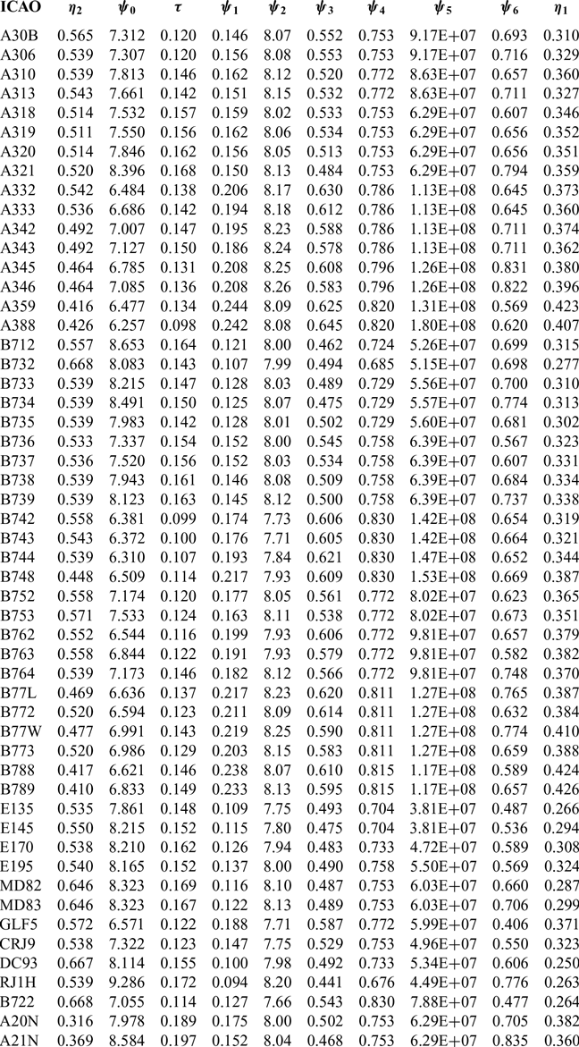
Figure 1. A comparison between the zero-lift drag coefficient (Cd ₀) estimates from Equations (7) and (23) and the high-speed, flight-test values from Obert^{(Reference Obert13)}. Solid symbols are comparisons with an Obert data point. Open symbols indicate a comparison with an estimated ‘Obert’ value based upon the aircraft total wetted area. The dashed lines indicate a ±10% variation.

5.0 THE ESTIMATION OF THE LIFT-DEPENDENT DRAG COEFFICIENT

The low-speed, lift-dependent drag coefficient appearing in Equation (4) can be broken down into four elements,

(24) \begin{equation}\left( {{1 \over {\pi{\kern-2pt}.AR.{e_{LS}}}}} \right) = \left( {{1 \over {\pi{\kern-2pt}.AR}}} \right) + \left( {{{{\delta _1}} \over {\pi{\kern-2pt}.AR}}} \right) + \left( {{{{\delta _2}} \over {\pi{\kern-2pt}.AR}}} \right) + {k_1}\end{equation}

The first is the incompressible induced, or vortex, drag for an isolated wing having the same aspect ratio as the reference wing and an elliptic spanwise load distribution; see, for example, Shevell^{(Reference Shevell4)} (chapter 9). This is the absolute minimum drag that the configuration can have. However, in practice, wing designs never quite achieve an elliptic load distribution and the second term, δ ₁, captures the additional drag resulting from deviations from the ideal due to the effects of Mach number, taper ratio and sweep, plus those of the spanwise variations in camber and twist. This term can be determined to a high level of accuracy by standard theoretical methods, e.g. ESDU⁽¹⁶⁾ or Computational Fluid Dynamics (CFD). However, despite the dependence upon a great many variables, for a civil transport aircraft its value is found to be very small compared with unity. References (Reference Shevell4) and (9) to (Reference Obert13) suggest that typical values of δ ₁ lie in the range 0.01 to 0.05, with a reasonable average being about 0.03.

When a wing is combined with a fuselage, there is mutual interference between the two components. The fuselage generates some lift and the wing experiences both additional downwash and an increase in streamwise velocity, both of which vary across the span. The net result is that the induced drag of the wing is increased by an amount that depends, principally, upon the ratio of the fuselage diameter, b _f, to the wingspan and this is captured by the coefficient δ ₂. For a more detailed discussion of this effect see, for example, McLean^{(Reference McLean17)}and Shevell^{(Reference Shevell4)}. Using unpublished data, believed to be from the Douglas Aircraft Company, Shevell^{(Reference Shevell4)} gives a graph of δ ₂ versus b _f/s (figure 11.7). This graph suggests that this small effect is well represented by the relation

(25) \begin{equation}{\delta _2} \approx 2{\left( {{{{b_f}} \over s}} \right)^2}\end{equation}

Finally, k ₁ accounts for additional vortex drag due to any aerodynamic loading on the tailplane and all the non-vortex, lift-dependent drag of the wing, fuselage and tailplane. This factor also depends upon many variables, including the location of the aircraft’s centre of gravity. However, it is determined, primarily, by the lift-dependent form drag of the wing. Therefore, whilst, in principle, it can be obtained from theory, or CFD, arguably, this quantity is best obtained from either flight-test data, or from empirical relations derived from flight-test data.

In Ref. Reference Obert13 (figure 40.36), Obert provides a flight-test dataset that is consistent with, and applicable to, the same flight conditions as the ‘high-speed’ subsonic Cd _o values given in his figure 40.17. Obert gives the induced drag factor for 12 of the aircraft listed in Table 1 as a function of aspect ratio and, by taking δ ₁ to be 0.03 and δ ₂ to be given by Equation (25), these data can be used to provide estimates for k ₁. Moreover, in cases where derivative aircraft are based upon the same wing design, or one with only minor modifications, e.g. the Airbus A318 to A321 family, the basic values can be attributed, without modification, to more of the aircraft in Table 1.

When no empirical data are available, an estimation relation is needed. Such relations have been proposed, e.g. by Shevell^{(Reference Shevell4)} (figure 11.8), and, as noted by Poll and Schumann^{(Reference Poll and Schumann2)}, Shevell’s values are well represented by the relation

(26) \begin{equation}{k_1} \approx 0.80\left( {1 - 0.53cos\left( {{\varLambda _w}} \right)} \right){\left( {C{d_o}} \right)_{M=0.5}},\end{equation}

where Λ _w is the wing’s quarter-chord sweep angle. Shevell does not give any indication of accuracy. However, whilst Obert’s results exhibit large type-to-type variation, with k ₁ ranging from 0.004 to 0.012, a ‘least squares’ fit suggests that Obert’s values follow the general trend proposed by Shevell, but with slightly different values for the coefficients, i.e.

(27) \begin{equation}{k_1} \approx 0.83\left( {1 - 0.55cos\left( {{\varLambda _w}} \right)} \right){\left( {C{d_o}} \right)_{M=0.5}}\end{equation}

This relation is subject to a maximum spread of about ±50%. However, for the range of sweep angles of practical interest, i.e. 0–40°, Equations (26) and (27) differ by less than 1%. This is taken as confirmation that Equation (26) is valid. The large uncertainty swamps any small variations in Cd _o due to changes in Reynolds number.

Estimates for the low-speed Oswald factor, e_LS, have been obtained from Equation (24), taking δ ₁ to be 0.03, δ ₂ from Equation (25) and k ₁ from Equation (26). These have then been used to generate the lift-dependent, drag coefficient for each aircraft. A comparison between the present values and either Obert’s data points, where possible, or estimates generated from Obert’s own mean line through his data is given in Fig. 2. Obert assumes that k ₁ has a constant value of 0.007, with the sum of δ ₁ and δ ₂ being 0.05. However, since the deviations are less than ±8%, it may be concluded that e _LS is not particularly sensitive to the large uncertainties implicit in the estimate of k ₁.

Figure 2. A comparison between the estimated lift-dependent drag coefficient and flight test values from the Obert^{(Reference Obert13)}. Test conditions are described as ‘average centre of gravity position’ and ‘Mach numbers greater than 0.4’ but with no ‘compressibility effects’. Solid symbols are comparisons with actual Obert values. Open symbols indicate a comparison with values from Obert’s mean line based upon aspect ratio. The dashed lines indicate a ±8% variation.

Therefore, there are two ways to approach the problem of estimating the low-speed Oswald factor. The first is to use the values of k ₁ derived from Obert’s figure 40.36 for those aircraft to which they apply and to their derivative types. However, the absolute accuracy of the Obert values is not known. The alternative is to use Equation (26) in all cases. However, this equation is known to have a maximum uncertainty of about ±50%. At this stage in the development of the method, Equation (26) has been used for all the aircraft. Further work is required if this uncertainty is to be reduced.

Finally, many modern aircraft have wing tip devices to reduce cruise drag and some designs can be retrofitted to older aircraft. Whilst the detailed characteristics of these devices vary considerably and a full analysis of their aerodynamic effects is a complex task, their overall effect is to increase the value of the Oswald factor. According to Torenbeek^{(Reference Torenbeek12)}, practical devices increase the Oswald factor by between 5% and 10%. Therefore, noting the basic level of uncertainty in the estimation method and in the interests of simplicity, if an aircraft has wing tip devices of any kind, the Oswald factor, based upon the wing without the devices fitted, should be increased by 7.5%.

6.0 THE ESTIMATION OF THE WAVE-DRAG COEFFICIENT

As the flight Mach number increases from an initial low value, sonic conditions will eventually be reached at the point on the aerofoil surface where the local static pressure has its lowest value. Usually, this lies close to the leading edge on the wing’s upper surface. Further increases in speed result in the formation of a region of supersonic flow that is bounded by the wing surface, a ‘sonic interface’Footnote ³ and, if the Mach number is sufficiently high, a terminating shockwave. Once such a ‘supersonic zone’ is established, when either M _∞ or C _Lis increased, the aircraft drag rises and the terminating shockwave moves rearwards. Whilst this zone is confined to the front portion of the wing, the drag increases are modest, being typically less than 10 drag countsFootnote ⁴, and the variation is known as ‘drag creep’. However, when the terminating shockwave moves onto the rear part of the wing, the rate of drag rise with increasing Mach number, or increasing C _L, becomes very large and this is usually referred to as ‘drag rise’. Since both the creep and rise regimes are linked to the formation and subsequent development of shockwaves, the resulting drag increments are collectively known as ‘wave’ drag.

Wave drag is a complex phenomenon. However, Shevell^{(Reference Shevell4,Reference Shevell and Bayan18)} has developed an approximate method, albeit in fragmented form, for the estimation of wave drag in two-dimensional flow as a function of lift coefficient and the wing thickness-to-chord ratio. No indication of accuracy is provided. However, once again it is highly likely that the method was developed using data from the Douglas Aircraft aerodynamics section. Curve fitting Shevell’s graphs and applying streamwise shear to extend the relations to cover the infinite-swept wingFootnote ⁵ case gives a simple, first order method for the estimation of the element of wave drag, δD _w, acting on a thin streamwise strip of wing with length c and width δy. Here, c is the streamwise wing chord and y is the spanwise distance measured along the normal to the fuselage centre line. The model suggests that the element of wave drag is a function of Mach number, wing geometry and the element of lift, δL, also acting on the strip, i.e.

(28) \begin{align}{{\delta {D_w}} \over {\left( {\gamma /2} \right){p_\infty }M_\infty ^2c\delta y}} &\approx {cos}^3\left( {{\varLambda _w}} \right)\bigg( 0.016{{\left( {{{{M_\infty }{{cos}}\left( {{\varLambda _w}} \right)} \over {{M_{ref}}}} - 0.75} \right)}^2}\nonumber \\ &\quad +6.5{{\left( {{{{M_\infty }{{cos}}\left( {{\varLambda _w}} \right)} \over {{M_{ref}}}} - 0.92} \right)}^4} \bigg),\end{align}

where

(29) \begin{equation}{M_{ref}}=0.90 - 0.10\left( {{{{C_l}} \over {{\rm{co}}{{\rm{s}}^2}({{\varLambda _w}}}}} \right) - 0.96\left( {{{t/c} \over {{\rm{cos}}( {{\varLambda _w}})}}} \right)\!,\end{equation}

t is the maximum wing thickness and the local lift coefficient, C _l, is given by

(30) \begin{equation}{C_l} = {{\delta L} \over {\left( {\gamma /2} \right){p_\infty }M_\infty ^2c\delta y}}\end{equation}

To estimate the total wave drag for a finite wing, it is necessary to know the spanwise distribution of both C _l and the thickness-to-chord ratio. However, modern civil transport wings tend to have similar spanwise variations of chord, t/c and lift; see, for example, Obert^{(Reference Obert13)} (chapter 24). Exploiting this observation, typical normalised lift distributions for sweep angles of 25° and 32° have been generated from the wing case studies presented by Obert and these are shown in Fig. 3. The effect of sweep angle is found to be small, but not insignificant.

Figure 3. The typical variation of the ratio of the local lift coefficient, C _l, to the overall lift coefficient, C _L, with spanwise location for two civil transport aircraft wings having different sweep angles (data from Obert^{(Reference Obert13)}, chapter 24).

In addition, on the inner part of the wing, where (2y/s) is less than about 0.35, the typical thickness-to-chord ratio distribution is given by

(31) \begin{equation}{t \over c} \approx 0.174 - 0.24\Big( {{{2y} \over s}} \Big),\end{equation}

whilst on the outer part of the wing ((2y/s) >0.35), t/c is constant with a value of about 0.09. Combining these approximate variations with Equations (28) to (30) allows an estimate of the distribution of the wave drag across the wing to be made. Finally, integration of the elemental wave drag acting on the strips over the span yields the wing’s total wave drag.

Whilst this is undeniably a crude estimate, in practical operations, the wave drag component is always small, being typically less than 10% of the zero-lift, profile drag component. Consequently, any errors introduced by inaccurate modelling of the wave drag will be small.

7.0 THE VARIATION OF ENGINE OVERALL PROPULSION EFFICIENCY

As discussed in detail by Poll^{(Reference Poll1)} and also by Cumpsty and Heyes^{(Reference Cumpsty and Heyes19)}, dimensional analysis can be used to show that η _o depends only upon the ratio of the total temperature at the turbine entry, (T _o)_TE, to the atmospheric freestream total temperature, (T _o)_∞ and the Mach number, whilst the precise form of the function depends upon the engine type, i.e.

(32) \begin{equation}{\eta _o} = {f_5}\left( {{{{{\left( {{T_o}} \right)}_{TE}}} \over {{{\left( {{T_o}} \right)}_\infty }}},{M_\infty }} \right)\end{equation}

The thrust coefficient, C _t, also depends upon the same parameters, i.e.

(33) \begin{equation}{C_t} = {{{F_n}} \over {\left( {\gamma /2} \right){p_\infty }M_\infty ^2{A_e}}} = {f_6}\left( {{{{{\left( {{T_o}} \right)}_{TE}}} \over {{{\left( {{T_o}} \right)}_\infty }}},{M_\infty }} \right)\!,\end{equation}

where F _n is the total net thrust generated and A _e is the sum of the engine core and bypass jet exit cross-sectional areas of all the engines. Hence,

(34) \begin{equation}{\eta _o} = {f_7}\left( {{C_t},{M_\infty }} \right)\end{equation}

The typical form of the function f ₇ is given in Fig. 4. These are for a turbofan engine with a bypass ratio of about 4.5 and are taken from Appendix B of Poll^{(Reference Poll1)}.

Figure 4. The variation of the engine overall efficiency,η _o, with thrust coefficient ${M_\infty }=0.9$, C _t and Mach number for a typical turbo-fan engine with a bypass ratio of about 4.5 – derived from data presented in figure 8.2 of Cumpsty and Heyes^{(Reference Cumpsty and Heyes19)}.

At fixed Mach number, η _o exhibits a maximum at a particular value of the thrust coefficient. Consequently, in the vicinity of the maximum, η _o is only weakly dependent upon C _t. The loci of these maximum values follow the dashed line and the variation of the maximum η _owith Mach number may be represented, to a good approximation, by the relation

(35) \begin{equation}{\left( {{\eta _o}} \right)_B} = {\eta _1}{\left( {{M_\infty }} \right)^{{\eta _2}}}\end{equation}

The coefficients η ₁ and η ₂ depend only upon the engine type and for the engine given in Fig. 4, the values are 0.36 and 0.65, respectively. This expression can be extended to a more general form by noting that η ₂ depends primarily on the engine’s nominalFootnote ⁶ bypass ratio, BPR. This is demonstrated in ESDU⁽²⁰⁾, section B3.2, figure B1, where real, though anonymised, engine data are used to show the approximate form of the relationship. Based upon these data, the expression

(36) \begin{equation}{\eta _2} = {{{M_\infty }} \over {{{\left( {{\eta _o}} \right)}_B}}}{{d{{\left( {{\eta _o}} \right)}_B}} \over {d{M_\infty }}} \approx 0.70\left( {1 - 0.045\left( {BPR} \right)} \right)\end{equation}

is believed to be accurate to ±15%. Values for the nominal bypass ratio for the engines considered in this study are obtained from the ICAO engine emissions data bank⁽⁹⁾ and are listed in Table 1.

For the engine shown in Fig. 4, the variation of overall efficiency with thrust coefficient is approximately

(37) \begin{equation}{{{\eta _o}} \over {{{\left( {{\eta _o}} \right)}_B}}} \approx 1 - 0.53\left( {1 - 0.84M_\infty ^2} \right){\left( {{{{C_t}} \over {{{\left( {{C_t}} \right)}_B}}} - 1} \right)^2}+0.25{\left( {{{{C_t}} \over {{{\left( {{C_t}} \right)}_B}}} - 1} \right)^3},\end{equation}

where the (η _o)_B and (C _t)_B pairs lie on the dashed line (maximum efficiency line) given in Fig. 4. Once again, in general, the coefficients in this relation will be engine type specific. However, deviations from the values given by this expression are likely to be small.

8.0 THE EFFECT OF MACH NUMBER ON THE DRAG POLAR WHEN THE REYNOLDS NUMBER IS CONSTANT

Equations (4), (24)–(28) and (35)–(37) can be combined to give an approximate, but physically complete, model of the variation of (η _oL/D) with the overall lift coefficient and the Mach number when the Reynolds number is constant. An example calculation, based upon a typical aircraft configuration, is presented in Fig. 5. As already noted, for any given aircraft, there is a Mach number and lift coefficient pair at which (η _o.L/D)^R has its optimum value. In the example provided, this value is 5.86 and it occurs when $M_o^R$ is 0.835 and $\left( {{C_L}} \right)_o^R$ is 0.578.

Figure 5. A typical variation of (η _o L/D) with lift coefficient and Mach number at constant Reynolds number, for an aircraft with aspect ratio of 9, sweep of 32°, e _LS of 0.8 and Cd _o of 0.016. The engine characteristics are taken from Fig. 4.

At the optimum condition,

(38) \begin{equation}d{\left( {{\eta _o}L/D} \right)^R} = {{\partial {{\left( {{\eta _o}L/D} \right)}^R}} \over {\partial {{\left( {{C_L}} \right)}^R}}}d{\left( {{C_L}} \right)^R} + {{\partial {{\left( {{\eta _o}L/D} \right)}^R}} \over {\partial {M^R}}}d{M^R}=0\end{equation}

This equation is satisfied when the partial derivatives with respect to lift coefficient and Mach number are both zero.

When both the Reynolds number and the Mach number are constant, the engine efficiency is approximately constant and there is a value of lift coefficient at which the lift-to-drag ratio has a local maximum (or best) value and both quantities depend upon the Mach number. The condition is given by

(39) \begin{equation}{{\partial {{\left( {{\eta _o}L/D} \right)}^R}} \over {\partial {{\left( {{C_L}} \right)}^R}}} \approx {{{{\left( {{\eta _o}L/D} \right)}^R}} \over {{{\left( {{C_L}} \right)}^R}}}\left( {1 - {{{{\left( {{C_L}} \right)}^R}} \over {Cd}}{{\partial Cd} \over {\partial {{\left( {{C_L}} \right)}^R}}}} \right)=0\end{equation}

Hence, from Equation (4), the best value of lift-to-drag ratio is

(40) \begin{align}\left( {{L \over D}} \right)_B^R &\approx {1 \over 2}\left( {1 - {{C{d_w}} \over {C{d_0}}}\left( {1 - {1 \over 2}\left( {{{{C_L}} \over {C{d_w}}}{{\partial C{d_w}} \over {\partial {C_L}}}} \right)} \right)} \right) \nonumber\\ &\quad\times {\left( {1 + {{C{d_w}} \over {C{d_0}}}\left( {1 - {{{C_L}} \over {C{d_w}}}{{\partial C{d_w}} \over {\partial {C_L}}}} \right)} \right)^{1/2}}{\left( {{{\pi{\kern-2pt}.AR.{e_{LS}}} \over {C{d_o}}}} \right)^{1/2}}\end{align}

and it occurs when

(41) \begin{equation}\left( {{C_L}} \right)_B^R \approx {\left( {1 + {{C{d_w}} \over {C{d_0}}}\left( {1 - {{{C_L}} \over {C{d_w}}}{{\partial C{d_w}} \over {\partial {C_L}}}} \right)} \right)^{1/2}}{\left( {\pi{\kern-2pt}.AR.{e_{LS}}C{d_0}} \right)^{1/2}}\end{equation}

Therefore, the best (η _o.L/D)^R at a given Mach number is approximately equal to the product of η _o, from Equation (35) and the corresponding best (L/D)^R from Equation (40).

The value of the Mach number at which the optimum condition occurs comes from a solution of

(42) \begin{equation}{{\partial {{\left( {{\eta _o}L/D} \right)}^R}} \over {\partial {M^R}}} = {{{{\left( {{\eta _o}L/D} \right)}^R}} \over {{M^R}}}\left( {{{{M^R}} \over {{\eta _o}}}{{d{\eta _o}} \over {d{M^R}}} - {{{M^R}} \over {Cd}}{{\partial Cd} \over {\partial {M^R}}}} \right)=0,\end{equation}

i.e. when there is a balance between the rate of wave drag rise with increasing Mach number, driving (L/D) down, and the rate of engine overall efficiency increase with increasing Mach number, driving η _o up. This is achieved when

(43) \begin{equation}{{{M^R}} \over {Cd}}{{\partial C{d_w}} \over {\partial {M^R}}} = {\eta _2}\end{equation}

Therefore, from Equation (36), in addition to the aspect ratio, sweep angle, e _LS and Cd _o, the engine bypass ratio, BPR, is also a factor determining the optimum condition.

Continuing with the example, the variation of Cd with C _L² when the Mach number has the optimum value is shown in Fig. 6. Despite the complexity of the calculation, Cd still exhibits an almost linear variation with C _L² and a ‘least-squares’ fit gives

(44) \begin{equation}Cd \approx 0.0159+0.0470C_L^2\end{equation}

Figure 6. A comparison between the high-speed drag polar at the Mach number for optimum (η _oL/D)^R and low-speed drag polar for the aircraft used in Fig. 5.

However, in the absence of wave drag, the polar Equation (4) is

(45) \begin{equation}Cd = {\left( {C{d_0}} \right)_{M=0.5}} + \left( {{1 \over {\pi{\kern-2pt}.AR.{e_{LS}}}}} \right)C_L^2=0.0160+0.0437C_L^2\end{equation}

Therefore, when the lift coefficient is also at its optimum value (C _L = 0.578), relative to Equation (45), Cd has risen by 10 drag counts (≈3.3% increase) and the gradient of the polar has grown by about 0.0033 (≈7.5% increase). However, the values of Cd ₀ are almost the same. This suggests that the zero-lift, profile drag coefficient is essentially unchanged by the development of wave drag (<1%). This insensitivity, whilst perhaps surprising, is consistent with the assumption made in Equation (4) and with the Obert data given in Fig. 1. Therefore, according to the Shevell model, the principal effect of wave drag at the conditions for optimum (η _oL/D)^R is to decrease the value of the Oswald factor relative to its low-speed value.

When the Mach number is equal to $M_o^R$, Equation (4) becomes

(46) \begin{equation}Cd \approx C{d_0} + \left( {{{{e_{LS}}} \over {{e_o}}}} \right)\left( {{1 \over {\pi{\kern-2pt}.AR.{e_{LS}}}}} \right)C_L^2\end{equation}

Using this relation in Equation (39) to obtain (L/D)_o and also using Equation (35) gives

(47) \begin{equation}\left( {{\eta _o}L/D} \right)_o^R \approx {{\left( {{\eta _o}} \right)_o^R} \over 2}{\left( {\pi{\kern-2pt}.AR.{e_{LS}}\left( {{{{e_o}} \over {{e_{LS}}}}} \right)} \right)^{1/2}}{\left( {{1 \over {C{d_0}}}} \right)^{1/2}},\end{equation}

(48) \begin{equation}\left( {{L \over D}} \right)_o^R \approx {1 \over 2}{\left( {\pi{\kern-2pt}.AR.{e_{LS}}\left( {{{{e_o}} \over {{e_{LS}}}}} \right)} \right)^{1/2}}{\left( {{1 \over {C{d_0}}}} \right)^{1/2}}\end{equation}

and

(49) \begin{equation}\left( {{C_L}} \right)_o^R \approx {\left( {\pi{\kern-2pt}.AR.{e_{LS}}.\left( {{{{e_o}} \over {{e_{LS}}}}} \right)} \right)^{1/2}}C{d_0}^{1/2}\end{equation}

For consistency between Equations (40) and (41) and (48) and (49), at the optimum condition,

(50)\begin{equation}\left( {{{{C_L}} \over {C{d_w}}}{{dC{d_w}} \over {d{C_L}}}} \right)_o^R=2\end{equation}

and, hence, from Equations (41) and (49)

(51) \begin{equation}{{{e_o}} \over {{e_{LS}}}} \approx 1 - \left( {{{C{d_w}} \over {C{d_0}}}} \right)_o^R\end{equation}

Whilst this is a very simple result, it is a consequence of the definition of ‘wave drag’ as used in the Shevell model, i.e. according to Equations (4), and Equation (51) may not hold if the wave drag is defined in a different way.

Calculations have been carried out for the two loading distributions shown in Fig. 3 for aircraft with aspect ratios in the range of 7.5–10 and Cd _o lying between 0.014 and 0.02. The results show that, when the Mach number is at $M_o^R$, Cd ₀ varies by a maximum of 2%. In addition, the increase in the lift-dependent drag coefficient due to wave drag is given, to an accuracy of ±10%, by the expression

(52) \begin{equation}\left( {{{dC{d_w}} \over {dC_L^2}}} \right)_o^R = {{{\delta _3}} \over {\pi{\kern-2pt}.AR}} \approx 0.167\left( {{\eta _2}{e_{LS}}} \right)\end{equation}

Hence, the total lift-dependent drag coefficient may be written as

(53) \begin{equation}\left( {{1 \over {\pi{\kern-2pt}.AR.{e_o}}}} \right) \approx \left( {\left( {{{1 + {\delta _1} + {\delta _2} + {\delta _3}} \over {\pi{\kern-2pt}.AR}}} \right) + {k_1}} \right)\end{equation}

Taking typical values, the contributions of the various elements to the total lift-dependent drag coefficient are approximately 80% from the wing vortex system, 15% from the profile and trim drags and 5% from the wave drag. Since the contribution from wave drag is so small, a relatively crude estimate does not introduce any significant inaccuracy into the overall estimation process. Therefore, using more sophisticated methods to determine wave drag, e.g. CFD, would greatly increase the complexity of the calculation, but would have little impact upon the result. The largest uncertainty in the estimate is still that associated with the value of k ₁.

Furthermore, curve fitting the data suggests that the relation

(54) \begin{equation}{{{e_o}} \over {{e_{LS}}}} \approx 0.992 - 0.11({{\eta _2}{e_{LS}}})\end{equation}

is accurate to ±0.5%. This relation is shown in Fig. 7.

Figure 7. The variation of the ratio of the high-speed and low-speed Oswald factors, e _o/e _LS, with the product of η₂ and the low-speed Oswald factor, e _LS.

Finally, by combining Equations (51) and (54), the wave drag coefficient at the optimum condition is

(55) \begin{equation}\left( {C{d_w}} \right)_o^R \approx 0.11({{\eta _2}{e_{LS}}})C{d_0},\end{equation}

whilst, to within ±2%, the total drag coefficient is given by

(56) \begin{equation}\left( {Cd} \right)_o^R \approx 1.99C{d_0}\end{equation}

The calculations also show that the Mach number at which the optimum occurs, $M_o^R$, exhibits a very weak dependence upon Cd ₀. This is consistent with the assumption made in Ref. Reference Poll and Schumann2 that $M_o^R$ is independent of Cd ₀ and, hence, Reynolds number. However, $M_o^R$ does have some dependence on η₂, i.e.

(57) \begin{equation}{{\partial M_o^R} \over {\partial {\eta _2}}} \approx 0.06\end{equation}

Therefore, if an aircraft’s engines are replaced with ones having a different bypass ratio, the optimum Mach number for the new combination will be slightly different.

9.0 THE CHARACTERISTIC PARAMETERS

It is now possible to write down expressions for all the ψ parameters. As already shown, ψ₀comes from Equation (23) and depends only upon aircraft geometry. In principle, ψ₁ can be obtained from Equation (47). However, since there is no simple, accurate method available for the estimation of η _o, at this stage in the development of the method Ψ ₁ is best obtained from empirical data. This process is described in detail in the next section.

The value of τ comes from Equations (8), (23)–(26) and (54), i.e.

(58) \begin{equation}\tau = - \left( {{{C_F^{ac}} \over {{e_o}}}} \right)\left( {{{d{e_o}} \over {dC_F^{ac}}}} \right) \approx {{\left( {0.992 - 0.22\left( {{\eta _2}{{\left( {{e_{LS}}} \right)}_o}} \right)} \right)} \over {\left( {0.992 - 0.11\left( {{\eta _2}{{\left( {{e_{LS}}} \right)}_o}} \right)} \right)}}\left( {\pi{\kern-2pt}.AR.{k_1}.{{\left( {{e_{LS}}} \right)}_o}} \right)\end{equation}

In this analysis, τ is a constant. Therefore, in Equation (58), e _LS should be evaluated at the optimum Reynolds number for a value of the aircraft mass that is near the middle of the operating range. Sample estimates for the aircraft listed in Table 1 show that this requirement is satisfied if m/MTOM is taken to be 0.8, see Equation (16). The corresponding value of E _o is given by

(59) \begin{equation}{E_o} = \left( {0.992 - 0.11{\eta _2}{{\left( {{e_{LS}}} \right)}_o}} \right){\left( {{e_{LS}}} \right)_o}{\left( {{{\left( {C_F^{ac}} \right)}_o}} \right)^\tau }\end{equation}

The parameter ψ₂ can now be determined by combining Equations (8), (10), (23) and (49), i.e.

(60)\begin{equation}{\psi _2} \approx {\left( {\pi{\kern-2pt}.AR.{\psi _0}.{E_o}} \right)^{1/2}}\end{equation}

Similarly, $\psi $₃ comes from Equations (8), (11), (23) and (48), i.e.

(61) \begin{equation}{\psi _3} \approx {1 \over 2}{\left( {{{\pi{\kern-2pt}.AR.{E_o}} \over {{\psi _0}}}} \right)^{1/2}}\end{equation}

As shown in Poll^{(Reference Poll1)}, estimates of (η _oL/D) are sensitive to ψ₄ and therefore this quantity needs to be determined as accurately as possible. As indicated above, in principle, ψ₄, which is equal to $M_o^R$ – see Equation (12), can be calculated directly from the wave drag model. However, since the Shevell method is highly simplified, the absolute accuracy of such an estimate is unknown. Therefore, in the first instance, an alternative approach is required.

The most accurately known speed is the maximum operational Mach number, M _MO, since this is specified in the TCDS. In addition, the long-range cruise Mach number, M _LRC, is often to be found in either the aircraft APR, or other standard reference sources, e.g. Jane’s^{(Reference Jackson7)}. Figure 8 shows the variation of M _LRC with M _MO for those aircraft in Table 1 for which M _LRC is known. There is a strong correlation between the two quantities and taking M _LRC to be 0.935(M _MO) gives a maximum error of about 4%. This relation can then be extended to provide an estimate of the maximum range cruise Mach number, M _MRC, (= M _o) by noting that, from equation (24) of Poll^{(Reference Poll1)}, M _LRC is approximately 1.035 times M _MRC. Hence,

(62) \begin{equation}{\psi _4} = {M_o} = {M_{MRC}} \approx {{{M_{LRC}}} \over {1.035}} \approx 0.910{M_{MO}}\end{equation}

Figure 8. The relationship between the long-range cruise Mach number, M _LRC, and the maximum operational Mach number, M _MO. The solid line is given by M _LRC equal to 0.940M _MO, and the dashed lines represent ±4% variation.

To minimise the error, if the long range cruise Mach number is accurately known, ψ₄ is taken to be M _LRC divided by 1.035. However, If M _LRC is not available, then Equation (62) should be used. Estimated values of ψ₄ are given in Table 2.

The parameter ψ₅ in Equation (14) is the non-dimensional, wing reference area. Unlike the plan area of the exposed, or ‘wetted’, part of the wing, which is easily and unambiguously obtained from a general arrangement drawing, the aerodynamic reference area, S _ref, must be given a clear definition. This is because the ‘reference’ area includes part of the wing that is covered by the fuselage. In this analysis, S _ref is defined as the plan area of the exposed wing plus the area of the rectangle inside the fuselage whose vertices are the points where the leading and trailing edges meet the fuselage sideFootnote ⁷. The values of S _ref are listed in Table 1, and the corresponding values of ψ₅ are given in Table 2.

Finally, the parameter ψ₆ in Equation (15) is the non-dimensional, maximum take-off mass. However, whilst a given aircraft type will have a fixed external geometry and specified engines, its MTOM is not necessarily fixed. This is because the manufacturer usually offers a number of ‘weight variants’ to satisfy different airline requirementsFootnote ⁸. Therefore, the MTOM may have a range of values, with the largest being as much as 25% greater than the smallest. For a particular aircraft, the weight variant can usually be found from the tail number. Table 1 contains a reference MTOM and the corresponding weight variant number for each aircraft, and the corresponding values of (ψ₆)_ref are given in Table 2. The reference value can be converted to cover other aircraft by introducing a weight variant factor, F _wv, i.e.

(63) \begin{equation}{\psi _6} = {F_{wv}}{\left( {{\psi _6}} \right)_{ref}},\end{equation}

where F _wv is the ratio of the actual MTOM, as given either in the type certificate, or the relevant APR, to the MTOM of the reference aircraft.

10.0 THE ESTIMATION OF Ψ ₁ FROM THE PAYLOAD–RANGE DIAGRAM

APRs usually contain a number of payload–range diagrams whose construction requires a knowledge of (η _oL/D). Consequently, with suitable interpretation, these diagrams can be used to provide estimates of (η _oL/D)_o under specified conditions and, hence, values of Ψ ₁can be established.

At the beginning of the take-off run (brakes-off point), the take-off mass, TOM, can be broken down into a number of components, i.e.

(64) \begin{equation}TOM = OEM + PM + F{M_{nc}} + TFM = ZFM + F{M_{nc}} + TFM\end{equation}

Here PM is the payload mass, TFM is the mass of the fuel that will be used during the trip, FM _nc is the mass of the fuel that is not consumed during the flight and OEM is the operational empty mass. The OEM is the mass of the aircraft before any payload and fuel are loaded and is given by

(65) \begin{equation}OEM = MZFM - MPM,\end{equation}

where MZFM is the maximum permitted zero-fuel mass (given in the aircraft type certificate) and MPM is the maximum payload. The MZFM and typical values of the MPM are usually given in the aircraft’s APR.

As described by Poll^{(Reference Poll1)}, the trip fuel mass is related to the take-off mass by

(66) \begin{equation}{{TFM} \over {TOM}} = {\alpha _t} \approx 1 - EXP\left( { - \left( {{X_t} + {\varepsilon _t}} \right)} \right)\!,\end{equation}

where X _t is the non-dimensional trip distance, given by

(67) \begin{equation}{X_t} = {{g{R_t}} \over {{{\left( {{\eta _o}L/D} \right)}_o}LCV}},\end{equation}

with R _tbeing the great circle distance between the departure and destination points, ε _t the total ‘lost fuel’ index and LCV the lower calorific value of the fuel. The total lost fuel index captures the additional fuel used in the climb and descent phases, any fuel wasted by not cruising at the optimum speed and height, any fuel used to fly extra distance due to route deviations and fuel lost, or saved, because of the wind. However, for a maximum range cruise in still air

(68) \begin{equation}{\varepsilon _t} = {\left( {{\varepsilon _{cd}}} \right)_{min}} + \left( {{{1 - n} \over n}} \right){X_t},\end{equation}

where ε _cd is the sum of the lost fuel indices for the climb and descent phases and n is given by

(69) \begin{equation}n = {{{{\left( {{\eta _o}L/D} \right)}_{avg}}} \over {{{\left( {{\eta _o}L/D} \right)}_o}}}\end{equation}

In general, the parameter n depends upon the flight trajectory, i.e. the profile of Mach number versus altitude, and the aircraft’s mass at the beginning of the cruise.

The non-consumed fuel, some of which may be used on subsequent flights, must be greater than, or equal to, the minimum reserve fuel, FM _res, as required by the regulatory authority, plus any extra fuel, FM _ext, specified by the operator, or the aircraft captain. However, for a maximum range flight with a given amount of trip fuel, the non-consumed fuel must also have its minimum possible value and so

(70) \begin{equation}{\left( {F{M_{nc}}} \right)_{min}} = {\left( {F{M_{res}}} \right)_{min}} = {\beta _{min}}TOM\end{equation}

Hence, from Equations (64), (66) and (70),

(71) \begin{equation}{\alpha _t}=1 - {\beta _{min}} - {{ZFM} \over {TOM}}\end{equation}

and, on the payload–range diagram, the variation of zero-fuel mass with range for a given take-off mass is given by

(72) \begin{equation}{{ZFM} \over {TOM}} = EXP\left( { - \left( {{{\left( {{\varepsilon _{cd}}} \right)}_{min}} + {{{X_t}} \over n}} \right)} \right) - {\beta _{min}}\end{equation}

In Appendix C, it is shown that, under EU Ops rules (see Airbus⁽²³⁾), the reserve fuel requirement can always be expressed in the form

(73) \begin{equation}{\beta _{min}} \approx 0.05{\alpha _t} + \lambda \left( {1 - {\alpha _t}} \right) = {{\left( {0.05 + \left( {\lambda - 0.05} \right)\left( {ZFM/TOM} \right)} \right)} \over {\left( {1.05 - \lambda } \right)}},\end{equation}

where

(74) \begin{equation}\lambda = \left( {{{\left( {{\varepsilon _{cd}}} \right)}_{min}} + {{\left( {{X_{ad}} + {X_{da}} + {X_{fr}}} \right)} \over n}} \right)\end{equation}

Here, X _ad, X _da and X _fr are the non-dimensional, additional cruise distances that can be flown using the ‘additional’, ‘diversionary airport’ and ‘final reserve’ elements of the reserve fuel. Combining Equations (72) and (73) gives

(75) \begin{equation}{{ZFM} \over {TOM}} = \left( {{{1.05 - \lambda } \over {EXP{{\left( {{\varepsilon _{cd}}} \right)}_{min}}}}} \right)EXP\left( { - {{{X_t}} \over n}} \right) - 0.05\end{equation}

This equation is the tool that is used to extract data from the payload range diagram and, to check the accuracy of the results, two implementation techniques have been used.

10.1 Method 1

On the payload–range diagram, each point represents a complete flight. If the aircraft is always operating at optimum (η _oL/D), the appropriate cruise altitude and, hence, the Reynolds number is determined by the aircraft mass, m – see Equation (20). This being the case, (η _oL/D)_o also varies with m – see Equation (21). The value of (η _oL/D)_o at the beginning of the cruise is determined, primarily, by the take-off mass and, as the aircraft consumes fuel, both m and (η _oL/D)_o decrease. However, since the variation is usually small, to a good approximation, a complete flight may be characterised by the average value of the mass in cruise.

As noted in Ref. Reference Poll1, at the start of cruise, the mass is about 97.5% of TOM and, at the end, it is roughly 101% of the landing mass, LM Footnote ⁹. Therefore, using Equations (66)–(68) and taking (ε _cd)_min to be 0.0067 – see Poll^{(Reference Poll1)},

(76) \begin{equation}{{{m_{avg}}} \over {TOM}} = {{\left( {{m_{ic}} + {m_{fc}}} \right)} \over {2({TOM})}} \approx {1 \over 2}\left( {1.985 - 1.01{{TFM} \over {TOM}}} \right) \approx 0.99\left( {1.0 - 0.51{{{X_t}} \over n}} \right)\end{equation}

and, from Equations (21), (67) and (69), for flight in the International Standard Atmosphere,

(77) \begin{equation}{{{X_t}} \over n} = {{g{R_t}} \over {\left( {n{\psi _1}} \right)LCV}}{\left( {\left( {{a \over {\psi _5^b}}} \right){{\left( {{\psi _7}\Big( {{{MTOM} \over {TOM}}} \Big)\left( {{{TOM} \over {{m_{avg}}}}} \right)} \right)}^{b{\iota _o}{\kappa _o}}}} \right)^{\left( {{{1 + \tau } \over 2}} \right)}}\end{equation}

Substituting the results from Equation (76) into Equation (77), neglecting terms that are small in comparison with unity and rearranging gives

(78) \begin{equation}{{{X_t}} \over n} \approx \left( {{{{\psi _8}g{R_t}} \over {n{\psi _1}LCV}}} \right)\left( {1+0.51\left( {b{\iota _o}{\kappa _o}} \right)\left( {{{1 + \tau } \over 2}} \right)\left( {{{{\psi _8}g{R_t}} \over {n{\psi _1}LCV}}} \right)} \right)\!,\end{equation}

where

(79) \begin{equation}{\psi _8} = {1 \over {{G_5}}}{\left( {\left( {{a \over {\psi _5^b}}} \right){{\left( {{{{\psi _7}} \over {0.99}}\Bigg( {{{MTOM} \over {TOM}}} \Bigg)} \right)}^{b{\iota _o}{\kappa _o}}}} \right)^{\left( {{{1 + \tau } \over 2}} \right)}}\end{equation}

Hence, by substituting the result from Equation (78) into Equation (75) and expanding the exponential function as a power series gives

(80) \begin{align}{{ZFM} \over {TOM}}+0.05 &= \left( {{{1.05 - \lambda } \over {EXP\left( {{{\left( {{\varepsilon _{cd}}} \right)}_{min}}} \right)}}} \right)\left( {1 - \left( {{{{\psi _8}g{R_t}} \over {n{\psi _1}LCV}}} \right) } \right. \nonumber\\ &\quad+ \left. {{1 \over 2}\left( {1 - 1.01\left( {b{\iota _o}{\kappa _o}} \right)\Bigg( {{{1 + \tau } \over 2}} \Bigg)} \right){{\left( {{{{\psi _8}g{R_t}} \over {n{\psi _1}LCV}}} \right)}^2} - \ldots } \right)\end{align}

For a given aircraft, (ε _cd)_min is fixed and, as argued in Ref. Reference Poll1, its value is expected to be approximately 0.0067 ± 0.0026. Therefore, for any particular value of TOM, if the reserve fuel coefficient, $\lambda$, the distance flown, R _t, ψ₈ and the zero-fuel mass, ZFM, are known, the value of (nΨ ₁) can be deduced. However, whilst R _t and ZFM may be read directly from the payload–range diagram, $\lambda$ is usually not known ‘a priori’. Consequently, a calculation scheme is required to determine the combined values of (nΨ ₁) and τ that best describe the given variation of ZFM with R _t at fixed TOM.

To test the robustness of the results, two independent numerical schemes have been used. Method 1 involved the inversion of Equation (80) and, with $\lambda$ fixed, using known values of ZFM and R _t taken along a line of constant TOM to determine (nΨ ₁) directly. The value of $\lambda$ was then varied until the ‘least squares’ linear fit of (nΨ ₁) against R _t had a zero slope, i.e. both (nΨ ₁) and $\lambda$ had single values for the whole dataset. An example showing the success of the fitting process is given in Fig. 9.

Figure 9. The payload–range diagram for the Boeing 777-300ER. Lines of constant take-off mass are constructed using the estimates, based upon method 1, for (nΨ ₁) and $\lambda$ and the circles are the digitised values taken from the manufacture’s payload–range diagram. The values of (nΨ ₁) and are 0.320 ± 0.001 and 0.030 ± 0.003 respectively.

It was found that each payload–range diagram only yielded a single value of (nΨ ₁) and the variations in the values of both (nΨ ₁) and for different values of TOM/MTOM were generally small. The values of (nΨ ₁) were not sensitive to the choice of (ε _cd)_min. However, when the range parameter was small, (nΨ ₁) was found to be very sensitive to errors in ZFM/TOM. These observations are all consistent with the behaviour implicit in Equation (80). The accuracy demonstrated in Fig. 9 was not achieved in all cases. However, the larger discrepancies were found to be due, primarily, to inaccuracies and inconsistencies in the payload–range diagrams given in some APRs.

10.2 Method 2

For method 2, it was assumed that the Reynolds number effects were small and, using the same values of ZFM versus Rt at fixed TOM, Equation (75) was solved numerically to determine pairs of values of (η _oL/D)_avg and $\lambda$ for which the data fit had the minimum least square root of the sum of deviations (Appendix D). The values of (η _oL/D)_avg were then converted to (nΨ ₁) by using Equations (21) and (67), with the mid-range value being taken for R _t. The results from the two methods for all the aircraft considered in this study are compared in Fig. 10. The values obtained from the two methods were found to have a maximum difference of 5% and a mean difference of 1.5%. The ‘best estimate’ for (nΨ ₁) was taken to be the average of the two values.

Figure 10. A comparison between the values of (nΨ ₁) as determined by analysis methods 1 and 2. The solid line has unit slope and the dashed lines indicate a ±5% variation.

The (η _oL/D)_avg values obtained by method 2 can also be compared directly with those given in other references, e.g. Martinez-Val et al.^{(Reference Martinez-Val, Palacin and Perez21)} and Randle et al.^{(Reference Randle, Hall and Vera-Morales22)}. In both of those studies, the authors sought to estimate (η _oL/D)_avg either from payload–range diagrams or from flight data recorder information, and results are provided for 20 of the aircraft listed in Table 1. These are compared with the method 2 values in Fig. 11. The Martinez-Val et al. results exhibit greater scatter than those of Randle et al. and, whilst some of this is attributable to reading errors due to the small size of the figures in both references, the general level of agreement is reasonable and reflects the sensitivity of the estimates to small errors in the input data.

Figure 11. A comparison between the estimated values of (η _oL/D)_avg and the previously published results of Martinez-Val et al.^{(Reference Martinez-Val, Palacin and Perez21)} and Randle et al.^{(Reference Randle, Hall and Vera-Morales22)}. The solid line has unit slope, and the dashed lines indicate a ±10% variation.

Finally, to obtain Ψ ₁, it is necessary to estimate the value of n; see Equation (69). This quantity may be expressed as

(81) \begin{equation}n = \left( {{{{{\left( {{\eta _o}L/D} \right)}_{IC}}} \over {{{\left( {{\eta _o}L/D} \right)}_o}}}} \right)\left( {{{{{\left( {{\eta _o}L/D} \right)}_{avg}}} \over {{{\left( {{\eta _o}L/D} \right)}_{IC}}}}} \right)\!,\end{equation}

where all the terms are evaluated at the same Reynolds number. The first bracketed term is given by Equation (22) and depends upon M _∞/M _o and the ratio of the lift coefficient at the beginning of cruise, (C _L)_IC, to the optimum value, (C _L)_o. Payload–range diagrams are usually based on a fixed take-off mass, a fixed Mach number and either a fixed altitude or a step-climb profile. In all the cases considered in this analysis, the diagram was based upon the long-range cruise Mach number. Therefore, by definition, at the start of the cruise

(82) \begin{equation}{{{{\left( {{\eta _o}L/D} \right)}_{IC}}} \over {{{\left( {{\eta _o}L/D} \right)}_o}}} \approx 0.99\end{equation}

If the aircraft were then to follow a cruise–climb trajectory, the ratio of (η _oL/D) to its optimum value would stay at this value. However, at present, to guarantee safe separation, aircraft are not allowed to cruise climb, although, if circumstances permit, an occasional step change to a higher cruise altitude may be possible. Therefore, the second bracketed term provides a further correction to allow for the additional fuel required when following constant-altitude or step-climb trajectories. As shown in Ref. Reference Poll1, if the flight trajectory is known, this term can be evaluated exactly. However, examination of the complete solution suggests that, in current operating conditions, this term is likely to have a value in the region of 0.985. Hence,

(83) \begin{equation}n \approx 0.975\end{equation}

With the value of n determined, Ψ ₁ can be estimated and the values are listed in Table 2.

11.0 THE ESTIMATION OF η _o, (L/D) AND TOTAL THRUST

From Equations (12) and (35),

(84) \begin{equation}{{\left( {{\eta _o}} \right)_B^R} \over {\left( {{\eta _o}} \right)_o^R}} = {\left( {{{{M_\infty }} \over {{\psi _4}}}} \right)^{{\eta _2}}}.\end{equation}

Since η _o depends only upon Mach number, this result can be combined with the function f ₁ from Equations (A-14), or (A-15) to give

(85) \begin{equation}{{\left( {L/D} \right)_B^R} \over {\left( {L/D} \right)_o^R}} = {{\left( {{\eta _o}L/D} \right)_B^R} \over {\left( {{\eta _o}L/D} \right)_o^R}}\left( {{{\left( {{\eta _o}} \right)_o^R} \over {\left( {{\eta _o}} \right)_B^R}}} \right) = {f_1}{\left( {{{{\psi _4}} \over {{M_\infty }}}} \right)^{{\eta _2}}}\end{equation}

Hence, at the optimum condition, using Equations (11), (17) and (19) and ignoring products of small quantities,

(86) \begin{equation}{\left( {L/D} \right)_o} \approx {G_7}{\psi _3}{\left( {\left( {{{\psi _5^b} \over a}} \right){{\left( {{1 \over {{\psi _7}}}\left( {{m \over {MTOM}}} \right)} \right)}^{b{\iota _o}{\kappa _o}}}} \right)^{\left( {{{1 + \tau } \over 2}} \right)}},\end{equation}

where

(87) \begin{equation}{G_7} = {\left(\,{{f_1}} \right)_o}{\left( {{1 \over {1 + \varepsilon }}} \right)^{{\eta _2}}}{\left( {{1 \over {{G_3}}}} \right)^{\left( {{{1 + \tau } \over 2}} \right)}} = {\left( {{1 \over {1 + \varepsilon }}} \right)^{{\eta _2}}}{G_5}\end{equation}

It follows immediately from Equations (21) and (86) that

(88) \begin{equation}{\left( {{\eta _o}} \right)_o} = {{{{\left( {{\eta _o}L/D} \right)}_o}} \over {{{\left( {L/D} \right)}_o}}} = \left( {{{{\psi _1}} \over {{\psi _3}}}} \right){\left( {1 + \varepsilon } \right)^{{\eta _2}}} = \left( {{{{\psi _1}} \over {{\psi _3}}}} \right){\left( {{{{M_o}} \over {{\psi _4}}}} \right)^{{\eta _2}}}\end{equation}

Hence, from Equation (35), the engine constant η₁ is given by

(89) \begin{equation}{\eta _1} = \left( {{{{\psi _1}} \over {{\psi _3}}}} \right){\left( {{1 \over {{\psi _4}}}} \right)^{{\eta _2}}}\end{equation}

The values of η₁are included in Table 2.

As shown in Poll^{(Reference Poll1)}, provided the engines are sized such that L/D and η_oboth reach maximum values at the same conditions in straight and level flight, then

(90) \begin{equation}{{{C_t}} \over {{{\left( {{C_t}} \right)}_B}}} \approx {{{C_L}} \over {{{\left( {{C_L}} \right)}_B}}}\end{equation}

and, assuming that Equation (37) is approximately the same for all engine types,

(91) \begin{equation}{{{\eta _o}} \over {{{\left( {{\eta _o}} \right)}_B}}} \approx 1 - 0.53\left( {1 - 0.84M_\infty ^2} \right){\left( {{{{C_L}} \over {{{\left( {{C_L}} \right)}_B}}} - 1} \right)^2}+0.25{\left( {{{{C_L}} \over {{{\left( {{C_L}} \right)}_B}}} - 1} \right)^3}\end{equation}

In addition, Poll and Schumann^{(Reference Poll and Schumann2)} have shown that, when the mass is fixed,

(92) \begin{equation}{{{C_L}} \over {{{\left( {{C_L}} \right)}_B}}} \approx \left( {{{{C_L}} \over {{{\left( {{C_L}} \right)}_o}}}} \right){{{{\left( {{C_L}} \right)}_o}} \over {{{\left( {{C_L}} \right)}_B}}} = {f_4}{\left( {{{{C_L}} \over {{{\left( {{C_L}} \right)}_o}}}} \right)^\upsilon },\end{equation}

where f ₄ and ν are given in Appendix A. Therefore, the overall engine efficiency for any combination of Mach number and lift coefficient within the range of validity of the basic relations set out in Appendix A, is given by

(93) \begin{align}{{{\eta _o}} \over {{{\left( {{\eta _o}} \right)}_o}}} &\approx {\left( {{{{M_\infty }} \over {{M_o}}}} \right)^{{\eta _2}}}\bigg( {1 - 0.53\left( {1 - 0.84M_\infty ^2} \right){{\left( {\left( {{f_4}{{\left( {{{{C_L}} \over {{{\left( {{C_L}} \right)}_o}}}} \right)}^\upsilon }} \right) - 1} \right)}^2}} \nonumber\\ &\quad +0.25{{\left( {\left( {{f_4}{{\left( {{{{C_L}} \over {{{\left( {{C_L}} \right)}_o}}}} \right)}^\upsilon }} \right) - 1} \right)}^3} \bigg).\end{align}

Furthermore, the combination of Equations (22), (86) and (93) allows the estimation of (L/D) for an aircraft of given mass to be determined for any combination of Mach number and lift coefficient, i.e.

(94) \begin{equation}\left( {L/D} \right) \approx {{\left( {{\eta _o}L/D} \right)} \over {{{\left( {{\eta _o}L/D} \right)}_o}}}{{{{\left( {{\eta _o}} \right)}_o}} \over {\left( {{\eta _o}} \right)}}{\left( {L/D} \right)_o}\end{equation}

In straight and level flight, the thrust is equal to the drag and the lift is equal to the aircraft weight and so the total engine thrust, F _n, is given by

(95) \begin{equation}{F_n} \approx {{mg} \over {\left( {L/D} \right)}}\end{equation}

12.0 SENSITIVITY TO UNCERTAINTY IN THE INPUT VALUES

The overall accuracy of the method may be judged by examining the sensitivity of (η _oL/D) to uncertainty in the values of (η _oL/D)_o, M _o and (C _L)_o. This can be expressed as

(96) \begin{equation}{{d( {{\eta _o}L/D})} \over {\left( {{\eta _o}L/D} \right)}} = {g_1}{{d{{\left( {{\eta _o}L/D} \right)}_o}} \over {{{\left( {{\eta _o}L/D} \right)}_o}}} + {g_2}{{d{M_o}} \over {{M_o}}} + {g_3}{{d{{\left( {{C_L}} \right)}_o}} \over {{{\left( {{C_L}} \right)}_o}}},\end{equation}

where

(97) \begin{equation}{g_1} = {{{{\left( {{\eta _o}L/D} \right)}_o}} \over {\left( {{\eta _o}L/D} \right)}}{{\partial ( {{\eta _o}L/D} )} \over {\partial {{\left( {{\eta _o}L/D} \right)}_o}}},\end{equation}

(98) \begin{equation}{g_2} = {{{M_o}} \over {\left( {{\eta _o}L/D} \right)}}{{\partial ( {{\eta _o}L/D})} \over {\partial {M_o}}}\end{equation}

and

(99) \begin{equation}{g_3} = {{{{\left( {{C_L}} \right)}_o}} \over {\left( {{\eta _o}L/D} \right)}}{{\partial ( {{\eta _o}L/D})} \over {\partial {{\left( {{C_L}} \right)}_o}}}\end{equation}

To simplify the analysis, the functions g ₁, g ₂ and g ₃ are derived using the constant Reynolds number functions developed by Poll^{(Reference Poll1)}.

For any combination of Mach number and lift coefficient, it can be seen that (η _oL/D) is always directly proportional to (η _oL/D)_o and so g ₁ is constant and equal to unity. However, g ₂ and g ₃ each vary with both M _∞/M _o and C _L/(C _L)_o and the forms of the relationships are given in Figs 12 and 13.

Figure 12. The variation of the function g ₂ with C _L/(C _L)_o and M _∞/(M)_o.

Figure 13. The variation of the function g ₃ with C _L/(C _L)_o and M _∞/(M)_o.

These graphs show that, in general, (η _oL/D) exhibits a greater sensitivity to errors in M _o than to errors in (C _L)_o and that, in the region around the optimum point, the values of g ₂ and g ₃ increase as both M/M _o and C _L/(C _L)_o increase. In practice, for reasons of fuel economy, aircraft tend to operate at Mach numbers between the optimum and the long-range cruise value, M _LRC; see, for example, Airbus⁽²³⁾, where M _LRC is approximately 3.5% greater than M _o; see Poll^{(Reference Poll1)}. Hence, for normal operating conditions, (M _∞/M _o) lies between 1 and 1.035. However, if there is a need to make up lost time, speeds up to about 1.05 times M _o may be used. In addition, all engines have an upper limit on cruise thrust and this imposes upper limits on C _L/(C _L)_o for each value of M/M _o. For a given speed and aircraft weight, the maximum thrust available determines the maximum altitude that can be reached and, under ISA conditions, this is usually about 2,000 to 3,000ft higher than the altitude for minimum fuel burn. In addition, Poll^{(Reference Poll1)} has shown that altitude is linked directly to the term C _L.M _∞² and, when the altitude is 2,000ft higher than the optimum for fuel burn, C _L.M _∞² is about 1.08 times (C _L)_o.M _o². This limiting line has been evaluated for flight in the ISA ⁽¹⁵⁾ and is included in the figuresFootnote ¹⁰.

It is clear from the figures that g ₂ only exceeds unity at ‘catch up’ speeds, whilst g ₃ never exceeds 0.7 at any condition. Therefore, the method has the potential to provide reasonable fuel burn rate estimates. In general, estimates of (η _oL/D) exhibit the highest sensitivity to errors in (η _oL/D)_o, since these quantities are directly proportional to one another. Next comes M _o, where, in general, there is some alleviation of errors, whilst (η _oL/D) exhibits least sensitivity to errors in (C _L)_o.

13.0 PARAMETER ACCURACY

Values of Ψ ₀ have been obtained from Equation (23) using the relations set out in Appendix B. Comparisons with a limited amount of flight-test data indicate that the values are accurate to about ±10%. Estimates of Ψ ₁ have been derived from payload–range diagrams contained in the manufactures’ APRs. Two independent schemes have been used and the results compared with the limited amount of data available from other sources. Provided that the payload–range diagrams are based upon reliable information, Ψ ₁is expected to be accurate to approximately ±5%. The Mach number at the optimum condition, M _o, has been linked to either the long-range cruise Mach number (M _o equal to 1.035(M _LRC)) or the M _MO (M _o equal to 0.910(M _MO)). When M _LRC is obtained from either the APR, or the FCOM, the resulting values of M _o are expected to be accurate to ±1%. However, if they are estimated from the M _MO given in the TCDS, the available data suggest that the accuracy drops to about ±4%. Estimates of e _o are obtained by first using Equations (24)–(26) to obtain e _LS, which is converted to e _o by using Equation (54) with Cd _o being set to (Cd _o)_avg. Overall the values of e _LS are accurate to ±8%, with the greatest uncertainty being associated with the parameter k ₁. Similarly, given the observed maximum uncertainty on (Cd _o)_o (±10%) and η ₂ (±15%), (e _o/e _LS) is expected to be accurate to better than ±5%. Based upon the uncertainty in the component parts, Ψ ₂ (Equation (60)) and, hence, (C _L)_o (Equation (20)) are believed to be accurate to better than ±10%. Therefore, given the levels of attenuation indicated in Figs 12 and 13, in the aircraft’s normal operating range, estimates of (η _oL/D) are expected to be in error by no more than 5% in the majority of cases, with the worst cases being about 10%.

The overall propulsive efficiency of the engine at the optimum condition, (η _o)_o, is estimated from a combination of Ψ ₁, Ψ ₃ and Ψ ₄. Since Ψ ₃ Equation (61) has the same level of uncertainty as Ψ ₂, i.e. ±10%, (η _o)_o is expected to have errors of no more than ±10%. Finally, the thrust at the optimum condition is obtained from the aircraft weight and Ψ ₃. Therefore, assuming that the weight is known, the thrust estimate will have an error of less than ±10%. It is also important to note that the thrust obtained in this way is the ‘installed’ value; That is to say, it includes the effects of thrust loss due to airframe engine interaction and all the operational power off-take requirements for electrical power generation, air conditioning and de-icing.