- B
tip-loss factor; blade elements outboard of radius
- BR
are assumed to have profile drag, but no lift
- b
number of rotor blades
- c
blade section chord, or point designating rotor centre of mass
- cd
airfoil section profile drag coefficient
- cl
airfoil section lift coefficient
- dCM
distance from flapping hinge to blade centre of mass lift force on blade element
- e
offset of centre of flapping hinge from centre line of rotor shaft
- g
acceleration due to gravity
- Ih
moment of inertia of a single rotor blade about the flapping hinge
- IP
polar moment of inertia of the complete rotor system
- LR/DR
lift-to-drag ratio of the rotor
- n
index used in summation over the number of rotor blades
- R
rotor blade radius
- t
time
- νi(r, ψ)
induced velocity distribution; negative in the downwash sense
- νim
momentum-induced velocity at the rotor; negative in the downwash sense
- W
rotor blade weight
- x
ratio of blade element radius to rotor blade radius, r/R
- αr
blade element angle of attack, measured from line of zero lift
- αs
rotor shaft angle of attack
- β
rotor blade flapping angle with respect to the hub plane at a particular azimuth position
 $\ddot \beta $
second derivatives of β with respect to time
- θ 0
collective pitch angle at blade root, average angle for all blades
- λS
inflow ratio, (Vsin αS – ν)/ R
- μS
tip-speed ratio, also called advance ratio, Vcos αS / R
- ξ
non-dimensional hinge offset distance, e/R
- ρ
mass density of air, also vector from rotor hub to flapping hinge
- ψ
blade azimuthal angle measured from downwind position in counter-clockwise direction (viewed from above)
- Ω
rotor angular velocity
- $\dot \Omega $
rotor angular acceleration


1.0 INTRODUCTION
1.1 Background and motivation
In the early days of practical helicopter use, pilots and engineers clearly recognised that helicopters have a speed trap, so a method of separating forward thrust and lift was considered. In this concept, the rotor can be rotated with unloading or little lift at high airspeed, and the aircraft adopts a wing for additional lift with forward propulsion. This configuration was flight-tested with a convertiplane XV-1(Reference Harris1,Reference Hickey2) . The ‘unloading rotor’ of the XV-1 was based on experience and experiments with autogyros that had been widely flown before an actual helicopter appeared. Another concept investigated through flight testing and theory was an advancing blade concept (ABC)(Reference Ruddell3,Reference De Simone, Blauch and Fisher4) . The tested rotorcraft XH-59A had two coaxial counter-rotating rigid rotors to address all ranges of airspeed. When the collective pitch was very low, and an alternative forward propulsion system was incorporated, the collective pitch could be set near an autorotational boundary, holding down excessive flapping. In this configuration, the aircraft only utilised the lift of the advancing blade, and the rigid blades supported moderate bending moments. The Sikorsky X2 and Eurocopter X3 are reminiscent of these experimental rotorcrafts. Ormiston reviewed the history of the development of compound helicopters in his Alexander A. Nikorsky honorary lectures(Reference Ormiston and Alexander5).
As depicted in the flight report of the X2 demonstrator, the X2 flies at a positive pitch attitude and the rotor absorbs relatively little power or no power at high airspeed(Reference Walsh, Weiner, Lawrence, Wilson, Millott and Blackwell6). Hence, determining the pitch setting for adequate torque equilibrium and moderate flapping behaviour at high airspeeds intrinsically necessitates a comprehensive understanding of autorotation. The independent variables governing the behaviour of autorotation are the moment of inertia of the rotor, the disc angle of attack (shaft angle), the flight speed, collective pitch, and the cyclic pitch. Among these, the characteristics of autorotation for a varying shaft angle were determined rather early from a series of wind tunnel tests and autogyro flights. Regarding the effect of the moment of inertia, Wood(Reference Wood7) and Kim(Reference Kim and Park8) reported that a high-inertia rotor has good autorotational characteristics. Wheatley and Hood(Reference Wheatley and Hood9) performed wind tunnel tests for some cases of collective pitch angles used in autogyros. Subsequently, in other published literature by Niemi(Reference Niemi10), the collective pitch angles were determined for values appropriate for wind tunnel tests or analysis. The autorotational characteristics in terms of airspeed for a fixed shaft angle vary with the collective pitch setting. However, the pitch range for other variables has remained unexplored for a long time.
To understand rotor characteristics at high airspeeds, sophisticated aerodynamics must be considered based on different airflows on the blades to obtain the rotor speed as a dependent variable. Wheatley(Reference Wheatley11) initially considered this problem. His approach for obtaining exact solutions of the flapping and rotational equations of autorotation contributed to the development of helicopter rotor dynamics. Since then, a numerical approach dealing with the compressibility effect on the advancing blade and the complicated adverse flow effect on the retreating blade has been left unsolved.
Gessow and Crim(Reference Gessow and Crim12) derived a flapping equation that can compute the blade’s unsteady aerodynamics and tried to analyse the rotor using relatively modest computer power compared to today. Decades later, Niemi derived a complicated flapping equation that can accommodate diverse flow patterns on the blade and a rotational equation to determine the rapid inflow changes on the dynamics of an autorotating rotor. He then computed some cases using an iterative numerical method. His study was a step forward in developing an advanced numerical solution of autorotation.
After some delays, a number of researchers developed non-uniform inflow theories to support helicopter analysis(Reference Pitt and Peters13,Reference Chen14) , and Houston(Reference Houston15) adopted the Pitt/Peters dynamic inflow theory in a numerical analysis of autorotation. He showed that the theory was also appropriate without modification for autorotation computation. The unsteady aerodynamics should be suitable in a refined manner with respect to the rotor blade to compute the rotor speed as a dependent variable at varying airspeeds. However, despite the splendid achievement of computational fluid dynamics, enormous computing power is required to search the autorotational variable range, for example, by solving the fluid field using a Navier-Stokes solver.
In consideration of that problem, Kim, Sheen, and Park(Reference Kim, Sheen and Park16) developed a transient simulation method (TSM) to investigate the autorotational pitch range. This method solves a modified form of Niemi’s flapping equation and rotational equations using a sophisticated airfoil aerodynamics table arranged by Reynolds numbers and 360° angles of attack. To do this, the blade airfoil was analysed using a 2D Navier-Stokes solver, and the Pitt/Peters inflow model was used for an inflow field. The simulation results showed that the collective pitch range shrinks with a reducing rotor shaft angle. Then, in consecutive research(Reference Kim and Choi17), the TSM was used to analyse a full-scale rotor. In that study, to explore the pitch setting range when a rotor experiences an increasing forward airspeed, a compressible Navier-Stokes solver was used to support the airfoil look-up table. Mach numbers and a full range of angles of attack were arranged in the table.
This simulation was intended to investigate the combination of three variables: forward airspeed, shaft angle, and collective pitch angle. Combinations of these three variables were used as independent input values, and periodic solutions of rotor speed and flapping angle (dependent variables) were obtained as quasi-static values for the coupled ordinary differential flapping and rotational equations of autorotation. The performance variation of the rotor for high airspeeds was investigated in the next study(Reference Kim18). The results showed that the compressibility effect of an advancing blade suppresses the increase in rotor speed when the airspeed increases. Additionally, the boundary lines existed in the (θ 0 – V – Ω) envelope. In addition, the simulation showed that the pitch range gradually shrinks with increasing airspeed and decreasing shaft angle. It was expected that the envelope eventually vanishes, indicating the limit point of autorotation.
The theoretically predicted autorotational airspeed limit and the shrinking collective pitch range suggest that there is a possible maximum airspeed at which the rotorcraft can fly. According to the simulation results in Ref. (Reference Kim19), the rotor performance gradually decreases with decreasing shaft angle and increasing airspeed. Inferring from the compound mode, this indicates that the airspeed limit forms at approximately 250 ~ 260kt when the rotorcraft supports its weight using the rotors or the rotor and the wing.
1.2 Scope of work
Compound helicopters and high-advance-ratio aerodynamics as well as the performance considerations of a slowed rotor have been comprehensively studied recently. Wind tunnel tests and analysis have been performed by Quackenbush and Wachspress(Reference Quackenbush and Wachspress20) for a high-advance-ratio rotor to develop a hierarchy of models. The test was performed for advance ratios up to 1.7, and a generalised wake model was implemented for large regions of reversed flow in the study. Their study has been expanded to the experimental and computational work(Reference Quackenbush and Wachspress21), in that the advance ratios reached beyond 2.0 and some ongoing limitations were reported in the predictive capabilities. Bowen-Davies and Chopra studied the power/RPM reduction for constant thrust with a UH-60A helicopter(Reference Bowen-Davies and Chopra22) and evaluated the impact on the performance of reducing rotor speed. Rand and Khromov investigated the optimal combination of compound configuration(Reference Rand and Khromov23) and concluded that the rotor system should be set to autorotation at high speeds. In Potsdam, Datta and Jayaraman’s work(Reference Potsdam, Datta and Jayaraman24), the CFD/CA has been carried out for a UH-60A rotor slowed down to 40% of the nominal RPM to increase the fundamental understanding of high-advance-ratio physics. Rezgui and Lowenberg assessed the use of numerical continuation and bifurcation techniques in investigating the nonlinear periodic behaviour of a teetering rotor operating in forward autorotation(Reference Rezgui and Lowenberg25).
Aside from wide explorations in slowed or high-advance-ratio rotor physics, a fundamental question remains: what is the achievable maximum airspeed range at which a rotorcraft can fly? From existing flight experiments and theoretical exploitations, it is evident that the rotor experiences a performance decline at increasing airspeeds, thus reducing the control margin, and it is inevitable that the rotor be kept in an autorotational state at high airspeed. This study attempts to answer the question and from physical and aerodynamic insights, and introduces another control variable for controlling autorotation.
The next chapter describes the governing equations and the transient simulation method, including the performance analysis method. We define the longitudinal cyclic pitch as an input variable for high-speed forward autorotation in this study. Because the increasing compressibility drag imposed on the advancing blade at high airspeeds restricts the maximum airspeed of autorotational flight, a hypothesis is stated such that the airspeed trap can be eliminated if the retreating blade drag is increased with the cyclic pitch input.
In Chapter 3, simulations are carried out by sweeping the collective and longitudinal cyclic pitch angles to ascertain the aerodynamic torque equilibrium conditions; then, the results are accounted for. The rotor lifts are compared with those without longitudinal cyclic input cases. For the specific case of detected fascinating phenomenon, the angle-of-attack, the sectional lift and drag coefficients, and the torques and induced velocity distributions are examined on the rotor disc. In the end, we discuss the method of using the combination of variables according to increasing forward airspeed, under the assumption that a substitutional longitudinal control surface can be used rather than using longitudinal cyclic rotor control.
2.0 THEORIES AND METHODS
The TSM synthesises the momentum, the blade element, and inflow theories along with modern computational fluid dynamics. The coupled flapping and rotational equations of autorotation are numerically solved to obtain periodic solutions as dependent variables by time marching. The numerical simulation imitates the physical behaviour of rotor motion in the wind tunnel in that, from an initial high rpm at a given combination of variables, the autorotating rotor transits to a quasi-static condition or a flapping divergence. The TSM catches only the quasi-static torque equilibrium condition by skipping the flapping divergence.
2.1 Governing equations
2.1.1 Flapping and rotational equations
There are a number of flapping equations used in rotor dynamics, and in this paper, Niemi’s flapping equation in Ref. (Reference Niemi10) is used. Niemi presented a very complicated equation that contains the rotor pitching rate and velocity. If the pitching rate and velocity are not considered, a rather simplified flapping equation is obtained, as follows.
 $$\matrix{{\matrix{{{I_h}\left[ {\ddot \beta + {\rm{sin}}\beta {\rm{ cos}}\beta {\Omega ^2}} \right] + W{d_{CM}}\left[ {{{e{\rm{sin}}\beta {\Omega ^2}} \over g} + {\rm{sin}}{\alpha _s}{\rm{sin}}\beta {\rm{cos}}\psi {\rm{ + cos}}\beta {\rm{cos}}{\alpha _s}} \right]} \cr
{ = {1 \over 2}\rho c{\Omega ^2}{R^4}\left[ {\int_{{x_c}}^B {{u^2}\left( {x - \xi } \right){c_l}{\rm{cos}}\varphi dx + \int_{{x_c}}^{1.0} {{u^2}\left( {x - \xi } \right){c_d}{\rm{sin}}\phi } } dx} \right]} \cr } } & { \ldots } \cr } $$
$$\matrix{{\matrix{{{I_h}\left[ {\ddot \beta + {\rm{sin}}\beta {\rm{ cos}}\beta {\Omega ^2}} \right] + W{d_{CM}}\left[ {{{e{\rm{sin}}\beta {\Omega ^2}} \over g} + {\rm{sin}}{\alpha _s}{\rm{sin}}\beta {\rm{cos}}\psi {\rm{ + cos}}\beta {\rm{cos}}{\alpha _s}} \right]} \cr
{ = {1 \over 2}\rho c{\Omega ^2}{R^4}\left[ {\int_{{x_c}}^B {{u^2}\left( {x - \xi } \right){c_l}{\rm{cos}}\varphi dx + \int_{{x_c}}^{1.0} {{u^2}\left( {x - \xi } \right){c_d}{\rm{sin}}\phi } } dx} \right]} \cr } } & { \ldots } \cr } $$
Before the left-hand side of the equation is calculated, the aerodynamic flapping moment (right-hand side of the equation) should be calculated first. The blade chord, the rotor radius, and the density of air come from the rotor configuration and simulation conditions. The flapping moment is integrated from the cut-out radius xc to the tip loss factor in lift integration and to 1.0 in drag integration. The inflow velocity is calculated at each element, and the inflow angle is determined from the local velocity vectors. Lift and drag coefficients are interpolated from a look-up table. The blade element radius comes from the number of elements for a blade. To obtain the rotational velocity of a rotor shaft, the rotational equation must be introduced as follows:
 $$\matrix{{\matrix{{{I_P}\ddot \Omega = {1 \over 2}\rho c{\Omega ^2}{R^4}\mathop \Sigma \limits_{n - 1}^b [\int_{{x_c}}^B {{u^2}} {c_l}{\rm{sin}}\phi \left[ {\xi + \left( {x - \xi } \right){\rm{cos}}\beta } \right]} \cr
{ - \int_{{x_c}}^{1.0} {{u^2}} {c_d}{\rm{cos}}\phi {\rm{[}}\xi {\rm{ + }}\left( {x - \xi } \right){\rm{cos}}\beta {\rm{]}}dx{]_{\psi + {{2\pi \left( {n - 1} \right)} \over b}}}} \cr } } & { \ldots} \cr } $$
$$\matrix{{\matrix{{{I_P}\ddot \Omega = {1 \over 2}\rho c{\Omega ^2}{R^4}\mathop \Sigma \limits_{n - 1}^b [\int_{{x_c}}^B {{u^2}} {c_l}{\rm{sin}}\phi \left[ {\xi + \left( {x - \xi } \right){\rm{cos}}\beta } \right]} \cr
{ - \int_{{x_c}}^{1.0} {{u^2}} {c_d}{\rm{cos}}\phi {\rm{[}}\xi {\rm{ + }}\left( {x - \xi } \right){\rm{cos}}\beta {\rm{]}}dx{]_{\psi + {{2\pi \left( {n - 1} \right)} \over b}}}} \cr } } & { \ldots} \cr } $$
The polar moment of inertia determines the rotational acceleration of the rotor. The perpendicular and tangential velocity components of a blade element are:
 $$\matrix{{{u_{{P_s}}} = {\lambda _s}{\rm{cos}}\beta - {\mu _s}{\rm{cos}}\psi {\rm{sin}}\beta {\rm{ - }}\left( {x - \xi } \right)\dot \beta /\Omega } & { \ldots } \cr } $$
 $$\matrix{{{u_{{T_s}}} = \left[ {\xi + \left( {x - \xi } \right){\rm{cos}}\beta } \right] + {\mu _s}{\rm{sin}}\psi } & { \ldots } \cr } $$
Then, Equations (3) and (4) are used to calculate an inflow angle ϕ and velocity u. Here, ϕ = tan–1 (uPs/uTs) and  $u = \sqrt {{u_{{P_s}}}^2 + {u_{{T_s}}}^2} $. The inflow and advance ratios are calculated from the initial condition or the previous time step values.
The section angle of attack of a blade element is
 $$\matrix{{\alpha_r = {\theta _0} - {A_1}\cos \psi - {B_1}\sin \psi + \phi } & { \ldots} \cr } $$
The linear blade twist is zero in this study since the simulated rotor blade is an untwisted rigid blade. Instead of the twist effect, cyclic pitch is considered an important factor in the simulation. The longitudinal cyclic coefficient B 1 is a governing parameter that affects the behaviour of the rotor blade if we consider only the linear forward flight performance. The lateral cyclic coefficient A 1 is regarded as a negligible factor from a macroscopic point of view in the linear forward flight regime. Equations (1), and (2) are derived from an inertial coordinate system moving at constant velocity fixed to the aircraft so the rotor shaft is free to pitch about the origin of this axis, but other aircraft dynamics (i.e. rolling motion of shaft) are ignored. Derivation of equations are well described in Appendix A in Ref. Reference Niemi10, so no more add here.
2.1.2 Induced velocity field
The airspeed V is given as an initial value (note that Ω is a dependent variable), and the induced velocity should be given at each blade element as νi = νi (r, ψ). To do this, the linear version of Pitt/Peters inflow theory is introduced. The inflow equation is given by
 $$\matrix{{{v_i}\left( {r,\psi } \right) = {v_0} + {v_s}\left( {r/R} \right){\rm{ sin}}\psi + {v_c}\left( {r/R} \right)\cos \psi } & { \ldots} \cr } $$
The induced velocity harmonics (ν 0, νs and νc) are as follows:
 $$\matrix{{\left\{ {\matrix{{{v_0}} \cr
{{v_s}} \cr
{{v_c}} \cr } } \right\} = \left[ L \right]\left\{ {\matrix{{{C_T}} \cr
{{C_L}} \cr
{{C_M}} \cr } } \right\}} & { \ldots} \cr } $$
$$\matrix{{\left\{ {\matrix{{{v_0}} \cr
{{v_s}} \cr
{{v_c}} \cr } } \right\} = \left[ L \right]\left\{ {\matrix{{{C_T}} \cr
{{C_L}} \cr
{{C_M}} \cr } } \right\}} & { \ldots} \cr } $$
Here, [L] is a matrix of inflow gain as described below.
 $$\matrix{{\left[ L \right] = {1 \over {{v_m}}}\left[ {\matrix{{{1 \over 2}} & 0 & {{{15} \over {64}}\sqrt {{{1 - {\rm{sin}}\chi } \over {1 + {\rm{sin}}\chi }}} } \cr
0 & {{{ - 4} \over {1 + {\rm{sin}}\chi }}} & 0 \cr
{{{15\pi } \over {64}}\sqrt {{{1 - {\rm{sin}}\chi } \over {1 + {\rm{sin}}\chi }}} } & 0 & {{{ - 4\sin \chi } \over {1 + {\rm{sin}}\chi }}} \cr } } \right]} & { \ldots } \cr } $$
$$\matrix{{\left[ L \right] = {1 \over {{v_m}}}\left[ {\matrix{{{1 \over 2}} & 0 & {{{15} \over {64}}\sqrt {{{1 - {\rm{sin}}\chi } \over {1 + {\rm{sin}}\chi }}} } \cr
0 & {{{ - 4} \over {1 + {\rm{sin}}\chi }}} & 0 \cr
{{{15\pi } \over {64}}\sqrt {{{1 - {\rm{sin}}\chi } \over {1 + {\rm{sin}}\chi }}} } & 0 & {{{ - 4\sin \chi } \over {1 + {\rm{sin}}\chi }}} \cr } } \right]} & { \ldots } \cr } $$
In the above matrices, the wake velocity νT and the wake mass velocity νm are given by νT = (μs 2 + λs 2)½ and νm = (μs 2 + λs (λs + νim)) /νT. The skew angle χ is determined from the relation χ = tan–1 (|λs|/μs), and the signs of νT and νm are positive. The coefficients for the thrust, the rolling, and the pitching moment (CT, CL and CM) are obtained by integrating the air loads while the rotor progresses to the steady state. The instantaneous coefficient values are calculated for every time integration and are used to update the inflow distribution. The instantaneous thrust is as follows:
 $$\matrix{{{T_{ins}} = {1 \over 2}\rho c{\Omega ^2}{R^3}\mathop \Sigma \limits_{n = 1}^b {{\left[ {\int_{{x_c}}^B {{u^2}{c_l}{\rm{ cos }}\phi {\rm{ }}dx + } \int_{{x_c}}^{1.0} {{u^2}} {c_d}{\rm{sin }}\phi {\rm{ }}dx} \right]}_{\psi + {{2\pi \left( {n - 1} \right)} \over b}}}} & { \ldots } \cr } $$
The rolling and pitching moments of the rotor disc are as follows:
 $$\matrix{\matrix{{{M_{fx}} = \mathop \Sigma \limits_{n = 1}^b \{ {1 \over 2}\rho c{\Omega ^2}{R^4}[\int_{{x_c}}^B {{u^2}} \left( {x - \xi } \right){c_l}{\rm{cos }}\phi {\rm{ }}dx} \cr
{ + \int_{{x_c}}^{1.0} {{u^2}\left( {x - \xi } \right){c_d}{\rm{sin }}\phi {\rm{ }}dx]\cos \left( {\psi - 90} \right){\} _{\psi + {{2\pi \left( {n - 1} \right)} \over b}}}} }
} & { \ldots } \cr } $$
$$\matrix{\matrix{{{M_{fx}} = \mathop \Sigma \limits_{n = 1}^b \{ {1 \over 2}\rho c{\Omega ^2}{R^4}[\int_{{x_c}}^B {{u^2}} \left( {x - \xi } \right){c_l}{\rm{cos }}\phi {\rm{ }}dx} \cr
{ + \int_{{x_c}}^{1.0} {{u^2}\left( {x - \xi } \right){c_d}{\rm{sin }}\phi {\rm{ }}dx]\cos \left( {\psi - 90} \right){\} _{\psi + {{2\pi \left( {n - 1} \right)} \over b}}}} }
} & { \ldots } \cr } $$
 $$\matrix{{ {{M_{fy}} = \mathop \Sigma \limits_{n = 1}^b \{ {1 \over 2}\rho c{\Omega ^2}{R^4}[\int_{{x_c}}^B {{u^2}\left( {x - \xi } \right){c_l}{\rm{cos }}\varphi {\rm{ }}dx} } } \cr + {\int_{{x_c}}^{1.0} {{u^2}} \left( {x - \xi } \right){c_d}{\rm{sin }}\phi dx]\sin \left( {\psi - 90} \right){\} _{\psi + {{2\pi \left( {n - 1} \right)} \over b}}}} & { \ldots } \cr } $$
Instantaneous thrust fluctuates even if the rotor is in the steady state condition because the rotor speed is periodic in steady autorotation. Therefore, the average thrust is computed at steady state as validated in Ref. Reference Kim26, and this will be described next.
2.2 Instantaneous and average thrust
2.2.1 Computation from transient process
The coefficients (CT, CL and CM) are obtained simply by dividing the thrust and the moments by ρπΩ 2R 4 and ρπΩ 2R 5 at every revolution according to the definition of coefficients. The simulation starts at an arbitrary initial rotor speed  $\Omega = {\Omega _{ini}},{\rm{ }}{\beta _{ini}} = {\dot \beta _{ini}} = 0 $, and three independent variables (θ 0, αs and V) are given. However, the final rotor speed is unknown because the independent variables might or might not be suitable for steady autorotation. Therefore, a judgement criterion should be established to distinguish the periodic state from flapping divergence. It is recommended that the initial rotor speed be a higher value than the expected final rotor speed at TSM. Then, the rotor speed transitions to the equilibrium state or to flapping divergence. In the transient process, since the instantaneous thrust and blade position vary at every time step, the average thrust for one revolution must be computed from the decelerating rotor. In the final stage of judgement, this average thrust is not different from the steady state thrust. The algorithm calculating the average thrust from the changing instantaneous thrust and rotor speed is below.
When Equations (1) and (2) are integrated over time interval Δt, the rotor speed is changed to  $ {\Omega _n} = {\Omega _{n - 1}}{\rm{ + }}{\dot \Omega _{n - 1}}\Delta t $. The blade azimuthal position will be ψn = ψn –1 + (Ωn + Ωn –1) Δt/2. This is transformed to the revolution by Rn = ψn/2π. Then, Rn is increased by the real number as the simulation progresses. If it is translated to an integer number at every integration as NRn = ⌊Rn⌋ and letting г = NRn – NRn –1,
  $ t = \mathop \Sigma \nolimits_{n = 1}^N \Delta {t_n} $ (here, t is the integrating time accumulated at the Nth integration), the sum of the instantaneous thrust for one revolution becomes
  $ {T_s} = \mathop \Sigma \nolimits_{\Gamma = 0}^{\Gamma = 1} {T_{ins}} $. The integration number for one revolution is Nt = (tг =1+ – tг =1–) / t (here, tг =1– and tг =1+ are before and after times when г continuously becomes one). Then, the average thrust for one revolution becomes Tave = Ts/Nt. In the final determining stage of the simulation, this average thrust is used to calculate the lift, the drag, the lift-to-drag ratio, and the rotor power.
2.2.2 Lift and drag components of rotor thrust
Since the TSM calculates the flapping and rotational equations, the flapping angle variation is obtained. Therefore, the maximum flap angle βmax and the minimum flap angle βmin can be used to compute the tangential and perpendicular components of thrust. Flapping motion in forward autorotation tilts the thrust backward by an amount determined by the flapping angle. Hence, the flapping angle is added to the shaft angle to obtain the components, as αT = αs + (βmax – βmin) /2. The lift and drag are calculated using this tilt angle αT such that LR = Tavecos αT and DR = Tavesin αT in Fig. 1.

Figure 1. Relative velocity, shaft angle and the thrust vector resolution.
2.3 Aerodynamic coefficients
The rotor blade airfoil was analysed using a Navier-Stokes solver before the simulation was performed, and the aerodynamic data were provided as a look-up table. In the transient process, the aerodynamic coefficients should be associated with every advance ratio of the rotor. On top of that, to simulate the high airspeed effect on autorotation, the compressibility effect must be considered in the blade element aerodynamic computation.
Therefore, in this work, the blade airfoil (NACA 0012) was analysed using a two-dimensional compressible Navier-Stokes solver from KARI (Korea Aerospace Research Institute). The Mach number was divided by 0.1 from zero to 1.2, and the Reynolds number was increased by 6×10⁵, so that the Mach and Reynolds numbers match at 1.2 and 7.2×10⁶, respectively. To simulate turbulent flow, the Spalart-Allmaras turbulence model was adopted. The entire range of the angle of attack was considered, but analysis was performed only in the range of 0 ~ 180° since the airfoil is symmetrical.
The aerodynamic coefficients are sorted by Reynolds numbers (ReN) and angle of attacks (AOA) then with calculated ReN = uc/ν (here, ν is a dynamic viscosity of air) and AOA of Equation (5), appropriate aerodynamic coefficients of an element are interpolated. By calculating appropriate coefficients at every elements and time steps in transient process, the compressibility effects, reversed flows, and boundary layer separations are all evaluated although they are two dimensional values. Thus, the TSM is an efficient tool for searching autorotation conditions from vast combinations of variables with aerodynamic rationality.
2.4 Control manipulation
The aerodynamic drag force of a retreating blade in autorotation is clearly in the rotating direction when an advance ratio is one and the blade is positioned at an azimuth of 270° (American azimuthal description). The blade is submerged in the reversed flow so that only rotating torque is generated in that position because all of the drag of the blade elements are acting in the rotating direction. If the rotor has two blades, in this circumstance, the torque of the retreating blade is in equilibrium with that of an advancing blade that is in at an azimuth of 90°, since autorotation is an aerodynamic equilibrium state of rotating and anti-rotating torque. In this situation, if the flight speed is so high that the compressibility effect becomes dominant in the advancing blade tip area, then the retreating blade drag must be very high.
As the compressibility drag is a function of the angle of attack and the Mach number, if the advancing blade pitch angle reduces to around zero so that the compressibility drag is minimised even though the tip Mach number is high and the retreating blade pitch angle negatively maximises so that the rotating drag increases, then the increased rotating torque can balance with the anti-rotating torque of the advancing blade. Of course, very different torque distributions are present on the rotor disc, depending on the blade numbers and their azimuthal positions. However, since the mentioned extreme rotor positions and the aerodynamic states are reasonable, a hypothesis can be stated as follows:
‘If the rotor pitch is adjusted such that the advancing blade pitch approaches zero at an azimuth of 90° and the retreating blade pitch approaches a negative value at an azimuth of 270° at an advance ratio beyond one, then the rotating torque of the retreating blade could be increased enough to overcome the anti-rotating torque accompanied by compressibility of the advancing blade so that the rotor speed increases and eventually the torque equilibrium can be maintained at a very high flight velocity’.
The method creating this condition is providing longitudinal cyclic pitch input to the autorotating rotor. The longitudinal cyclic pitch should be in the direction that the cyclic control lever is being pulled, and this is interrelated to the collective pitch angle. It is assumed that the collective pitch is -5° (θ 0 = –5° at Equation (5)) and that the shaft angle is zero (assuming a rigid untwisted rotor blade and μ = 1). If the reverse cyclic pitch is given with 5° (B 1 = –5 at Equation (5)), the advancing blade pitch becomes zero at an azimuth of 90°; on the other hand, the retreating blade pitch becomes -10° at an azimuth of 270°. If we do not account for the flapping motion in fast flight, the advancing blade generates anti-rotating torque due to high-compressibility drag relevant to an angle of attack of zero, while the retreating blade generates rotating torque due to high drag relevant to an angle of attack of 170°.
We can imagine that the rotating torque of the retreating blade could surpass the anti-rotating torque of the advancing blade considering the amount of drag coefficient with the blade airfoil at a 170° angle of attack. However, in merely imagining this simple situation, we should not leap to a conclusion because the blades flap, and all of the elements of the blade have different angles of attack. Therefore, numerical simulations should first be performed to determine whether this phenomenon can occur. The investigation of the torque equilibrium states for this combined cyclic and collective pitch input is the core subject of the study.
3.0 SIMULATIONS
In this chapter, the simulated full-scale rotor model and the simulation results are described. As high airspeed is considered, a full-scale rotor model (same size as the BO-105 helicopter) was selected to reflect the aerodynamic reality. The geometric characteristics are shown in Table 1. The blade airfoil is NACA0012, and the inertial characteristics are high. The blade flapping moment of inertia was determined to be higher than that of the BO-105 helicopter to increase flap rigidity. Although a higher polar moment of inertia was adopted, this factor has a minor influence on rotor behaviour in the quasi-static condition because it affects acceleration and deceleration in translational rotor motion. The qualitative characteristic change in autorotation is the main interesting focus of the simulation rather than counting the quantitative value. The simulation results are shown for the given three variables.
Table 1 Geometric characteristics of the full-scale rotor model and the simulation conditions

3.1 Periodic solution group
Simulations were performed using TSM to investigate the pitch range for increasing airspeed. The shaft angles were set to 10°, 5°, 2°, and 0°. Then, the collective pitch was swept from 4° to –20°, decreasing in steps of 0.5°. After that, the velocity was increased from 100ft/s to 620ft/s with an increasing step of 40ft/s. The initial rotor speed of 470 rpm and the simulation time interval of 10–3 sec were given. The criteria for the quasi-static condition and flapping divergence 0.1 rpm for 3 seconds and ± 5°, respectively. This means that the stabilising rotor is determined to be in the static state when speed fluctuations are less than 0.1 rpm over 3 seconds, and a deviation of 5° of the flapping angle is considered an inappropriate combination of variables for steady rotation.
The rotor speed group is shown in Fig. 2. The graph symbol line moves to the upper left direction in terms of increasing airspeed, and it is notable that the pitch range shrinks. The range typically shrinks from the right side. Careful examination of the space between the symbol lines indicates that the gaps become narrower with increasing airspeed. Eventually, the symbols overlap. The most notable observation is the rotor speed boundary line. It lies in the upper left direction. The boundary line is thought to be a line where the rotor speed cannot increase despite increasing airspeed. Every blade element uses the corresponding lift and drag coefficients of the blade airfoil at every computational time step. If the flight speed increases, the rotor speed will decrease due to the increasing compressibility drag acting on the advancing blade tip side. The shaft angle should be reduced with increasing airspeed to take advantage of the lift-to-drag ratio of the rotor. The boundary line appears at all shaft angles, and the autorotation envelope contracts all the way according to the decreasing shaft angle. Strikingly, the combinations of variables were detected at zero shaft angle. The simulated rotor has a high moment of inertia, so if the rotor rigidity is high enough, this condition could exist.

Figure 2. Rotor speed solution group in terms of the shaft angle determined at –5° <β < 5°.
3.2 Rotor performance
One of the rotor performance factors is shown. TSM can integrate the rotor thrust from blade elements directly because it solves the equations derived by blade element theory. In this study, ‘instantaneous thrust’ and ‘thrust’ have different meanings, and the average thrust is computed as an arithmetic mean value over one revolution. As a result, this average thrust computed from the blade element approach is used to compute the coefficients. Approximate value is calculated considering the disc plane. Figure 3 shows the lift component variations of the rotor. Lift represents the load that the rotor can sustain in forward flight. Therefore, it is an important factor in the performance of autorotating rotors. A shaft angle of 10° is a rather large value in autorotational flight. Accordingly, the amount of rotor lift shown in the Fig. 3 is reasonable considering the rotor size. The lifts shown are the cosine components of thrust for which the flapping angle is included in the computation. These lift variations distinctly indicate why autogyros cannot fly at low shaft angles and high airspeeds. If the shaft angle is increased for high lift, the required power is also excessively increased because of the high drag component of thrust; on the other hand, if the shaft angle is decreased, the lift component is excessively decreased with shortened controllable collective pitch range. Fig. 3 indicates the appropriateness of the compound helicopter or convertiplane concept and the limitation of forward flight speed.

Figure 3. Variation of rotor lift in terms of the shaft angle determined at – 5° < β < 5°.
3.3 Adverse cyclic pitch input
3.3.1 Phenomenon
The cyclic pitch was given for shaft angles of 10°, 5°, 2°, and 0°. The longitudinal cyclic coefficient B 1 represents the amount of cyclic amplitude. The results are shown in Fig. 4 for a value of B 1 = –6. As shown in the figure, the collective pitch angle was further moved in the negative direction with an approximate reduction by 6 deg. Airspeed was increased to 700ft/s. The envelope of (θ 0 – V – LR) can be compared with those of Fig. 3. The most noticeable difference is the collective pitch range itself. For example, at a shaft angle of 10° in Fig. 3(a), the collective pitches were in –9° <θ 0 < 4°. However, in the simulation of the cyclic pitch input, the collective pitches are in –12° <θ 0 < –5°. This collective pitch range movement is similar to the remaining three shaft angles.

Figure 4. Longitudinal cyclic pitch effect on the performance of an autorotating rotor determined at –5° <β < 5°.
The second noticeable difference is airspeed adaptability. At a shaft angle of 10°, there is no quasi-static condition at an airspeed of 100ft/s in the cyclic pitch input rotor (Fig. 4(a)), and the pitch range significantly contracts at 140ft/s. A similar phenomenon exists for other shaft angles. The minimum autorotational airspeed of 220ft/s at a shaft angle of 0° in Fig. 4(d) is comparable to the airspeed of 100ft/s in Fig. 3(d). On the other hand, steady autorotation was detected at 660ft/s and αs = 2° (Fig. 4(c)). Examining all envelopes, low airspeed adaptability is reduced, and high airspeed adaptability is increased when an adverse cyclic pitch is given.
What must be observed carefully are the variations in performance at high airspeed. At low shaft angles and high airspeeds, the lift is increased considerably. Compare Fig. 3(d) to Fig. 4(d). The lift is almost doubled in Fig. 4(d) at 620ft/s. This is an interesting result and should be examined carefully. We conjecture that the retreating blade plays a vital role in increasing lift.
3.3.2 High adverse cyclic pitch input
Adverse cyclic pitch input moved the collective pitch in the negative direction by approximately a similar amount of given cyclic pitch. When a cyclic pitch of –6° was given, the left limit of the collective pitch moved from –7° to –12° at a shaft angle of 10°, and the lift-increasing phenomenon stood out, especially at high airspeeds. This means that the rotor blade element’s angle of attack decreases more when it transits to an azimuth of 270°. Note that the decreasing angle of attack in the reversing blade indicates an increasing drive force over the advance ratio of one.
To further observe the adverse cyclic and collective pitch effect, a simulation was performed for a cyclic pitch of –15° (B 1 = –15). The collective pitch was decreased by the amount of the cyclic pitch value. The simulations were repeated for four shaft angles, and the results were combined in one figure because the pitch ranges do not overlap. We considered the lift components first because the lift variation is an interesting parameter. The lift-increasing phenomenon is notable in particular. It is fascinating to note that approximately 3500 lbs of lift were generated at a shaft angle of 2° (see Fig. 5). Airspeed was adapted to 700ft/s.

Figure 5. The high adverse cyclic pitch effect on rotor lift.
The low airspeed adaptability deteriorated significantly at low shaft angles, and collective pitch angles greatly retreated in the negative direction as anticipated. To determine whether the high-lift generation at high airspeeds comes from the high rotor speed, the rotor speeds were extracted from the data. That graph is shown in Fig. 6. Observing this graph, inputting a cyclic pitch eliminates the rotor speed limit line that appears in Figure 2. If the limit line is the one which appears by the compressibility flow facing the advancing blade, the cyclic pitch input overcomes the compressibility drag of the advancing blade. Interestingly, the lift-increasing phenomenon occurs despite decreasing rotor speed at low shaft angles and high airspeeds, as shown in the sub graph of Fig. 6. Further investigation is required for this in the future.

Figure 6. Variation of rotor speed for adverse cyclic pitch input.
The advance ratio is a parameter that can be used as an analogue for the retreating blade situation. Below 5° of shaft angle, almost all advance ratios exceed one, as shown in Fig. 7. This signifies that once all of the elements of the retreating blade are submerged in the reversed flow; the rotating torque increases in spite of increasing airspeed. The distribution of lift and drag on the elements depends on the pitch or the angle of attack of the blade elements. If the angle of attack of the retreating blade is high enough (negatively), even if the rotor speed is not enough, sufficient torque and drag (negative) would be generated because of high dynamic pressure (negative).

Figure 7. Variation of the advance ratio for the adverse cyclic pitch input.
3.3.3 Gradual adverse cyclic and collective pitch input
The prominent effect of adverse cyclic pitch input in autorotational flight has been addressed in the above sections. The simulation results of two cases, B 1 = –6 and B 1 = –15, were demonstrated. However, the simulations were performed for three degree intervals from B 1 = 0 to B 1 = –15. Some meaningful results among them are shown here. The variation of the above phenomenon for cyclic pitches B 1 = 0, B 1 = –6, and B 1 = –15 showed that, the higher the adverse pitch is, the higher the adaptability is achieved, and lift increases at high airspeeds and low shaft angles.
Although it would be an ideal phenomenon if the adverse cyclic and collective pitch effect appeared at low shaft angles and low airspeeds because it would mean that the rotor is efficient all the time, the results are undesirable, as shown in Fig. 8. If we set a target lift of 3000 lbs, the airspeed should be more than 600ft/s, and the adverse cyclic pitch should be more than B 1 = –12 based on Fig. 8. This indicates that the shaft angle and the adverse cyclic input must be changed together in terms of increasing airspeed. In Fig. 9, the adverse cyclic pitch increases while the shaft angle decreases with increasing airspeed. The shaft angle varies from 10° to 1°, and the adverse cyclic pitch varies from zero to B 1 = –15. If we set a lift goal of 3000 lbs, the adjustment method can be determined from these graphs. It is possible to conceive how the shaft angle; the cyclic and collective pitches have to be adjusted in the accelerating flight condition. At a shaft angle of 10° and an adverse cyclic pitch of B 1 = –3, almost every airspeed is affordable for the lift goal. Therefore, any appropriate collective pitch setting is acceptable in terms of airspeed.

Figure 8. Lift variation for gradual adverse cyclic and collective pitch input at low shaft angle.

Figure 9. Constant rotor lift generation method using gradual adverse cyclic, collective pitch and reduced shaft angle input.
As the lift goal is achieved at an airspeed of 620ft/s, an adverse cyclic pitch of B 1 = –9, and a shaft angle of 5°, it can be inferred that the lift goal can be achieved between shaft angles 10° and 5°, at an airspeed below 620ft/s, and an adverse cyclic pitch from B 1 = –3 to B 1 = –9. In achieving the same lift goal, shaft angles of 3° and 1° correspond to 660ft/s, B 1 = –12, and 700ft/s, B 1 = –15, respectively. Consequently, Fig. 9 shows that for increasing airspeed the rotorcraft can fly by controlling the collective and cyclic pitch in a particular way: gradual adverse pitch input in concurrence with reducing shaft angle.
The rotor lift-to-drag ratio is shown in Fig. 10. Thrust is an aerodynamic normal force on the tip path plane that is integrated from blade elements and averaged at every revolution. In forward autorotation, the shaft and flapping angles are dominant factors affecting the lift-to-drag ratio. A final revolution determining steady rotation is caught by TSM, and the flapping angles in that state are used to calculate thrust components. Therefore, pitches that sweep the same airspeed have different lift-to-drag ratios. Maximum values exist at each airspeed line, and the corresponding pitch could be a design point to control the rotorcraft.

Figure 10. Lift-to-drag ratio of rotor thrust normal to the tip path plane (with no hub drag counted).
3.4 Characteristic value distributions on the disc
The interesting characteristic values were investigated about a specific computed point by examining their distributions on the disc. The characteristic values are the angle-of-attack, the induced velocity, the local airfoil lift and the drag coefficients, the non-dimensionalised torque, and the azimuthal flapping angle variations for overall blades. The data sets were recorded from the final computing stages when the blades transit to quasi-steady rotation applying the three seconds criteria. One of the fascinating combinations of variables αs = 2°, θ 0 = –13.25°, B 1 = –15, and V = 700ft/s was the one detected by TSM, and these were used as initial values in the new simulation.
As seen in Fig. 7, this flight situation is a high-advance-ratio state in that the reversed blades have reversed flow all together. To be reasonable in the role of retreating blades, they should have an adequate AOA to be able to generate sufficient lift and drag. Figure 11 shows the AOA distribution on the disc. Note that in the retreating side around the azimuthal angle of 270°, the blade has 120° ~ 180° of AOA (greenish area). These are high lift and drag generating angles of attack of reversed flow airfoil. In contrast, around an azimuthal angle of 90°, the AOA is nearly zero (reddish area). This means that, although the advancing blade has a very high wind velocity, the lift and drag coefficients are very small.
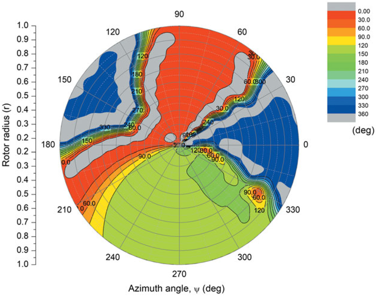
Figure 11. AOA distribution on the rotor disc at αs = 2°, θ 0 = –13.25°, B1 = –15, V = 700ft/ s.
To check the local aerodynamic coefficients, Figs. 12 and 13 are introduced. The retreating blade has highly negative lift coefficients (reddish area), and the advancing blade is in around zero lift angle (greenish area). Bear in mind that, in this condition, the negative lift coefficient signifies upward lift. The drag coefficient distribution shows the entirety of the role of the retreating blade in Fig. 13. Whereas the advancing side has minimum drag coefficients (reddish area), the retreating side has a high drag distribution (greenish and blue area).

Figure 12. Lift coefficient distribution on the rotor disc at αs = 2°, θ 0 = –13.25°, B1 = –15, V = 700ft/ s.

Figure 13. Drag coefficient distribution on the rotor disc at αs = 2°, θ 0 = –13.25°, B1 = –15, V = 700ft/ s.
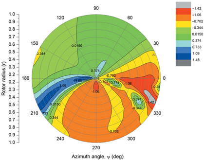
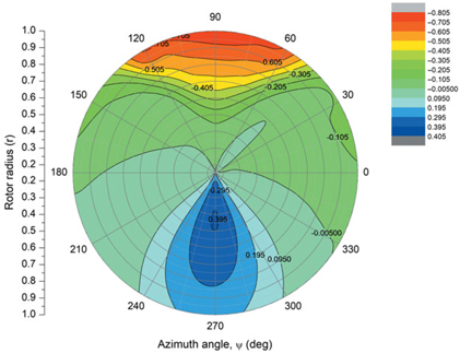
The torque contribution of this drag distribution can be found in Fig. 14. The blue and greenish retreating side has positive values, and the reddish advancing side has negative values in that a positive value indicates a rotating torque and negatives indicates an anti-rotating torque. Two interesting distributions are introduced at the end of this section. One is the induced velocity distribution on the disc, while the rotor reaches the quasi-static state. In every integrating time step, the induced velocity field is refurnished, and this interesting distribution can be seen in Fig. 15. As shown in the figure, the upwash is present around the forward portion of the disc, whilst the strong downwash is created in the rear portion of the disc (the positive value downward).

Figure 14. Non-dimensionalised torque distribution on the rotor disc at αs = 2°, θ 0 = –13.25°, B1 = –15, V = 700ft/ s.

Figure 15. Induced velocity distribution on the rotor disc at αs = 2°, θ 0 = –13.25°, B1 = –15, V = 700ft/ s.
Figure 16 shows the flapping angle distribution for azimuthal positions. The number one blade is in the basic position (azimuthal angle of zero) at the start of all simulations. Therefore, the forming azimuthal positions of the No. 1 blade and the phase differences of blades are reasonable. The flapping motion is shown as higher harmonics and this might be interrelated with the lift and drag distributions on the disc, as shown in Figs. 12 and 13. The flap response is highly dependent on the aerodynamic forces as an excitation and damping. Then the aerodynamics are compressibility dominant on the advancing side and boundary layer separated flow dominant on the retreating side which was provided by look up table. Furthermore, the simulated rotor blade has high moment of inertia and high longitudinal cyclic pitch angle was given. Regarding these conditions, the higher harmonics of flap response is possible. Further investigations are required for the flapping dynamics of similar cases.

Figure 16. Flapping angle variation of blades according to the azimuthal angle at αs = 2°, θ 0 = –13.25°, B1 = –15, V = 700ft/ s.
3.5 Discussion
We define the meaning of ‘the adverse cyclic and collective pitch input’ in this study. Literally, this is equivalent to reducing the forward airspeed of helicopter: pulling back the cyclic lever and pushing down the collective lever. Accordingly, ‘increasing the adverse cyclic and collective pitch’ means that the collective pitch lever is pushed down further, and the cyclic pitch lever is pulled back more. This is not a common practice when increasing airspeed in helicopter operation, in the sense that the collective lever must be pulled up and the cyclic be pushed forward. However, we are not discussing a helicopter in this paper. The focuses of the study are how an autorotating rotor should be controlled and how its performance is changed. If the rotor itself is to be controlled, the cyclic and collective pitches could be both control inputs along with the shaft angle. Conclusively, ‘the adverse cyclic and collective pitch input’ in autorotation is defined as a method for controlling the rotor in increasing airspeed.
A separate device typically provides forward propulsion in autorotational flight, although an off-and-on type shaft power transforming forward thrust might be possible. In either case, it is assumed that propulsion is very controllable. Only the longitudinal cyclic input was simulated. Looking inside the control of the aircraft itself, an alternative control device can be used along with a longitudinal cyclic rotor control, namely, horizontal tail control. Of course, the longitudinal cyclic pitch is a variable of the longitudinal stability of the rotorcraft. In fast flight, if the rotorcraft is equipped with horizontal and vertical control surfaces as well as forward propulsion, then the collective pushes, the cyclic backs, and the throttle opens, while the control wheel (horizontal tail surface) pushes forward. A synthesised control system was already fabricated in XH-59A (Ref. Reference Ruddell3), only the control logic would be different from that. We will not add more commentary here because the systematic consideration is beyond this study.
The full-scale rotor that was simulated in this study has an identical configuration and solidity to the BO-105 helicopter rotor. Since the scale is similar to the BO-105 helicopter, the rotor speed range of 400 rpm and the loading condition of 4600 lbs can be comparative parameters. In this study, the generated more than 3000 lbs of lift might be a relatively large value considering the flight conditions of a shaft angle of 2° and an airspeed of 700ft/s. If we accept the simulation results straightforward, then it means that the combination of counter rotating rotors and convertible jet could be the best configuration for futuristic rotorcraft (configuration of XH-59A might be) — without wing compound, a higher speed and payload than developing coaxial compound helicopter could be possible. Wing and rotor compound transport could secure economic feasibility. However, the control logic would be challenging.
The parameters such as the complicated flow pattern around the blade airfoil, the aeroelasticity of the blade, the compatibility between two-dimensional aerodynamics and inflow theory, the blade vortex interaction, and shock wave dissipation might influence the performance of the rotor quantitatively. Nevertheless, from the perspective of physics and aerodynamics, the new phenomenon shown in this study might exist qualitatively. Wind tunnel tests and sophisticated numerical analyses are required.
4.0 CONCLUSION
Numerical simulations were performed for four variables (cyclic and collective pitches, shaft angle, and airspeed) to observe the characteristic changes in the autorotating rotor. For airspeed, shaft angle, and collective pitch, without cyclic consideration, the collective pitch range becomes narrower with increasing airspeed and decreasing shaft angle. A rotor speed limit boundary line exists in the rotor speed envelopes for three variables. In this case, the compressibility effect of the advancing blade tip restricts the rotor speed at high forward airspeeds, creating a rotor speed boundary line. Rotor performance gradually decreases with increasing airspeed and reducing shaft angle. Combining negative longitudinal cyclic and collective pitch input makes the rotor dynamic at high airspeeds. The rotor speed and thrust increase at low shaft angles and high airspeeds; accordingly, both the rotor lift and lift-to-drag ratio increase. The adverse cyclic and collective pitch effect is prominent at high airspeeds, but the phenomenon appears gradually with changing shaft angles and airspeeds. Phenomenally, the adverse effect is reasonable in terms of physics and aerodynamics. By adjusting the longitudinal cyclic, collective and shaft angles, the complicated and peculiar aerodynamics of the high-advance-ratio rotor can be effectively controlled, and with this, the high-speed capability and performance of the rotorcraft can be notably improved.
ACKNOWLEDGEMENTS
This work was supported by the Korea Institute for Advancement of Technology(KIAT) grant funded by the Korean government (MOTIE: Ministry of Trade, Industry & Energy) (No. 0002431) and the author would like to acknowledge the contribution of Dr. Choi Sung Wook for his analyses of blade airfoil.