


Nomenclature
- 3D
3-dimensional
- 4D
4-dimensional
- alt
altitude
- A/C
aircraft
- ATC
air traffic control
- ATFM
air traffic flow management
- ATM
air traffic management
- CA
total number of the conflict manoeuvres
- CA
collision avoidance
- CD
conflict detection
- CNS
communication, navigation and surveillance
- CP
conflict point
- CPA
closest point of approach
- D
diameter of protected cylinder
- DDR2
demand data repository 2
- DST
decision support tool
- ECAC
European Civil Aviation Conference
- EDE
ecosystem deadlock event
- ET
ecosystem time
- FL
flight level
- H
height of protected cylinder
- I
number of conflict subintervals
- lat
latitude
- LAT
look-ahead time
- long
longitude
- m
type of manoeuvre
- M
number of manoeuvres
- MTCD
mid-term conflict detection
- N A
number of aircraft
- N STI
number of spatiotemporal interdependencies
- NextGen
Next Generation Air Transportation System
- PM
prediction moment
- RBT
reference business trajectory
- s
aircraft state position
- S A
total number of the ecosystem resolutions
- ST
surrounding traffic
- STCA
short-term conflict alert
- STI
spatiotemporal interdependency
- SESAR
Single European Sky ATM Research
- SM
separation management
- SSM
standard separation minima
- t CP
starting conflict moment
- t DE
deadlock event instant
- t Ek
ending moment of the kth conflict subinterval
- t PM
conflict prediction instant
- t Sk
starting moment of the kth conflict subinterval
- TCAS
traffic-alert and collision avoidance system
- TMA
total manoeuvrability of the ecosystem aircraft
- TW
time window
- v
aircraft velocity vector
- τ
checking time rate
1.0 INTRODUCTION
Trajectory deviations in high dense air traffic delimited volumes causes the separation minima infringements in many air traffic control (ATC) sectors. This reduction generates a complexity in the assigned traffic and increases the workload of air traffic controllers, especially at the tactical level( Reference Liu and Hwang 1 ). As a response, several research and development concepts have been carried out to advance the Communication, Navigation and Surveillance/Air Traffic Management (CNS/ATM) technology and meet the principal attributes: safety, capacity and cost-efficiency of operations( Reference Cook, Belkoura and Zanin 2 , Reference Gluchshenko and Foerster 3 ). Based on SESAR (Single European Sky ATM Research) and NextGen (Next Generation Air Transportation System) initiatives( 4 , Reference Enea and Porretta 5 ), it is expected a replacement of the centralised ATC interventions by a distribution of separation management (SM) tasks, relying on advanced decision support tools (DSTs). This foresees important changes in the co-operation, situational awareness and functionalities of the overall ATM system( Reference Prandini, Piroddi, Puechmorel and Brázdilová 6 ).
When a loss of standard separation minima (SSM) between two aircraft occurs, they are considered being in a conflict. For en-route traffic, the SSM in the horizontal plane takes 5 nautical miles (SSMH=5 NM), while in the vertical plane, it is 1000 feet (SSMV=1000ft). An important aspect of the tactical conflict detection (CD) algorithms is the prediction moment (PM), that is, a time instant at which the loss of separation is anticipated. Time measured from this moment until a moment at which two conflicting aircraft reach their closest point of approach (CPA) is denoted as the look-ahead time (LAT). CPA is an estimated 4D point at the aircraft trajectory, at which a 3D distance between two aircraft in conflict reaches its minimum value. Depending on the instant at which a separation minima infringement is predicted (starting conflict moment, t CP), aircraft dynamics and trajectory geometries, the predicted pairwise encounter can be properly handled by an ATC directive, such as speed, heading or altitude change. In Ref. 7, it is reported how major changes in the active aircraft manoeuvrability could potentially induce successive conflicts with neighbouring aircraft and pull them in collision avoidance (CA). CA is the last safety net layer( Reference Kochenderfer and Chryssanthacopoulos 8 ), which is fired because the conflicting aircraft following their trajectories, or performing any feasible manoeuvre, would not preserve the SSM. In these situations, the aircraft separation falls for other safety requirements and is delegated to the safety systems on-board aircraft( Reference Sheperd, Cassell, Thapa and Lee 9 ). One of such systems is Traffic alert and Collision Avoidance System (TCAS). TCAS, as an airborne autonomous system, demonstrates excellent performances for pairwise aircraft encounters but, unfortunately, suffers from a lack of a performance logic owing to well-reported induced collisions from the surrounding traffic scenarios( Reference Bennett 10 ). Moreover, TCAS resolution advisories are frequently opposite from the ATC procedures and could create a lack of integration between the SM layer at the tactical level, and the CA layer at the operational level( Reference Murugan 11 ). Thus, new research concepts relating a coherent integration of the full safety net are essential.
The aerial ecosystem framework relies on the analysis of spatiotemporal interdependencies between aircraft located in the surrounding traffic of a pairwise conflict that will lead to a trajectory amendment. By checking the manoeuvrability impact of any aircraft that could be affected by a pairwise conflict resolution, it is possible to predict an operationally emergent behaviour of the surrounding traffic and identify a subset of the trajectory amendments that will not cause a negative domino effect with neighbouring aircraft. At a technological level, the proposed ecosystem concept( Reference Radanovic, Piera, Koca and Nieto 12 ) relies on multi-agent technology( Reference Premm and Kirn 13 , Reference Ramasamy, Sabatini, Gardi and Kistan 14 ), in which agents represent a set of aircraft inside a computed airspace volume, with a trajectory-amendment decision-making capability, whose trajectories are causally involved in the safety event. Each time a conflict is detected, an aerial ecosystem is initialised with the aircraft involved in a pairwise conflict, and it engages all the surrounding aircraft whose trajectory segments could be affected by a trajectory amendment of a conflict aircraft during the LAT. The set of spatiotemporal interdependencies (STIs) between ecosystem aircraft is analysed in this paper to evaluate the extra capacity to support a seamless transition between the SM and CA safety layers. The STI identification is computed timely in advance by applying the proper operational metrics at specific time instances, preceding the conflict event. The concept supports the trajectory-based operations by discretisation of the 4D trajectories and considers an operational environment in the en-route airspace, above FL245, within a LAT of 300 s. Figure 1 illustrates an example of the ecosystem creation where A/C1 and A/C2, being in predicted conflict, identify the surrounding traffic (ST) aircraft, namely A/C3 and A/C4, by applying certain avoidance manoeuvers, m2 and m4 (the manoeuver types are further explained in Section 3).

Figure 1 Ecosystem creation.
The ecosystem services enhance co-operative aircraft interactions and resolution decisions before the conflict evolves into an ecosystem deadlock event (EDE)( Reference Li 15 , Reference Misra 16 ). This event is characterised by a time instant at which an induced collision could emerge as an effect of a trajectory amendment. EDE depends on the geometric profiles of the ecosystem trajectories, the aircraft closure rates and performances. A time frame between the ecosystem creation moment and the EDE instant is used by the ecosystem members to negotiate their conflict resolutions. This negotiation could be implemented by the multi-agent ontology framework( Reference Hadzic, Wongthongtham, Dillon and Chang 17 ), in which each aircraft is enhanced by a self-governed capability to follow its own performance model to identify a preferred resolution. This technology provides right support in the negotiation interactions, aiming to reach a timely resolutions consensus and avoiding the ATC intervention before EDE, which does not consider the airspace users’ preferences.
Developed ecosystem algorithms provide a robust methodology and the functionalities, intended as an integrated ATC-supporting tool. The tool is to be operable in the en-route airspace, at the tactical level, for a relatively short-time separation provision. The main outcomes for ATC are the computation of compulsory resolutions at the different ecosystem timestamps, a loose measure of the complexity of the ecosystem and a set of feasible resolutions that could be shared with the airspace users involved in the ecosystem for ranking preferences.
This article examines an extra capacity in the generation of the resolution trajectories when a time criticality is threatening the decision-making ability of the ecosystem aircraft. This criticality is expressed by the ecosystem EDE that differently occurs in the traffic scenarios with different complexities. The complexity of those scenarios is based on the concept of aerial ecosystems. At a tactical level, an aerial ecosystem presents a set of aircraft, having an autonomous decision-making capability, that are flying inside certain airspace volume, whose trajectories are causally involved in the safety event-detected conflict. Those aircraft strive to the formation of a cost-efficient separation management by exploring the preferred resolutions and actively interacting with each other. This study focuses on computation of a decreasing rate in the amount of potential resolutions as well as EDE from the identified STIs among trajectories. EDE is characterised by a time instant at which at a total number of the ecosystem solutions takes the zero value. Through simulations of two generated ecosystem, extracted from a real traffic scenario, the paper illustrates the relevant properties inside the structure of the ecosystem interdependencies and discusses an available time capacity in the resolutions process of the ecosystem aircraft. The simulation cases of two ecosystems extracted from a real traffic scenario have been conducted and analysis of the potential resolutions capacity has shown some operational aspects, but also the limitations. These limitations will be subject to further research steps through the implementation of the multi-agent systems ontology, as a significant enabler.
In addition to this introductory section, the paper comprises additional four sections. Section 2 is dedicated to the problem definition. Section 3 describes the computational framework for identification of the STIs from the ecosystem creation algorithm and analytical model for a potential resolution capacity (decreasing rate in the number of potential resolutions) and the EDE. Section 4 discusses the simulation results and comments on the time capacity for both ecosystems, while the concluding remarks and directions for the follow-up research are given in Section 5.
2.0 Problem definition
This section illustrates two key aspects of the conflict resolution analysis in the complex traffic environments. Their justification requires the new quantitative methods to enhance present safety nets.
2.1 Conflict interval for the pairwise encounter
The tactical level within air traffic flow management (ATFM) is timely framed between two ATC thresholds: mid-term conflict detection (MTCD), that activates approximately 15min before the closest point of approach (CPA) between two aircraft, and short-term conflict alert (STCA), that is triggered around 120s before the CPA( Reference Chaloulos, Roussos, Lygeros and Kyriakopoulos 18 ). After STCA, two aircraft in conflict could potentially enter a CA layer that is characterised by a non-ATC separation provision, but an autonomous airborne safety system, such as TCAS( Reference Tang, Piera and Guasch 19 ). Therefore, new research lines are required towards the development of the collaborative and decentralised tactical aerial system, on which both human behaviour and automation will be fully aligned. That envisages an operational integration of the safety procedures in such a way that any pair of aircraft involved in a conflict, together with surrounding aircraft, behave as a stable conflict-free air traffic system. Furthermore, the integration should be characterised with the critical information on the feasible resolution trajectories proposed through the development of the airborne and ground-based DSTs( Reference Vela, Vela and Ogunmakin 20 ).
Figure 2 describes the conflict process between two aircraft, projected in the horizontal and vertical plane. The conflict between aircraft A/C1 and A/C2 (Fig. 2(a)) starts when they reach the waypoints CP1 and CP2, and ends when fly over CP’1 and CP’2, respectively. At CPA1 and CPA2, the aircraft come to the shortest conflict distance. The starting conflict moment is approximately close to the STCA threshold. In most cases, it is detected after STCA (CP-I), but it can also occur before (CP-II) when the closure rates are lower and the geometric configuration of trajectories is more complex. Detection of this moment is essential for coherent transition from separation management to collision avoidance. The conflict interval ends up at CP’ (Fig. 2(b)). A very frequent case in a geometry of the aircraft encounters is that a CPA instant presents also the starting conflict moment (Fig. 3). In this case, PM is advanced 300s before the beginning of the conflict.

Figure 2 (Colour online) Conflict process for pairwise encounter; transition from SM to CA.

Figure 3 (Colour online) The conflict interval where the CPA and CP moments overlap.
Therefore, a proper detection of the conflict interval, for the pairwise encounter, is essential for the ecosystem conflict management. The starting conflict instant must be a referent moment from which the EDE instant can be computed, depending on the complexity of the ecosystem scenario, i.e. the number of aircraft and a geometry of their trajectories (Fig. 4). In this sense, the ecosystem life time (ET) is defined as time difference between EDE and PM. A longer LAT provides an extra time for the analysis of all STIs and enhances a co-ordinated set of conflict resolution manoeuvers; however, it also increases considerably the uncertainty in the trajectories and the amount of unnecessary ecosystem members. On the other hand, a reduction of the LAT could drastically affect the safety of planned operations. Thus, a LAT of 300 s allows the use of aircraft state variable information to represent the ecosystem trajectories by segments with a low uncertainty.

Figure 4 (Colour online) EDE positioning within the LAT and ET determination.
2.2 Ecosystem evolution and deadlock event
The ecosystem evolution towards a determined EDE is characterised by a continuously decreasing rate in the number of potential resolutions that could be applied during the ecosystem life time. Figure 5 illustrates the ecosystem evolution in the vertical plane over three time-windows, TW1, TW2 and TW3. Each subsequent window is a sub-window of the previous one. TW3 denotes a CA window whose edges present the EDE moment. Aircraft reaching this ecosystem window on their Reference Business Trajectories (RBTs) would not be subject to the ATC separation provision, but the TCAS activation. Therefore, any co-ordinated (co-operative) manoeuvers of the aircraft that would provide a conflict-free ecosystem resolution, with respect to the SSM, must be performed before entering TW3.

Figure 5 (Colour online) Ecosystem evolution towards EDE.
Figure 6 shows a theoretical decreasing rate in a number of the conflict-free solutions, denoted with S(t), over the LAT. The values for S(t) have been taken as an example to illustrate a higher drop in the amount of solutions occurring until the TW1, and then follow-up with lower decreasing rate until the TW2. S(t) is approaching to the value “0” when the ecosystem enters the TW3. The time threshold for entering TW3 presents a CP instant for a detected pairwise conflict. In most cases, their order of magnitude is higher, that depends on the manoeuverability discretisation supported by the technology, the ecosystem size (the number of involved aircraft) and the STI structure among the trajectory segments.

Figure 6 (Colour online) Rate of change in the number of resolutions.
3.0 Computational framework
This section describes the procedure for the STI identification and its utilisation on the analytical computation of the EDE. A short reference to the ecosystem generation has been provided with an aim at introducing the manoeuverability criteria that could be maintained for the resolutions generation.
3.1 State-based CD and ecosystem creation
For computation of the starting conflict moment, t CP, there has been implemented a Eucledean state-based CD algorithm. As developed in Ref. 21, the algorithm simplifies the methodology referring to the case of two aircraft in conflict, A and B. Their states can be described by positions s A and s B, and their velocity vectors by v A and v B, respectively. Projections of the aircraft A position along axes are denoted with s Ax, s Ay and s Az, while projections of its velocity vector are marked with v Ax, v Ay and v Az, respectively. Each aircraft is surrounded by an imaginary volume called the protected zone. It defines a minimum separation distance between aircraft. The protected zone in a 3D space takes a shape of a flat cylinder with diameter D and height H. Therefore, the imaginary cylinder around the aircraft A is defined by the set of points (x, y, z) satisfying the conditions:
 $$\sqrt {(x{\minus}s_{\rm Ax})^{2} {\plus}(y{\minus}s_{\rm Ay})^{2} } \,\lt\,{D \over 2}$$
 $$\left| {z{\minus}s_{\rm Az}} \right|\,\lt\,{H \over 2}$$
The minimal separation distance is considered here as SSM, which means:
 $${\rm SSM}_{{\rm H}} {\equals}{D \over 2}{\equals}5\,{\rm NM},$$
and
$${\rm SSM}_{{\rm H}} {\equals}{D \over 2}{\equals}5\,{\rm NM},$$
and
 $${\rm SSM}_{{\rm V}} {\equals}{H \over 2}{\equals}1000$$
ft. In a general context, the protected zone of the aircraft A is defined as a set of points, P
A, that satisfy
$${\rm SSM}_{{\rm V}} {\equals}{H \over 2}{\equals}1000$$
ft. In a general context, the protected zone of the aircraft A is defined as a set of points, P
A, that satisfy
 $$P_{\rm A}{\equals}\left\{ {x\left| {\left\Vert {s_{\rm A}{\minus}x} \right\Vert\,\lt\,{1 \over 2}} \right.} \right\}$$
where ∥.∥ denotes a norm vector. In the case of the cylinder of diameter D and height H, the norm is defined as
 $$\left\Vert {\left( {x,y,z} \right)} \right\Vert{\equals}{\rm max}\:\bigg({{\sqrt {x^{2} {\plus}y^{2} } } \over D}\:,\:{{\,\mid z \mid\,} \over H}\bigg)$$
Using a norm expression, it can be defined as a distance between aircraft and, as a result, a loss of the SSM. The distance between the aircraft A and B is defined as
 $$\Delta ({\rm A,\:B}){\equals}\,\mid \mid s_{\rm A}{\minus}s_{\rm B}\mid\mid\,$$
A and B are in loss of separation if and only if Δ (A, B)<1. One of the assumptions for the ecosystem creation is a linearity. At the future time instant: t, the state prediction A(t) from the current position can be expressed as
 $$s_{\rm A}\left( t \right){\equals}s_{\rm A}{\plus}t\:v_{\rm A}$$
 $$v_{\rm A}(t){\equals}v_{\rm A}$$
CD is a predicted loss of separation between aircraft A and B within LAT. A and B are in conflict if there is a predicted instant t CP, at which an achieved distance between the aircraft will be less than 1:
 $$\Delta ({\rm A}(t_{\rm CP}),\,{\rm B}(t_{\rm CP}))\:\:\,\lt\,1$$
Once the conflicts are detected, duration of the conflict intervals is checked by sampling the trajectories with 1-s rate, and comparing the shortest distances between the points of two trajectories at each instant with the SSM criteria (SSMH and SSMV). When the inter-distance exceeds either SSMH or SSMV (or both) the conflict interval ends in the moment t CP The ecosystem creation procedure has been elaborated in Refs Reference Radanovic, Piera, Koca and Nieto12 and Reference Radanovic and Eroles22. This algorithm determines all cluster members as surrounding traffic aircraft for which the loss of SSM with any of two conflicting aircraft would occur if this aircraft performs a given avoidance manoeuver at any moment during LAT (Fig. 1). Considerably, the ecosystem creation is a spatiotemporal category as the applied manoeuver generates conflict subintervals with the surrounding aircraft. Manoeuverability is applied in both horizontal and vertical planes (Fig. 7) using a certain set of parametric values to identify those surrounding traffic aircraft that should be considered ecosystem members:
∙ m 1 : left heading change with a deflection angle of +30°;
∙ m 2 : right heading change with a deflection angle of −30°;
∙ m 3 : climb at a vertical rate of +1000 ft/min, and a flight path angle of +2°;
∙ m 4 : descent at a vertical rate of −1000 ft/min, and a flight path angle of −2°.

Figure 7 Identification of two ST aircraft; (a) A/C3 by left heading manoeuver of A/C1 and (b) A/C4 by climb amendment of A/C1.
3.2 STI identification and EDE computation
The STI identification refers to the computation of the time windows for each ecosystem aircraft, inside which any potential co-operative or non-co-operative, horizontal or vertical, manoeuver could produce a loss of the SSM. Those windows are subintervals of LAT and the total number of conflict manoeuvers within each window is obtained as per defined time rate (by default, 1s) along each RBT segment. Figure 8 shows an example of the conflict subinterval generated using left heading change. Conflict subinterval no. 1 (CI1) denotes the period in which A/C1 performing a given manoeuver generates continuous conflict with A/C3.

Figure 8 Conflict subinterval for a single RBT applying a deflection angle of +30°.
The number of STIs (NSTI) between pairs of aircraft is obtained using four types of avoidance manoeuvers, explained above (m 1 , m 2 , m 3 and m 4 ), and one additional, m 0 : RBT follow-up. m 0 means that an aircraft decides to continue flying over its RBT in a given moment. In this study, therefore, five types of manoeuvers are counted for, i.e., M=5. However, further research might introduce more manoeuvers (i.e., holding turns, regulated speed modifications among others) in the analysis. Each interdependency contains one or more conflict subintervals, and a total number of the conflict subintervals (I) within one ecosystem must satisfy the following condition:
 $$I\leq {{N_{\rm A}\:(N_{\rm A}{\minus}1)\:} \over 2}\:M^{2} $$
N A denotes the number of ecosystem members, and M 2 is a derived property that presents the total number of manoeuvering combinations applied to one pair of aircraft. An example of the STI structure is presented in Table 1. It consists of the STI identifier, a combination of two interdependent flight identifiers, manoeuvering combination and conflict subinterval. t Sk presents the starting instant of the conflict subinterval k for a pair of the ecosystem aircraft, while t Ek denotes the ending moment, t Sk<t Ek, k ∈[1, I]. One STI for one aircraft pair might have more conflict subintervals generated due to different manoeuvering combinations. Figure 9 illustrates an ecosystem example described in Table 1.

Figure 9 (Colour online) Spatiotemporal interdependencies for the given ecosystem with three members.
Table 1 Example of the STI structure

From Fig. 4, it can be expressed LAT and ET
 $${\rm LAT}{\equals}t_{\rm CP}{\minus}t_{\rm PM}$$
 $${\rm ET}{\equals}t_{\rm DE}{\minus}t_{\rm PM}$$
where t CP, t PM and t DE present timestamps of predicted pairwise conflict, prediction moment and deadlock, respectively. With an objective to compute t DE, in this study, the ecosystem solutions are treated as three-fold:
1. Co-operative mechanism: All aircraft involved in an ecosystem resolution amendment should initialise the manoeuver at the same time instant. Therefore, the resolution capacity at a certain timestamp, and in terms of the available time until the system deadlock, is compressed.
2. The resolution manoeuvers must correspond to the avoidance manoeuvers (Table 1) with a certain discretisation of the heading and vertical rate. Analysis of the ecosystem solution with a spectrum of the manoeuvering values is out of scope in this paper. The computation of the deadlock event would require a more thorough state-space-search technique.
3. The resolution manoeuvers are considered potential, as some of them might be acceptable and other unacceptable by the airspace user. The paper only analyses a potential time-space capacity for resolutions, and the acceptability is not considered since it highly depends on the airspace users’ business models.
Nevertheless, the STI algorithm outputs the ecosystem conflict structure for each interdependency, meaning that an ecosystem solution is not possible at a time instant belonging to any of the conflict subintervals. In other words, any time window in which no interdependency exists is treated as a potential solution interval. Therefore, it can be concluded that a total number of ecosystem resolutions from the given time instant t, t∈[t PM, t CP), to t DE equals to a difference between a theoretical number of the ecosystem manoeuvers and a total number of the conflict manoeuvers, succeeding this instant, provided that the manoeuverability checks are performed with the constant time rate. Therefore, the theoretical number of the ecosystem manoeuvers is defined as
 $${\rm {TM}_A}(t)\:{\equals}\:{{M^{{N_{\rm A}}} } \over \rtau }\:(t_{\rm CP}{\minus}t)$$
where τ presents checking time rate (1 s, by default). In addition, for ∀t Sk∈[t PM, t CP), ∀t Ek∈(t PM, t CP], a conservative bound of conflict manoeuvers that cannot be flown due to STIs with surrounding aircraft is computed as
 $$C_{\rm A}(t){\equals}{{M^{{(N_{\rm A}{\minus}2)}} } \over \rtau }\:\mathop{\sum}\limits_{k{\equals}1}^I {[t_{\rm Ek}{\minus}{\rm max}\:(t_{\rm Sk},\:t)]} $$
and the number of potential ecosystem resolutions
 $$S_{\rm A}(t){\equals}{\rm TM_A}(t){\minus}C_{\rm A}(t){\equals}{{M^{{(N_{\rm A}{\minus}2)}} } \over \rtau }\:\:\Bigg(M^{2} (t_{\rm CP}{\minus}t){\minus}\mathop{\sum}\limits_{k{\equals}1}^I {[t_{\rm Ek}{\minus}{\rm max}\:(t_{\rm Sk},\:\:t)]} \Bigg)$$
The maximum number of solutions is obtained in the moment of the ecosystem creation, i.e. t=t PM
 $$S_{\rm Amax}{\equals}{{M^{{(N_{\rm A}{\minus}2)}} } \over \rtau }\Bigg(M^{2} (t_{\rm CP}{\minus}t_{\rm PM}){\minus}\mathop{\sum}\limits_{k{\equals}1}^I {[t_{\rm Ek}{\minus}t_{\rm PM}]} \Bigg)$$
S A(t) is characterised by a decreasing rate in the time evolution. Finally, the deadlock event occurs when the number of the ecosystem solutions reaches the 0-value, i.e., S(t)=0:
 $$M^{2} (t_{\rm CP}{\minus}t_{\rm DE}){\minus}\mathop{\sum}\limits_{k{\equals}1}^I {[t_{\rm Ek}{\minus}t_{\rm DE}]} {\equals}0$$
Expression (16) computes the value of t DE that corresponds to TW3, illustrated in Figs 5 and 6.
4.0 Analysis of simulation results
This section provides relevant results obtained from simulations of two ecosystems. The traffic scenario used for this purpose was DDR2,Footnote 1 s06.m1 model that comprises 4D flight plans( Reference Wandelt and SUN 23 ). The analysed traffic was dated on 24/08/2017 within the ECAC (European Civil Aviation Conference) airspace, with the total number of 36,095 flights during the day. Then, a traffic scenario was created by extracting of this traffic volume over the time interval 16:00–19:00, and filtering by altitude, above FL245 (the en-route airspace). The scenario counted for 9,698 flights.
From the traffic simulation, 2,237 pairwise conflicts have been identified, and two of them have been selected for analysis of the ecosystem creation and resolutions generation. The first ecosystem consists of three aircraft, while the second one was composed of four. Tables 2 and 3 provide the structure of the trajectory segments for the aircraft inside both ecosystems (for simplicity, instead of the flight identifiers – digits – there has been used an abbreviation “A/C#”). The abbreviations “lat”,”long” and “alt” present 3D spatial co-ordinates: latitude, longitude and altitude, respectively. The index “1” denotes the co-ordinates of the first 4D point, while “2” express the second one. Latitude and longitude are expressed in decimal degrees, altitude in feets and time in seconds. The time values are given in the accumulated seconds counted from the beginning of day.
Table 2 Ecosystem 1 – trajectory segments

Table 3 Ecosystem 2 – trajectory segments

For a better understanding of computation of the number of resolutions, the timestamps are converted to LAT interval (300-s-periods), taking
∙ time-1=t PM=0 s – for both ecosystems,
∙ time-2=t CP=298.00 s – Ecosystem 1,
∙ time-2=t CP=218.49 s – Ecosystem 2.
Figures 10 and 11 (a, b and c) graphically describe the ecosystems in 3D (latitude–longitude–altitude) and 2D projections (longitude–latitude and time–altitude).

Figure 10 (Colour online) Ecosystem 1 in (a) 3D projection (latitude–longitude–time), (b) 2D planar projection (latitude–longitude) and (c) 2D vertical projection (time–altitude).
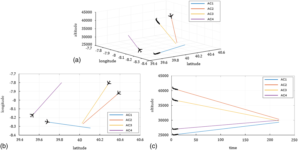
Figure 11 (Colour online) Ecosystem 2 in (a) 3D projection (latitude–longitude–time), (b) 2D planar projection (latitude–longitude) and (c) 2D vertical projection (time–altitude).
The simulation runs have output the main properties related to the STI structure (Table 4) while Figure 12 describes the potential resolution capacity for Ecosystems 1 and 2.

Figure 12 (Colour online) Decreasing rate in the number the resolutions of (a) Ecosystem 1 and (b) Ecosystem 2.
Table 4 STI properties

Looking at the values in Table 4, it can be observed that Ecosystem 1 (Ecosystem ID column) with three aircraft (N A column) generated three interdependencies (N STI column), while Ecosystem 2 with four aircraft generated four interdependencies. The interdependencies within Ecosystem 1 produced 19 conflict subintervals in total (I column), while in the case of Ecosystem 2 there were 33. The maximum number of solutions in the moment of Ecosystem 1 creation is 20,990 (S Amax column), and, in the case of Ecosystem 2 creation, this number goes to 50,291 that initially provides more resolution capacity to Ecosystem 2. However, due to a significantly higher number of the conflict subintervals and their longer durations, Ecosystem 2 reaches the deadlock moment faster (t DE=149.47 s) comparing to Ecosystem 1 (t DE=219.17 s). The values for t DE are provided with respect to the ET interval (t DE column). As the cumulative timestamps, those values correspond to 60,848.17 and 67,128.47 s for Ecosystems 1 and 2, respectively.
Figure 12(a) describes the resolutions capacity of Ecosystem 1 over its time, which equals to LAT, i.e., ET=LAT since t CP=300 s. In the case of Ecosystem 2 in Fig. 12(b), the capacity is measured within a time interval of 218 s (ET=218). Obviously, in the latter case, the starting conflict point does not overlap with the closest point of approach (300 s after the ecosystem prediction moment) due to the operational factors, such as a relative geometry of the ecosystem trajectories and aircraft dynamics (position, velocity and flight mode). The solutions curve in the first case is decreasing at a lower rate with respect to the distribution (allocation) of the conflict subintervals produced by the aircraft interdependencies, with the distinction that, after 170 s, the reaming number of solutions drops at a higher rate. However, Ecosystem 1 still reaches deadlock after approximately 219 s, which is notably earlier from t CP (80 s before). Regarding Ecosystem 2, the structure of the conflict subintervals is quite specific. The solutions curve is slightly maintained first 50 s, and then decreases at a quite low rate until 90 s. Because of the fact that frequency and duration of induced conflict subintervals is dominant after 100 s, the curve showed a drastically negative trend by a drastic drop in the capacity until the deadlock moment, that occurred approximately after 150 s. Based on the results presented in Table 4 and illustrated in Fig. 12, it can be concluded that both ecosystems faced a relatively shorter time in resolution with respect to the available times. The t DE values for both ecosystems are significantly “shifted back” with respect to the t CP values, as the complexities of evolving trajectories close to these instants are significantly increased. At those moments, no combination of the co-ordinated manoeuvers would remove the SSM infringement.
To co-operatively resolve the conflicts before collision avoidance, the aircraft are frequently required to align their velocities and adjust their inter-distances for computation of the moment for triggering the co-operative resolutions. On the contrary, the ecosystem concept elaborated in this paper extends the time horizon providing more decision capacity at the SM level. The aircraft are aware of a potential EDE while flying to the CPA, and given a possibility to interactively negotiate the solutions, not requiring a priori any adjustment in velocity or heading and following the trajectories as approved. A time frame between the ecosystem prediction moment and a moment where ATC issues the compulsory directives is reserved for the ecosystem members to negotiate the system solutions. As indicated in the paper (Section 1), this negotiation might be implemented through the multi-agent ontology, in which each aircraft, as an intelligent agent, is enhanced by a self-governed capability to follow its own performance model, identify a preferred resolution, and try to impose it to other members. This framework provides the right support in the negotiation interactions, aiming to reach a timely resolutions consensus and avoiding the ATC directives before the EDE, which do not always consider the airspace users’ preferences.
A decreasing rate between the available resolution capacity and elapsed time, expressing a potential path in negotiations among the aircraft, indicates that each missed moment in reaching an agreement among them reduces the number of remaining conflict-free solutions. Moreover, identification of a higher number of the causally involved aircraft into enlarged ecosystem volume provides an opportunity for an efficient modelling of the optimal trajectories, usually with the minimal deviations, and not compromising the separation criteria.
5.0 Conclusion and follow-up research
This article relies on the previous research on the ecosystem creation algorithm, trying to identify the potential extra capacity in the search space of the conflict-free resolution manoeuvres. The main driver in this creation is the state-based CD in a pairwise aircraft encounter and its time instants, the prediction moment and starting conflict moment. The computational framework has presented the baseline in the identification of the STIs, expressing the structure of the conflict subintervals as a product of the potentially combined manoeuvres. The model has further included the analytical computation of decreasing rate in the amount of potential resolutions, as well as the ecosystem deadlock event in which this amount has reached the zero value. The study has shown a significance in providing the time capacity for a set of certain manoeuvres, at the operational level, when a severity of the conflict situation occurs very rapidly. A decreasing rate of the available ecosystem resources and an elapsed time described a potential path in a thorough analysis of resolution dynamics, meaning that each missed moment in making a resolution agreement induces less number of the conflict-free manoeuvres. The results, obtained through analysis of two simulated ecosystems, illustrated the cases of the variable resolution capacity that decreases over time at a different rate. With an increased ecosystem size and diverse trajectory geometries, the interdependencies structure becomes larger which produces less resolution capacity and a shorter ecosystem time. Finally, the ecosystem runs out of capacity at a certain time instant, which shows a time-critical nature of the ecosystem, where timely-advanced decision provides more flexible and resilient solution.
Further research is considered as multi-directional: analysis of multi-threat conflicts with respect to the time to CPA, and improving the computational performances. Moreover, an improvement in the ecosystem resolutions will focus on a multi-agent technology for simulation of the aircraft interactions during the negotiation intervals. That will provide more reliability in the solutions search space. Another task will be directed towards the generation of the resolution segments, based on the concept of performance-based operations. The main objective will be the computation of the tactical waypoints and definition of modelling elements that could provide smooth transition from the conflict-free amendments. The main criteria in the selection of the ecosystem solutions will be rather feasibility than optimality. Nevertheless, the early resolution agreements shall guarantee the smallest deviations from the RBT segments.
Acknowledgements
This research is partially supported by the H2020 Research and Innovation Programme, the project: “Adaptive self-Governed aerial Ecosystem by Negotiated Traffic – AGENT” (Grant agreement no. 699313), and the national Spanish project: “Automated Air Traffic Management for Remotely Piloted Aircraft Systems” (Ref. TRA2017-88724-R). Opinions expressed in the article reflect the authors’ views only.


