


1. Introduction
Singular and switching stochastic control problems have been of great research interest in control theory owing to their applicability to diverse problems of finance, economy, biology, and other fields; see, e.g., [Reference Kelbert and Moreno-Franco12, Reference Pham16] and the references therein. For that reason, new techniques and problems are continuously being developed. One of these problems, called a mixed singular/switching stochastic control problem, concerns the application of both singular and switching controls in an optimal way on some stochastic process that can change regime. Within a regime, a singular control is executed.
This paper is mainly concerned with determining the regularity of the value function in a mixed singular/switching stochastic control problem for a multidimensional diffusion with multiple regimes on a bounded domain. Our study is focused on the stochastically controlled process
 $\big(X^{\xi,\varsigma},I^{\varsigma}\big)$
that evolves as
$\big(X^{\xi,\varsigma},I^{\varsigma}\big)$
that evolves as

where
 $X^{\xi,\varsigma}_{0}=\tilde{x}\in\overline{\mathcal{O}}\subset\mathbb{R}^{d}$
,
$X^{\xi,\varsigma}_{0}=\tilde{x}\in\overline{\mathcal{O}}\subset\mathbb{R}^{d}$
,
 $I^{\varsigma}_{0-}=\tilde{\ell}\in\mathbb{I}\,:\!=\,\{1,2,\dots,m\}$
,
$I^{\varsigma}_{0-}=\tilde{\ell}\in\mathbb{I}\,:\!=\,\{1,2,\dots,m\}$
,
 $\tilde{\tau}_{i}\,:\!=\,\tau_{i}\wedge\tau$
, and
$\tilde{\tau}_{i}\,:\!=\,\tau_{i}\wedge\tau$
, and
 $\tau$
represents the first exit time of the process
$\tau$
represents the first exit time of the process
 $X^{\xi,\varsigma}$
from the set
$X^{\xi,\varsigma}$
from the set
 $\mathcal{O}$
. Here
$\mathcal{O}$
. Here
 $W=\{W_{t}\,:\,t\geq0\}$
is a k-dimensional standard Brownian motion. The pair
$W=\{W_{t}\,:\,t\geq0\}$
is a k-dimensional standard Brownian motion. The pair
 $(\xi,\varsigma)$
is a stochastic control strategy, defined later on (see (2.1), (2.2)), which consists of a singular control
$(\xi,\varsigma)$
is a stochastic control strategy, defined later on (see (2.1), (2.2)), which consists of a singular control
 $\xi\,:\!=\,(\unicode{x1D55F},\zeta)\in\mathbb{R}^{d}\times\mathbb{R}_{+}$
and a switching control
$\xi\,:\!=\,(\unicode{x1D55F},\zeta)\in\mathbb{R}^{d}\times\mathbb{R}_{+}$
and a switching control
 $\varsigma\,:\!=\,(\tau_{i},\ell_{i})_{i\geq0}$
with
$\varsigma\,:\!=\,(\tau_{i},\ell_{i})_{i\geq0}$
with
 $\tau_{i}$
a stopping time and
$\tau_{i}$
a stopping time and
 $\ell_{i}\in\mathbb{I}$
for
$\ell_{i}\in\mathbb{I}$
for
 $i\geq1$
. The process
$i\geq1$
. The process
 $(\xi,\varsigma)$
is chosen in such a way that it will minimize the cost criterion
$(\xi,\varsigma)$
is chosen in such a way that it will minimize the cost criterion
Under the assumption that there is no loop of zero cost (see (2.7)), one of the main goals of this paper is to verify that the value function
 \begin{equation}V_{\tilde{\ell}}(\tilde{x})\,:\!=\,\inf_{\xi,\varsigma}V_{\xi,\varsigma}\big(\tilde{x},\tilde{\ell}\big),\ \text{for}\ \big(\tilde{x},\tilde{\ell}\big)\in\overline{\mathcal{O}}\times \mathbb{I},\end{equation}
is in
 $\textrm{C}^{0,1}\cap \textrm{W}^{2,\infty}_{\textrm{loc}}$
; see Theorem 2.1.
$\textrm{C}^{0,1}\cap \textrm{W}^{2,\infty}_{\textrm{loc}}$
; see Theorem 2.1.
Previous to this paper, the problem (1.3) has been studied extensively (in both bounded and unbounded set domains) for separate cases: when the process
 $X^{\xi,\varsigma}$
does not change its regime or when the singular control
$X^{\xi,\varsigma}$
does not change its regime or when the singular control
 $\xi$
is not executed on
$\xi$
is not executed on
 $X^{\xi,\varsigma}$
; see, e.g., [Reference Davis and Zervos6, Reference Kelbert and Moreno-Franco12, Reference Lenhart and Belbas13, Reference Pham16, Reference Zhu19, Reference Yamada18] and the references therein. It is natural to study stochastic control problems where both controls are involved, and see how they can be applied.
$X^{\xi,\varsigma}$
; see, e.g., [Reference Davis and Zervos6, Reference Kelbert and Moreno-Franco12, Reference Lenhart and Belbas13, Reference Pham16, Reference Zhu19, Reference Yamada18] and the references therein. It is natural to study stochastic control problems where both controls are involved, and see how they can be applied.
For example, both (singular and switching) controls have been used in the study of interactions between dividend and investment policies. In that context, a firm that operates under an uncertain environment and risk constraints wants to determine an optimal control on its dividend and investment policies (see [Reference Azcue and Muler2, Reference Chevalier, Ly Vath and Scotti4, Reference Chevalier, Gaïgi and Ly Vath3, Reference Ly Vath, Pham and Villeneuve15]). The authors assumed that the cash reserve process of a firm switches between m-regimes governed by Brownian motions with the same volatility but different drifts [Reference Chevalier, Ly Vath and Scotti4, Reference Ly Vath, Pham and Villeneuve15], a two-dimensional Brownian motion with the same stochastic volatility but different stochastic drifts [Reference Chevalier, Gaïgi and Ly Vath3], or different compound Poisson processes with drifts [Reference Azcue and Muler2]. The costs and benefits of switching regimes are made automatically in the firm’s cash reserve and are not considered in the expected returns.
The optimal dividend/investment policy strategy problem mentioned above was studied on the whole spaces
 $\mathbb{R}$
or
$\mathbb{R}$
or
 $\mathbb{R}^{2}$
; see [Reference Azcue and Muler2, Reference Chevalier, Ly Vath and Scotti4, Reference Ly Vath, Pham and Villeneuve15] and [Reference Chevalier, Gaïgi and Ly Vath3], respectively. Using viscosity solution approaches, the authors obtained qualitative descriptions of the value function
$\mathbb{R}^{2}$
; see [Reference Azcue and Muler2, Reference Chevalier, Ly Vath and Scotti4, Reference Ly Vath, Pham and Villeneuve15] and [Reference Chevalier, Gaïgi and Ly Vath3], respectively. Using viscosity solution approaches, the authors obtained qualitative descriptions of the value function
 \begin{equation}\sup_{\zeta}\bigg\{\mathbb{E}_{\tilde{x},\tilde{\ell}}\bigg[\int_{0}^{\tau}\textrm{e}^{-ct}\textrm{d}\zeta_{t}\bigg]\bigg\},\quad\text{with $c>0$ a fixed constant.}\end{equation}
It must be highlighted that the explicit or quasi-explicit solution of the optimal strategy for the first two cases mentioned in the previous paragraph (see [Reference Chevalier, Ly Vath and Scotti4, Reference Chevalier, Gaïgi and Ly Vath3, Reference Ly Vath, Pham and Villeneuve15]) has not yet been found and still remains an open problem. For the case when the cash reserve process switches between m-regimes governed by different Poisson processes with drifts, Azcue and Muler [Reference Azcue and Muler2] proved that there exists an optimal dividend/switching strategy, which is stationary with a band structure.
In addition, Guo and Tomecek [Reference Guo and Tomecek11] studied a connection between singular controls of finite variation and optimal switching problems.
Notice that the mixed singular/switching stochastic control problem proposed in (1.1)–(1.3) is defined on an open bounded domain
 $\mathcal{O}\subset\mathbb{R}^{d}$
, and the costs for switching regimes, represented by
$\mathcal{O}\subset\mathbb{R}^{d}$
, and the costs for switching regimes, represented by
 $\vartheta_{\ell,\kappa}$
, are considered in the functional costs
$\vartheta_{\ell,\kappa}$
, are considered in the functional costs
 $V_{\xi,\varsigma}$
. Additionally, it must be highlighted that our problem is given in a general way, meaning that for every regime
$V_{\xi,\varsigma}$
. Additionally, it must be highlighted that our problem is given in a general way, meaning that for every regime
 $\ell$
, the drift and the volatility of the process
$\ell$
, the drift and the volatility of the process
 $X^{\xi,\varsigma}$
are stochastic, and there are two types of costs:
$X^{\xi,\varsigma}$
are stochastic, and there are two types of costs:
 $g_{\ell}\big(X^{\xi,\varsigma}\big)\circ\textrm{d}\zeta$
when the singular control
$g_{\ell}\big(X^{\xi,\varsigma}\big)\circ\textrm{d}\zeta$
when the singular control
 $\xi$
is exercised, and
$\xi$
is exercised, and
 $h_{\ell}\big(X^{\xi,\varsigma}\big)$
if not. For more details about the cost
$h_{\ell}\big(X^{\xi,\varsigma}\big)$
if not. For more details about the cost
 $g_{\ell}\big(X^{\xi,\varsigma}\big)\circ\textrm{d}\zeta$
, see the next section.
$g_{\ell}\big(X^{\xi,\varsigma}\big)\circ\textrm{d}\zeta$
, see the next section.
The main contributions of this paper are the following:
-
1. We characterize the solution u to a suitable Hamilton–Jacobi–Bellman (HJB) equation, which is closely related to the value function V given in (1.3), as the limit of a sequence of solutions to another system of variational inequalities that is related to
 $\varepsilon$
-penalized absolutely continuous/switching (
$\varepsilon$
-PACS) control problems; see Subsection 2.2.
$\varepsilon$
-penalized absolutely continuous/switching (
$\varepsilon$
-PACS) control problems; see Subsection 2.2. -
2. We give an explicit representation of the optimal strategy of these
$\varepsilon$
-PACS control problems. Then, by probabilistic methods and construction of an approximating sequence of solutions as mentioned previously, we verify that the value function (1.3) and the solution u to the HJB equation (2.9) agree on
$\overline{\mathcal{O}}$
, showing that
$V_{\ell}$
belongs to
$\textrm{C}^{0,1}\big(\overline{\mathcal{O}}\big)\cap \text{W}^{2,\infty}_{\textrm{loc}}(\mathcal{O})$
; see Section 4. -
3. We find explicitly the solution
$\tilde{u}$
to a suitable HJB equation that is related to the value function V given in (1.3), when
$\mathcal{O}=(0,l)\subset\mathbb{R}$
,
$l>0$
, and the parameters of the stochastic differential equation (SDE) (1.1) are given by
$b(x,\ell)=b_{\ell}x$
and
$\sigma(x,\ell)=\sigma_{\ell}x$
for
$x\in(0,l)$
, with
$b_{\ell},\sigma_{\ell}\in\mathbb{R}$
such that
$\sigma_{\ell}>0$
. Additionally,
$c_{\ell}$
and
$g_{\ell}$
are positive constant functions and the running cost
$h_{\ell}$
is taken as
$h_{\ell}(x)\,:\!=\, K_{\ell}x^{\gamma_{\ell}}$
, where
$\gamma_{\ell}\in(0,1)$
,
$K_{\ell}>0$
are fixed; see Section 5.


The rest of this document is organized as follows. In Section 2 we consistently formulate the stochastic control problem studied here (see (2.8)) and give the assumptions for obtaining the main results of this paper, Theorems 2.1 and 2.2. Also we introduce the
 $\varepsilon$
-PACS control problem and its HJB equation (2.19). Then, in Section 3, we introduce a nonlinear partial differential system (NPDS) and give some a priori estimates. Afterwards, using Lemma 3.1, Proposition 3.1, the Arzelà–Ascoli compactness criterion, and the reflexivity of
$\varepsilon$
-PACS control problem and its HJB equation (2.19). Then, in Section 3, we introduce a nonlinear partial differential system (NPDS) and give some a priori estimates. Afterwards, using Lemma 3.1, Proposition 3.1, the Arzelà–Ascoli compactness criterion, and the reflexivity of
 $\text{L}^{p}_{\textrm{loc}}(\mathcal{O})$
(see [Reference Evans8, Section C.8, p. 718] and [Reference Adams and Fournier1, Theorem 2.46, p. 49], respectively), we prove the existence, regularity, and uniqueness of the solution
$\text{L}^{p}_{\textrm{loc}}(\mathcal{O})$
(see [Reference Evans8, Section C.8, p. 718] and [Reference Adams and Fournier1, Theorem 2.46, p. 49], respectively), we prove the existence, regularity, and uniqueness of the solution
 $u^{\varepsilon}$
to (2.19); see Subsection 3.1. In Subsection 3.2, we verify Theorem 2.1, which is proved by selecting a subsequence of
$u^{\varepsilon}$
to (2.19); see Subsection 3.1. In Subsection 3.2, we verify Theorem 2.1, which is proved by selecting a subsequence of
 $\{u^{\varepsilon}\}_{\varepsilon\in(0,1)}$
. Then, in Section 4, we present a verification lemma for the
$\{u^{\varepsilon}\}_{\varepsilon\in(0,1)}$
. Then, in Section 4, we present a verification lemma for the
 $\varepsilon$
-PACS control problem. This lemma is divided into two parts: Lemmas 4.1 and 4.2. Afterwards, we give the proof of Theorem 2.1. After that, in Section 5, numerical examples of Theorem 2.1 are given when
$\varepsilon$
-PACS control problem. This lemma is divided into two parts: Lemmas 4.1 and 4.2. Afterwards, we give the proof of Theorem 2.1. After that, in Section 5, numerical examples of Theorem 2.1 are given when
 $d=1$
. In Section 6, we draw our conclusions and discuss possible extensions of this paper. Finally, the proofs of Lemma 3.1 and Proposition 3.1 are given in the appendix. To finalize this section, we mention that the notation and the definitions of the function spaces that are used in this paper are standard; the reader can find them in [Reference Adams and Fournier1, Reference Csató, Dacorogna and Kneuss5, Reference Evans8, Reference Garroni and Menaldi9, Reference Gilbarg and Trudinger10].
$d=1$
. In Section 6, we draw our conclusions and discuss possible extensions of this paper. Finally, the proofs of Lemma 3.1 and Proposition 3.1 are given in the appendix. To finalize this section, we mention that the notation and the definitions of the function spaces that are used in this paper are standard; the reader can find them in [Reference Adams and Fournier1, Reference Csató, Dacorogna and Kneuss5, Reference Evans8, Reference Garroni and Menaldi9, Reference Gilbarg and Trudinger10].
2. Model formulation, assumptions, and main results
Let ![]() be the k-dimensional standard Brownian motion defined on a complete probability space
be the k-dimensional standard Brownian motion defined on a complete probability space
 $(\Omega,\mathcal{F},\mathbb{P})$
. Let
$(\Omega,\mathcal{F},\mathbb{P})$
. Let ![]() be the filtration generated by W. The process
be the filtration generated by W. The process
 $\big(X^{\xi,\varsigma},I^{\varsigma}\big)$
is governed by the SDE (1.1), where the parameters
$\big(X^{\xi,\varsigma},I^{\varsigma}\big)$
is governed by the SDE (1.1), where the parameters
 $b_{\ell}\,:\!=\, b(\cdot,\ell)\,:\,\overline{\mathcal{O}}\longrightarrow\mathbb{R}^{d}$
and
$b_{\ell}\,:\!=\, b(\cdot,\ell)\,:\,\overline{\mathcal{O}}\longrightarrow\mathbb{R}^{d}$
and
 $\sigma_{\ell}\,:\!=\,\sigma(\cdot,\ell)\,:\,\overline{\mathcal{O}}\longrightarrow\mathbb{R}^{d}\times\mathbb{R}^{k}$
, with
$\sigma_{\ell}\,:\!=\,\sigma(\cdot,\ell)\,:\,\overline{\mathcal{O}}\longrightarrow\mathbb{R}^{d}\times\mathbb{R}^{k}$
, with
 $\ell\in\mathbb{I}$
fixed, satisfy appropriate conditions to ensure that the SDE (1.1) is well-defined; see Subsection 2.1. The control process
$\ell\in\mathbb{I}$
fixed, satisfy appropriate conditions to ensure that the SDE (1.1) is well-defined; see Subsection 2.1. The control process
 $(\xi,\varsigma)$
is in
$(\xi,\varsigma)$
is in
 $\mathcal{U}\times\mathcal{S}$
, where the singular control
$\mathcal{U}\times\mathcal{S}$
, where the singular control
 $\xi=(\unicode{x1D55F},\zeta)$
belongs to the class
$\xi=(\unicode{x1D55F},\zeta)$
belongs to the class
 $\mathcal{U}$
of admissible controls that satisfy
$\mathcal{U}$
of admissible controls that satisfy
and the switching control process
 $\varsigma\,:\!=\,(\tau_{i},\ell_{i})_{i\geq0}$
belongs to the class
$\varsigma\,:\!=\,(\tau_{i},\ell_{i})_{i\geq0}$
belongs to the class
 $\mathcal{S}$
of switching regime sequences that satisfy
$\mathcal{S}$
of switching regime sequences that satisfy
 \begin{equation}\begin{cases}\varsigma\ \text{is a sequence of $\mathbb{F}$-stopping times and regimes in $\mathbb{I}$, i.e,}\\\text{$\varsigma =(\tau_{i},\ell_{i})_{i\geq0}$ is such that $0=\tau_{0}\leq\tau_{1}<\tau_{2}<\cdots$, $\tau_{i}\uparrow\infty$ as $i\uparrow \infty$ $\mathbb{P}$-a.s.,}\\\text{ and for each $i\geq0$, $ \ell_{i}\in\mathbb{I}=\{1,2,\dots,m\}$.}\end{cases}\end{equation}
Notice that
 $I^{\varsigma}$
is a càdlàg process that starts in
$I^{\varsigma}$
is a càdlàg process that starts in
 $\tilde{\ell}$
which has a possible jump at 0, i.e., if
$\tilde{\ell}$
which has a possible jump at 0, i.e., if
 $\tau_{1}=0$
,
$\tau_{1}=0$
,
 $I^{\varsigma}_{\tau_{1}}=\ell_{1}$
. Without the influence of the singular control
$I^{\varsigma}_{\tau_{1}}=\ell_{1}$
. Without the influence of the singular control
 $\xi$
in
$\xi$
in
 $X^{\xi,\varsigma}$
, i.e.
$X^{\xi,\varsigma}$
, i.e.
 $\zeta\equiv0$
, the infinitesimal generator of
$\zeta\equiv0$
, the infinitesimal generator of
 $X^{\xi,\varsigma}$
, within the regime
$X^{\xi,\varsigma}$
, within the regime
 $\ell\in\mathbb{I}$
, is given by
$\ell\in\mathbb{I}$
, is given by
 \begin{equation}\mathcal{L}_{\ell} u_{\ell} =\textrm{tr}\big[a_{\ell} \textrm{D}^{2}u_{\ell} \big]-\big\langle b _{\ell} ,\textrm{D}^{1}u_{\ell} \big\rangle,\end{equation}
where
 $a_{\ell}=\big(a_{\ell\, ij}\big)_{d\times d}$
is such that
$a_{\ell}=\big(a_{\ell\, ij}\big)_{d\times d}$
is such that
 $a_{\ell\,ij}\,:\!=\,\frac{1}{2}\big[\sigma_{\ell}\sigma_{\ell}^{\top}\big]_{ij}$
. Here
$a_{\ell\,ij}\,:\!=\,\frac{1}{2}\big[\sigma_{\ell}\sigma_{\ell}^{\top}\big]_{ij}$
. Here
 $|\cdot|$
,
$|\cdot|$
,
 $\langle\cdot$
,
$\langle\cdot$
,
 $\cdot\rangle$
, and
$\cdot\rangle$
, and
 $\textrm{tr}[{\cdot}]$
are the Euclidean norm, the inner product, and the matrix trace, respectively.
$\textrm{tr}[{\cdot}]$
are the Euclidean norm, the inner product, and the matrix trace, respectively.
Remark 2.1. Taking ![]() , with
, with
 $(\xi,\varsigma)\in\mathcal{U}\times\mathcal{S}$
, we observe
$(\xi,\varsigma)\in\mathcal{U}\times\mathcal{S}$
, we observe ![]() for
for ![]() .
.
Given the initial state
 $\big(\tilde{x},\tilde{\ell}\big)\in\overline{\mathcal{O}}\times\mathbb{I}$
and the control
$\big(\tilde{x},\tilde{\ell}\big)\in\overline{\mathcal{O}}\times\mathbb{I}$
and the control
 $(\xi,\varsigma)\in\mathcal{U}\times\mathcal{S}$
, the functional cost of the controlled process
$(\xi,\varsigma)\in\mathcal{U}\times\mathcal{S}$
, the functional cost of the controlled process
 $\big(X^{\xi,\varsigma},I^{\varsigma}\big)$
is defined by (1.2) where
$\big(X^{\xi,\varsigma},I^{\varsigma}\big)$
is defined by (1.2) where
 $\mathbb{E}_{\tilde{x},\tilde{\ell}}$
is the expected value associated with
$\mathbb{E}_{\tilde{x},\tilde{\ell}}$
is the expected value associated with
 $\mathbb{P}_{\tilde{x},\tilde{\ell}}$
, the probability law of
$\mathbb{P}_{\tilde{x},\tilde{\ell}}$
, the probability law of
 $\big(X^{\xi,\varsigma},I^{\varsigma}\big)$
when it starts at
$\big(X^{\xi,\varsigma},I^{\varsigma}\big)$
when it starts at
 $\big(\tilde{x},\tilde{\ell}\big)$
, and
$\big(\tilde{x},\tilde{\ell}\big)$
, and

where
 $\zeta^{c}$
denotes the continuous part of
$\zeta^{c}$
denotes the continuous part of
 $\zeta$
,
$\zeta$
,
 $c_{\ell}\,:\!=\, c(\cdot,\ell)$
is a positive continuous function from
$c_{\ell}\,:\!=\, c(\cdot,\ell)$
is a positive continuous function from
 $\overline{\mathcal{O}}$
to
$\overline{\mathcal{O}}$
to
 $\mathbb{R}$
, and
$\mathbb{R}$
, and
 $ h_{\ell}\,:\!=\, h(\cdot,\ell)$
,
$ h_{\ell}\,:\!=\, h(\cdot,\ell)$
,
 $ g_{\ell}\,:\!=\, g(\cdot,\ell)$
are nonnegative continuous functions from
$ g_{\ell}\,:\!=\, g(\cdot,\ell)$
are nonnegative continuous functions from
 $\overline{\mathcal{O}}$
to
$\overline{\mathcal{O}}$
to
 $\mathbb{R}$
. Notice that within the regime
$\mathbb{R}$
. Notice that within the regime
 $\ell\in\mathbb{I}$
the singular control
$\ell\in\mathbb{I}$
the singular control
 $\xi=(\unicode{x1D55F},\zeta)$
generates two types of costs. One of them is when
$\xi=(\unicode{x1D55F},\zeta)$
generates two types of costs. One of them is when
 $\xi$
continuously controls the process
$\xi$
continuously controls the process
 $X^{\xi,\varsigma}$
by
$X^{\xi,\varsigma}$
by
 $\zeta^{c}$
; the other is when
$\zeta^{c}$
; the other is when
 $\xi$
controls
$\xi$
controls
 $X^{\xi,\varsigma}$
by jumps of
$X^{\xi,\varsigma}$
by jumps of
 $\zeta$
. While
$\zeta$
. While
 $X^{\xi,\varsigma}$
is in the regime
$X^{\xi,\varsigma}$
is in the regime
 $\ell$
, the term
$\ell$
, the term ![]() represents the cost for using the jump
represents the cost for using the jump ![]() with direction
with direction ![]() on
on ![]() at time
at time ![]() .
.
Remark 2.2. If
 $g_{\ell}\equiv a$
, with a a positive constant, Equation (2.5) is reduced to the following form:
$g_{\ell}\equiv a$
, with a a positive constant, Equation (2.5) is reduced to the following form:
This means that the costs for controlling
 $X^{\xi,\varsigma}$
by
$X^{\xi,\varsigma}$
by
 $\zeta^{\text{c}}$
or
$\zeta^{\text{c}}$
or
 $\Delta \zeta\neq0$
are the same.
$\Delta \zeta\neq0$
are the same.
Remark 2.3. Notice that the cost for using the singular control
 $\xi$
, defined in (2.5), was studied in the case that
$\xi$
, defined in (2.5), was studied in the case that
 $X^{\xi,\varsigma}$
does not change regime; see, e.g., [Reference Davis and Zervos6, Reference Kelbert and Moreno-Franco12, Reference Zhu19].
$X^{\xi,\varsigma}$
does not change regime; see, e.g., [Reference Davis and Zervos6, Reference Kelbert and Moreno-Franco12, Reference Zhu19].
The cost for switching from the regime
 $\ell$
to
$\ell$
to
 $\kappa$
is given by a constant
$\kappa$
is given by a constant
 $\vartheta_{\ell,\kappa}\geq0$
, and we assume that
$\vartheta_{\ell,\kappa}\geq0$
, and we assume that
 \begin{equation}\vartheta_{\ell_{1},\ell_{3}}\leq\vartheta_{\ell_{1},\ell_{2}}+\vartheta_{\ell_{2},\ell_{3}},\ \text{for}\ \ell_{3}\neq\ell_{1}, \ell_{2},\end{equation}
which means that it is cheaper to switch directly from the regime
 $\ell_{1}$
to
$\ell_{1}$
to
 $\ell_{3}$
than by using the intermediate regime
$\ell_{3}$
than by using the intermediate regime
 $\ell_{2}$
. Additionally, we assume that there is no loop of zero cost, i.e.,
$\ell_{2}$
. Additionally, we assume that there is no loop of zero cost, i.e.,
 \begin{align}&\text{no family of regimes}\ \{\ell_{0},\ell_{1}, \dots,\ell_{n},\ell_{0}\}\\&\text{such that}\ \vartheta_{\ell_{0},\ell_{1}}=\vartheta_{\ell_{1},\ell_{2}}=\cdots=\vartheta_{\ell_{n},\ell_{0}}=0. \end{align}
The value function is defined by
 \begin{equation}V_{\tilde{\ell}}(\tilde{x}) \,:\!=\,\inf_{(\xi,\varsigma)\in\mathcal{U}\times\mathcal{S}}V_{\xi,\varsigma}\big(\tilde{x},\tilde{\ell}\big),\ \text{for}\ \big(\tilde{x},\tilde{\ell}\big)\in\overline{\mathcal{O}}\times \mathbb{I}.\end{equation}
From (2.7) and by the dynamic programming principle, we identify heuristically that the value function
 $V_{\ell}$
is associated with the following HJB equation:
$V_{\ell}$
is associated with the following HJB equation:
 \begin{equation}\max\big\{[c_{\ell}-\mathcal{L}_{\ell}]u_{\ell}- h_{\ell},\big|\textrm{D}^{1}u_{\ell}\big|- g_{\ell}, u_{\ell}-\mathcal{M}_{\ell}u\big\}= 0\ \text{ in}\ \mathcal{O},\quad \text{s.t.}\ \ u_{\ell}=0 \ \text{on}\ \partial\mathcal{O},\end{equation}
where
 $u=(u_{1},\dots,u_{m})\,:\,\overline{\mathcal{O}}\longrightarrow\mathbb{R}^{m}$
and, for
$u=(u_{1},\dots,u_{m})\,:\,\overline{\mathcal{O}}\longrightarrow\mathbb{R}^{m}$
and, for
 $\ell\in\mathbb{I}$
, the operator
$\ell\in\mathbb{I}$
, the operator
 $\mathcal{L}_{\ell}$
is as in (2.3) and
$\mathcal{L}_{\ell}$
is as in (2.3) and
 $\mathcal{M}_{\ell}$
is defined by
$\mathcal{M}_{\ell}$
is defined by
 \begin{align}\mathcal{M}_{\ell}u&=\min_{\kappa\in \mathbb{I}\setminus\{\ell\}}\{u_{\kappa}+\vartheta_{\ell,\kappa}\}.\end{align}
2.1. Assumptions and main results
First, let us give the necessary conditions to guarantee the existence and uniqueness of the solution u to the HJB equation (2.9) on the space
 $\textrm{C}^{0,1}\big(\overline{\mathcal{O}}\big)\cap \textrm{W}^{2,\infty}_{\textrm{loc}}(\mathcal{O})$
:
$\textrm{C}^{0,1}\big(\overline{\mathcal{O}}\big)\cap \textrm{W}^{2,\infty}_{\textrm{loc}}(\mathcal{O})$
:
(H1)
The switching costs sequence
 $\{\vartheta_{\ell,\kappa}\}_{\ell,\kappa\in\mathbb{I}}$
is such that
$\{\vartheta_{\ell,\kappa}\}_{\ell,\kappa\in\mathbb{I}}$
is such that
 $\vartheta_{\ell,\kappa}\geq 0$
and (2.6) and (2.7) hold.
$\vartheta_{\ell,\kappa}\geq 0$
and (2.6) and (2.7) hold.
(H2)
The domain set
 $\mathcal{O}$
is an open and bounded set such that its boundary
$\mathcal{O}$
is an open and bounded set such that its boundary
 $\partial\mathcal{O}$
is of class
$\partial\mathcal{O}$
is of class
 $\textrm{C}^{4,\alpha^{\prime}}$
, with
$\textrm{C}^{4,\alpha^{\prime}}$
, with
 $\alpha^{\prime}\in(0,1)$
fixed.
$\alpha^{\prime}\in(0,1)$
fixed.
Let
 $\ell$
be in
$\ell$
be in
 $\mathbb{I}$
. Then the following hold:
$\mathbb{I}$
. Then the following hold:
(H3)
The functions
 $h_{\ell},g_{\ell}\in \textrm{C}^{2,\alpha^{\prime}}\big(\overline{\mathcal{O}}\big)$
are nonnegative, and
$h_{\ell},g_{\ell}\in \textrm{C}^{2,\alpha^{\prime}}\big(\overline{\mathcal{O}}\big)$
are nonnegative, and
 $||h_{\ell}||_{\textrm{C}^{2,\alpha^{\prime}}\big(\overline{\mathcal{O}}\big)}$
,
$||h_{\ell}||_{\textrm{C}^{2,\alpha^{\prime}}\big(\overline{\mathcal{O}}\big)}$
,
 $||g_{\ell}||_{\textrm{C}^{2,\alpha^{\prime}}\big(\overline{\mathcal{O}}\big)}$
are bounded by some finite positive constant
$||g_{\ell}||_{\textrm{C}^{2,\alpha^{\prime}}\big(\overline{\mathcal{O}}\big)}$
are bounded by some finite positive constant
 $\Lambda$
.
$\Lambda$
.
(H4)
Let
 $\mathcal{S}(d)$
be the set of
$\mathcal{S}(d)$
be the set of
 $d\times d$
symmetric matrices. The coefficients of the differential part of
$d\times d$
symmetric matrices. The coefficients of the differential part of
 $ \mathcal{L}_{\ell}$
,
$ \mathcal{L}_{\ell}$
,
 $a_{\ell}=(a_{\ell\,ij})_{d\times d}\,:\,\overline{\mathcal{O}}\longrightarrow\mathcal{S}(d)$
,
$a_{\ell}=(a_{\ell\,ij})_{d\times d}\,:\,\overline{\mathcal{O}}\longrightarrow\mathcal{S}(d)$
,
 $b_{\ell}=(b_{\ell\,1},\dots,b_{\ell\,d})\,:\,\overline{\mathcal{O}}\longrightarrow\mathbb{R}^{d}$
, and
$b_{\ell}=(b_{\ell\,1},\dots,b_{\ell\,d})\,:\,\overline{\mathcal{O}}\longrightarrow\mathbb{R}^{d}$
, and
 $c_{\ell}\,:\,\overline{\mathcal{O}}\longrightarrow\mathbb{R}$
, are such that
$c_{\ell}\,:\,\overline{\mathcal{O}}\longrightarrow\mathbb{R}$
, are such that
 $a_{\ell\,ij},b_{\ell\,i},c_{\ell}\in \textrm{C}^{2,\alpha^{\prime}}\big(\overline{\mathcal{O}}\big)$
,
$a_{\ell\,ij},b_{\ell\,i},c_{\ell}\in \textrm{C}^{2,\alpha^{\prime}}\big(\overline{\mathcal{O}}\big)$
,
 $c_{\ell}>0$
on
$c_{\ell}>0$
on
 $\mathcal{O}$
, and
$\mathcal{O}$
, and
 $||a_{\ell\,ij}||_{\textrm{C}^{2,\alpha^{\prime}}\big(\overline{\mathcal{O}}\big)},$
 $||b_{\ell\,i}||_{\textrm{C}^{2,\alpha^{\prime}}\big(\overline{\mathcal{O}}\big)},||c_{\ell}||_{\textrm{C}^{2,\alpha^{\prime}}\big(\overline{\mathcal{O}}\big)}$
are bounded by some finite positive constant
$||b_{\ell\,i}||_{\textrm{C}^{2,\alpha^{\prime}}\big(\overline{\mathcal{O}}\big)},||c_{\ell}||_{\textrm{C}^{2,\alpha^{\prime}}\big(\overline{\mathcal{O}}\big)}$
are bounded by some finite positive constant
 $\Lambda$
. We assume that there exists a real number
$\Lambda$
. We assume that there exists a real number
 $\theta>0$
such that
$\theta>0$
such that
 \begin{equation} \langle a_{\ell}(x) \zeta,\zeta\rangle\geq \theta|\zeta|^{2},\ \text{for all}\ x\in\overline{\mathcal{O}},\ \zeta\in \mathbb{R}^{d}. \end{equation}
Under Assumptions (H1)–(H4), the first main goal obtained in this document is as follows.
Theorem 2.1. The HJB equation (2.9) has a unique nonnegative strong solution (in the almost-everywhere (a.e.) sense)
 $u=(u_{1},\dots,u_{m})$
where
$u=(u_{1},\dots,u_{m})$
where
 $ u_{\ell}\in \textrm{C}^{0,1}\big(\overline{\mathcal{O}}\big)\cap \textrm{W}^{2,\infty}_{\textrm{loc}}(\mathcal{O})$
for each
$ u_{\ell}\in \textrm{C}^{0,1}\big(\overline{\mathcal{O}}\big)\cap \textrm{W}^{2,\infty}_{\textrm{loc}}(\mathcal{O})$
for each
 $\ell\in\mathbb{I}$
.
$\ell\in\mathbb{I}$
.
Remark 2.4. Previous to this work, the HJB equation (2.9) was studied in 1983 by Lenhart and Belbas [Reference Lenhart and Belbas13], in the absence of
 $\big|\textrm{D}^{1}u_{\ell}\big|-g_{\ell}$
. They proved that the unique solution to their HJB equation belongs to
$\big|\textrm{D}^{1}u_{\ell}\big|-g_{\ell}$
. They proved that the unique solution to their HJB equation belongs to
 $\textrm{W}^{2,\infty}\big(\overline{\mathcal{O}}\big)$
. This HJB equation is related to optimal switching stochastic control problems. Afterwards, Yamada [Reference Yamada18] analyzed the HJB equation for (2.8) when
$\textrm{W}^{2,\infty}\big(\overline{\mathcal{O}}\big)$
. This HJB equation is related to optimal switching stochastic control problems. Afterwards, Yamada [Reference Yamada18] analyzed the HJB equation for (2.8) when
 $\vartheta_{\ell,\kappa}=0$
and
$\vartheta_{\ell,\kappa}=0$
and
 $g_{\ell}=g$
for
$g_{\ell}=g$
for
 $\ell,\kappa\in\mathbb{I}$
. This case is an example of a system with loops of zero cost whose HJB equation has the form
$\ell,\kappa\in\mathbb{I}$
. This case is an example of a system with loops of zero cost whose HJB equation has the form
 \begin{equation} \max\Big\{\max_{\ell\in\mathbb{I}}\{[c_{\ell}-\mathcal{L}_{\ell}]\tilde{u}-h_{\ell}\},\big|\textrm{D}^{1}\tilde{u}\big|-g\Big\}=0 \ \text{in}\ \mathcal{O},\quad\text{s.t.}\ \tilde{u}=0\ \text{on}\ \partial\mathcal{O}. \end{equation}
Yamada showed that there exists a solution
 $\tilde{u}$
to (2.12) in
$\tilde{u}$
to (2.12) in
 $\textrm{C}^{0,1}\big(\overline{\mathcal{O}}\big)\cap \textrm{W}^{2,\infty}_{\textrm{loc}}(\mathcal{O})$
that does not depend on the elements of
$\textrm{C}^{0,1}\big(\overline{\mathcal{O}}\big)\cap \textrm{W}^{2,\infty}_{\textrm{loc}}(\mathcal{O})$
that does not depend on the elements of
 $\mathbb{I}$
, and assuming
$\mathbb{I}$
, and assuming
 $g>0$
, he guaranteed that
$g>0$
, he guaranteed that
 $\tilde{u}$
belongs to
$\tilde{u}$
belongs to
 $\text{C}^{1}(\mathcal{O})\cap \textrm{C}\big(\overline{\mathcal{O}}\big)$
and is the unique viscosity solution to (2.12). Comparing those papers with ours, we see that the results presented here are more general than those of [Reference Lenhart and Belbas13], and under the assumption of the absence of loops of zero cost in the system, we guarantee the unique solution u to (2.9) in the a.e. sense.
$\text{C}^{1}(\mathcal{O})\cap \textrm{C}\big(\overline{\mathcal{O}}\big)$
and is the unique viscosity solution to (2.12). Comparing those papers with ours, we see that the results presented here are more general than those of [Reference Lenhart and Belbas13], and under the assumption of the absence of loops of zero cost in the system, we guarantee the unique solution u to (2.9) in the a.e. sense.
In addition to the statement in (H2), we need to assume that the domain set is convex, which will permit us to verify that the value function V and the solution u to (2.9) agree on
 $\mathcal{O}$
.
$\mathcal{O}$
.
(H5)
The domain set
 $\mathcal{O}$
is an open, convex, and bounded set such that its boundary
$\mathcal{O}$
is an open, convex, and bounded set such that its boundary
 $\partial\mathcal{O}$
is of class
$\partial\mathcal{O}$
is of class
 $\textrm{C}^{4,\alpha^{\prime}}$
, with
$\textrm{C}^{4,\alpha^{\prime}}$
, with
 $\alpha^{\prime}\in(0,1)$
fixed.
$\alpha^{\prime}\in(0,1)$
fixed.
Under Assumptions (H1) and (H3)–(H5), the second main goal obtained in this document is as follows.
Theorem 2.2. Let V be the value function given by (2.8). Then
 $V_{\tilde{\ell}}(\tilde{x})=u_{\tilde{\ell}}(\tilde{x})$
for
$V_{\tilde{\ell}}(\tilde{x})=u_{\tilde{\ell}}(\tilde{x})$
for
 $\big(\tilde{x},\tilde{\ell}\big)\in\overline{\mathcal{O}}\times\mathbb{I}$
.
$\big(\tilde{x},\tilde{\ell}\big)\in\overline{\mathcal{O}}\times\mathbb{I}$
.
To finalize, let us comment on the assumptions mentioned above. Under (H1)–(H4) and using the Schaefer fixed point theorem (see, e.g., [Reference Evans8, Theorem 4, p. 539]), for each
 $\varepsilon,\delta\in(0,1)$
fixed, we guarantee the existence and uniqueness of the classical nonnegative solution
$\varepsilon,\delta\in(0,1)$
fixed, we guarantee the existence and uniqueness of the classical nonnegative solution
 $u^{\varepsilon,\delta}$
to the NPDS (3.1); see Proposition 3.1 and the appendix for the proof. Also, those assumptions are required to show some a priori estimates of
$u^{\varepsilon,\delta}$
to the NPDS (3.1); see Proposition 3.1 and the appendix for the proof. Also, those assumptions are required to show some a priori estimates of
 $u^{\varepsilon,\delta}$
, which are independent of
$u^{\varepsilon,\delta}$
, which are independent of
 $\varepsilon,\delta$
; see Lemma 3.1. Since (H1) holds,
$\varepsilon,\delta$
; see Lemma 3.1. Since (H1) holds,
 $c_{\ell}>0$
on
$c_{\ell}>0$
on
 $\overline{\mathcal{O}}$
, and using Lemma 3.1, we verify that
$\overline{\mathcal{O}}$
, and using Lemma 3.1, we verify that
 $u^{\varepsilon}$
is the unique nonnegative solution to the HJB equation (2.20); see Subsection 3.1. Once again making use of (H1) and
$u^{\varepsilon}$
is the unique nonnegative solution to the HJB equation (2.20); see Subsection 3.1. Once again making use of (H1) and
 $c_{\ell}>0$
on
$c_{\ell}>0$
on
 $\overline{\mathcal{O}}$
, we prove that the solution u to the HJB equation (2.9) is unique; see Subsection 3.2. Finally, Assumption (H5) helps to check that the value function V, given in (2.18), and the solution u to the HJB equation (2.9) agree on
$\overline{\mathcal{O}}$
, we prove that the solution u to the HJB equation (2.9) is unique; see Subsection 3.2. Finally, Assumption (H5) helps to check that the value function V, given in (2.18), and the solution u to the HJB equation (2.9) agree on
 $\overline{\mathcal{O}}$
.
$\overline{\mathcal{O}}$
.
2.2.
$\varepsilon$
-PACS control problem

To prove the theorems above (Theorems 2.1 and 2.2), we first study an
 $\varepsilon$
-PACS control problem that is closely related to the value function problem seen previously. At the same time, the solution to the HJB equation related to this stochastic control problem (see Proposition 2.1) helps to guarantee the existence and regularity of the solution to the system of variational inequalities (2.9). The verification lemma for this part, which is divided into two lemmas (Lemmas 4.1 and 4.2), will be presented below to provide the proofs of Theorem 2.1 and Proposition 2.1.
$\varepsilon$
-PACS control problem that is closely related to the value function problem seen previously. At the same time, the solution to the HJB equation related to this stochastic control problem (see Proposition 2.1) helps to guarantee the existence and regularity of the solution to the system of variational inequalities (2.9). The verification lemma for this part, which is divided into two lemmas (Lemmas 4.1 and 4.2), will be presented below to provide the proofs of Theorem 2.1 and Proposition 2.1.
Define the penalized controls set
 $\mathcal{U}^{\varepsilon}$
in the following way:
$\mathcal{U}^{\varepsilon}$
in the following way:
with
 $\varepsilon\in(0,1)$
fixed, where C is some fixed positive constant independent of
$\varepsilon\in(0,1)$
fixed, where C is some fixed positive constant independent of
 $\varepsilon$
. For each
$\varepsilon$
. For each
 $\big(\tilde{x},\tilde{\ell}\big)\in\overline{\mathcal{O}}\times\mathbb{I}$
and
$\big(\tilde{x},\tilde{\ell}\big)\in\overline{\mathcal{O}}\times\mathbb{I}$
and
 $(\xi,\varsigma)\in\mathcal{U}^{\varepsilon}\times\mathcal{S}$
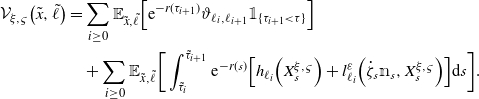
, the process
$(\xi,\varsigma)\in\mathcal{U}^{\varepsilon}\times\mathcal{S}$
, the process ![]() evolves as
evolves as
where
 $\tilde{\tau}_{i}=\tau_{i}\wedge\tau$
and
$\tilde{\tau}_{i}=\tau_{i}\wedge\tau$
and ![]() . Before introducing the corresponding functional cost
. Before introducing the corresponding functional cost
 $\mathcal{V}_{\xi,\varsigma}$
of
$\mathcal{V}_{\xi,\varsigma}$
of
 $(\xi,\varsigma)\in\mathcal{U}^{\varepsilon}\times\mathcal{S}$
, let us define the penalization function
$(\xi,\varsigma)\in\mathcal{U}^{\varepsilon}\times\mathcal{S}$
, let us define the penalization function
 $\psi_{\varepsilon}$
. Consider
$\psi_{\varepsilon}$
. Consider
 $\varphi$
as a function from
$\varphi$
as a function from
 $\mathbb{R}$
to itself that is in
$\mathbb{R}$
to itself that is in
 $\textrm{C}^{\infty}(\mathbb{R})$
and satisfies
$\textrm{C}^{\infty}(\mathbb{R})$
and satisfies
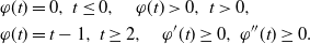 \begin{align}&\varphi(t)=0,\ t\leq0,\quad\varphi(t)>0,\ t>0,\\&\varphi(t)=t-1,\ t\geq2,\quad\varphi^{\prime}(t)\geq0,\ \varphi^{\prime\prime}(t)\geq0.\end{align}
Then,
 $\psi_{\varepsilon}$
is taken as
$\psi_{\varepsilon}$
is taken as
 $\psi_{\varepsilon}(t)=\varphi(t/\varepsilon)$
, for each
$\psi_{\varepsilon}(t)=\varphi(t/\varepsilon)$
, for each
 $\varepsilon\in(0,1)$
. Also, for each
$\varepsilon\in(0,1)$
. Also, for each
 $(x,\ell)\in\overline{\mathcal{O}}\times\mathbb{I}$
fixed, we define the Legendre transform of
$(x,\ell)\in\overline{\mathcal{O}}\times\mathbb{I}$
fixed, we define the Legendre transform of
 $H_{\ell}^{\varepsilon}(\gamma,x)\,:\!=\, H^{\varepsilon}(\gamma,x,\ell)\,:\!=\,\psi_{\varepsilon}\big(|\gamma|^{2}-g_{\ell}(x)^{2}\big)$
by
$H_{\ell}^{\varepsilon}(\gamma,x)\,:\!=\, H^{\varepsilon}(\gamma,x,\ell)\,:\!=\,\psi_{\varepsilon}\big(|\gamma|^{2}-g_{\ell}(x)^{2}\big)$
by
 \begin{equation*}l_{\ell}^{\varepsilon}(y,x)\,:\!=\, l^{\varepsilon}(y,x,\ell)\,:\!=\, \sup_{\gamma\in\mathbb{R}^{d}}\left\{\langle \gamma,y \rangle-H_{\ell}^{\varepsilon}(\gamma,x)\right\},\quad \text{for}\ y\in\mathbb{R}^{d}.\end{equation*}
Notice that, for each
 $(x,\ell)\in\overline{\mathcal{O}}\times\mathbb{I}$
fixed,
$(x,\ell)\in\overline{\mathcal{O}}\times\mathbb{I}$
fixed,
 $H_{\ell}^{\varepsilon}(\gamma,x)$
is a
$H_{\ell}^{\varepsilon}(\gamma,x)$
is a
 $\textrm{C}^{2}$
and convex function with respect to the variable
$\textrm{C}^{2}$
and convex function with respect to the variable
 $\gamma\in\mathbb{R}^{d}$
, since
$\gamma\in\mathbb{R}^{d}$
, since
 $\psi_{\varepsilon}\in \textrm{C}^{\infty}(\mathbb{R})$
is convex. The penalized cost of
$\psi_{\varepsilon}\in \textrm{C}^{\infty}(\mathbb{R})$
is convex. The penalized cost of
 $(\xi,\varsigma)\in\mathcal{U}^{\varepsilon}\times\mathcal{S}$
is defined by
$(\xi,\varsigma)\in\mathcal{U}^{\varepsilon}\times\mathcal{S}$
is defined by
The value function for this problem is given by
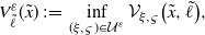 \begin{equation}V_{\tilde{\ell}}^{\varepsilon}(\tilde{x})\,:\!=\,\inf_{(\xi,\varsigma)\in\mathcal{U}^{\varepsilon}}\mathcal{V}_{\xi,\varsigma}\big(\tilde{x},\tilde{\ell}\big),\end{equation}
whose corresponding HJB equation is
 \begin{align}\max\bigg\{[c_{\ell}-\mathcal{L}_{\ell}] u_{\ell}^{\varepsilon}+ \sup_{y\in\mathbb{R}^{d}}\Big\{\Big\langle \textrm{D}^{1}u_{\ell}^{\varepsilon},y\Big\rangle-l_{\ell}^{\varepsilon}(y,\cdot)\Big\}-h_{\ell},u_{\ell}^{\varepsilon}-\mathcal{M}_{\ell}u^{\varepsilon}\bigg\}= 0 ,\ \text{in}\ \mathcal{O},&\\\text{s.t.}\ \ u_{\ell}^{\varepsilon}=0,\ \text{on}\ \partial\mathcal{O}, &\end{align}
where
 $\mathcal{L}_{\ell}, \mathcal{M}_{\ell}$
are as in (2.3), (2.10), respectively. Observe that (2.19) can be rewritten as
$\mathcal{L}_{\ell}, \mathcal{M}_{\ell}$
are as in (2.3), (2.10), respectively. Observe that (2.19) can be rewritten as
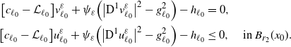
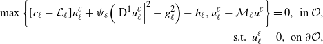 \begin{align}\max\left\{[c_{\ell}-\mathcal{L}_{\ell}] u_{\ell}^{\varepsilon}+\psi_{\varepsilon}\Big(\Big|\textrm{D}^{1}u_{\ell}^{\varepsilon}\Big|^{2}- g_{\ell}^{2}\Big)-h_{\ell},u_{\ell}^{\varepsilon}-\mathcal{M}_{\ell}u^{\varepsilon}\right\}= 0 ,\ \text{in}\ \mathcal{O},&\\\text{s.t.}\ \ u_{\ell}^{\varepsilon}=0,\ \text{on}\ \partial\mathcal{O},&\end{align}
because of
 $H^{\varepsilon}_{\ell}(\gamma,x)=\sup_{y\in\mathbb{R}^{d}}\big\{\langle \gamma,y\rangle-l^{\varepsilon}_{\ell}(y,x)\big\}$
. Under Assumptions (H1)–(H4), the following result is obtained, whose proof is given in the next section; see Subsection 3.1.
$H^{\varepsilon}_{\ell}(\gamma,x)=\sup_{y\in\mathbb{R}^{d}}\big\{\langle \gamma,y\rangle-l^{\varepsilon}_{\ell}(y,x)\big\}$
. Under Assumptions (H1)–(H4), the following result is obtained, whose proof is given in the next section; see Subsection 3.1.
Proposition 2.1. For each
 $\varepsilon\in(0,1)$
fixed, there exists a unique nonnegative strong solution
$\varepsilon\in(0,1)$
fixed, there exists a unique nonnegative strong solution
 $u^{\varepsilon}=\big(u^{\varepsilon}_{1},\dots,u^{\varepsilon}_{m}\big)$
to the HJB equation (2.20) where
$u^{\varepsilon}=\big(u^{\varepsilon}_{1},\dots,u^{\varepsilon}_{m}\big)$
to the HJB equation (2.20) where
 $u^{\varepsilon}_{\ell}\in \textrm{C}^{0,1}\big(\overline{\mathcal{O}}\big)\cap \textrm{W}^{2,\infty}_{\textrm{loc}}(\mathcal{O})$
for each
$u^{\varepsilon}_{\ell}\in \textrm{C}^{0,1}\big(\overline{\mathcal{O}}\big)\cap \textrm{W}^{2,\infty}_{\textrm{loc}}(\mathcal{O})$
for each
 $\ell\in\mathbb{I}$
.
$\ell\in\mathbb{I}$
.
3. Existence and uniqueness of the solution to the HJB equations
This section is devoted to guarantee existence and uniqueness of the solution to the HJB equations (2.9) and (2.20). The solution
 $u^{\varepsilon}$
to (2.20), with
$u^{\varepsilon}$
to (2.20), with
 $\varepsilon\in(0,1)$
fixed, will be constructed as the limit of a sequence of functions
$\varepsilon\in(0,1)$
fixed, will be constructed as the limit of a sequence of functions
 $\big\{u^{\varepsilon,\delta}\big\}_{\delta\in(0,1)}$
, when
$\big\{u^{\varepsilon,\delta}\big\}_{\delta\in(0,1)}$
, when
 $\delta$
goes to zero, which are solutions to the following NPDS:
$\delta$
goes to zero, which are solutions to the following NPDS:
 \begin{align}[c_{\ell}-\mathcal{L}_{\ell}] u_{\ell}^{\varepsilon,\delta}+ \psi_{\varepsilon}\bigg(\Big|\textrm{D}^{1} u_{\ell}^{\varepsilon,\delta}\Big|^{2}- g_{\ell}^{2}\bigg)+\displaystyle\sum_{\kappa\in\mathbb{I}\setminus\{\ell\}}\psi_{\delta}\Big(u_{\ell}^{\varepsilon,\delta}-u_{\kappa}^{\varepsilon,\delta} -\vartheta_{\ell,\kappa}\Big)= h_{\ell} ,\ \text{in}\ \mathcal{O},&\\\text{s.t.}\ \ u^{\varepsilon,\delta}_{\ell}=0,\ \text{on}\ \partial\mathcal{O}.&\end{align}
The Schaefer fixed point theorem is employed to guarantee the existence of the classic solution to
 $u^{\varepsilon,\delta}$
to (3.1). For that aim we need some a priori estimates of
$u^{\varepsilon,\delta}$
to (3.1). For that aim we need some a priori estimates of
 $u^{\varepsilon,\delta}$
, which will also help to verify the theorems seen in the section above.
$u^{\varepsilon,\delta}$
, which will also help to verify the theorems seen in the section above.
Remark 3.1. From now on, we consider cut-off functions
 $\omega\in \textrm{C}^{\infty}_{\textrm{c}}( \mathcal{O})$
which satisfy
$\omega\in \textrm{C}^{\infty}_{\textrm{c}}( \mathcal{O})$
which satisfy
 $0\leq\omega\leq1$
,
$0\leq\omega\leq1$
,
 $\omega=1$
on the open ball
$\omega=1$
on the open ball
 $B_{\beta r}\subset B_{\beta^{\prime}r}\subset\mathcal{O}$
and
$B_{\beta r}\subset B_{\beta^{\prime}r}\subset\mathcal{O}$
and
 $\omega=0$
on
$\omega=0$
on
 $\mathcal{O} \setminus B_{\beta^{\prime} r}$
, with
$\mathcal{O} \setminus B_{\beta^{\prime} r}$
, with
 $r>0$
,
$r>0$
,
 $\beta^{\prime}= \frac{\beta+1}{2}$
, and
$\beta^{\prime}= \frac{\beta+1}{2}$
, and
 $\beta\in(0,1]$
. It is also assumed that
$\beta\in(0,1]$
. It is also assumed that
 $||\omega||_{\textrm{C}^{2}\big(\overline{B}_{\beta r}\big)}\leq K_{1}$
, where
$||\omega||_{\textrm{C}^{2}\big(\overline{B}_{\beta r}\big)}\leq K_{1}$
, where
 $K_{1}>0$
is a constant independent of
$K_{1}>0$
is a constant independent of
 $\varepsilon$
and
$\varepsilon$
and
 $\delta$
.
$\delta$
.
Under Assumptions (H1)–(H4), the following results are obtained. Their proofs can be found in the appendix.
Lemma 3.1. Let
 $ u^{\varepsilon,\delta}=\Big(u_{1}^{\varepsilon,\delta},\dots,u_{m}^{\varepsilon,\delta}\Big)$
be a vector solution to the NPDS (3.1), whose components are in
$ u^{\varepsilon,\delta}=\Big(u_{1}^{\varepsilon,\delta},\dots,u_{m}^{\varepsilon,\delta}\Big)$
be a vector solution to the NPDS (3.1), whose components are in
 $\textrm{C}^{4}\big(\overline{\mathcal{O}}\big) $
. Then, for each
$\textrm{C}^{4}\big(\overline{\mathcal{O}}\big) $
. Then, for each
 $\ell\in\mathbb{I}$
, there exist positive constants
$\ell\in\mathbb{I}$
, there exist positive constants
 $C_{1},C_{2},C_{3}$
independent of
$C_{1},C_{2},C_{3}$
independent of
 $\varepsilon,\delta$
such that if
$\varepsilon,\delta$
such that if
 $x\in\overline{\mathcal{O}}$
, then
$x\in\overline{\mathcal{O}}$
, then
 \begin{align} &0\leq u_{\ell}^{\varepsilon,\delta}(x)\leq C_{1},\end{align}
 \begin{align} &\Big|\textrm{D}^{1}u_{\ell}^{\varepsilon,\delta}(x)\Big|\leq C_{2},\end{align}
 \begin{align} &\omega(x)\Big|\textrm{D}^{2}u_{\ell}^{\varepsilon,\delta}(x)\Big|\leq C_{3}. \end{align}
Proposition 3.1. Let
 $\varepsilon,\delta\in(0,1)$
be fixed. There exists a unique nonnegative solution
$\varepsilon,\delta\in(0,1)$
be fixed. There exists a unique nonnegative solution
 $u^{\varepsilon,\delta}=\big(u^{\varepsilon,\delta}_{1},\dots,u^{\varepsilon,\delta}_{m}\big)$
to the NPDS (3.1) where
$u^{\varepsilon,\delta}=\big(u^{\varepsilon,\delta}_{1},\dots,u^{\varepsilon,\delta}_{m}\big)$
to the NPDS (3.1) where
 $u^{\varepsilon,\delta}_{\ell}\in \textrm{C}^{4,\alpha^{\prime}}\big(\overline{\mathcal{O}}\big)$
for each
$u^{\varepsilon,\delta}_{\ell}\in \textrm{C}^{4,\alpha^{\prime}}\big(\overline{\mathcal{O}}\big)$
for each
 $\ell\in\mathbb{I}$
.
$\ell\in\mathbb{I}$
.
Remark 3.2. The NPDS (3.1) has been studied in a number of similar problems. One of them is when the second term on the left-hand side of (3.1) does not appear. This equation was considered by Lenhart and Belbas [Reference Lenhart and Belbas13] to study a HJB equation related to a switching stochastic control problem when there is no loop of zero cost. Later, Yamada [Reference Yamada18] used an NPDS similar to (3.1) to study the HJB equation (2.12). Equations of this type also appear in some stochastic singular control problems; see [Reference Kelbert and Moreno-Franco12] and the references therein.
3.1. Proof of Proposition 2.1
Let
 $\varepsilon\in(0,1)$
and
$\varepsilon\in(0,1)$
and
 $\ell\in\mathbb{I}$
be fixed. Since
$\ell\in\mathbb{I}$
be fixed. Since
 $u^{\varepsilon,\delta}_{\ell}, \ \partial_{ij}u^{\varepsilon,\delta}_{\ell}$
are bounded, uniformly in
$u^{\varepsilon,\delta}_{\ell}, \ \partial_{ij}u^{\varepsilon,\delta}_{\ell}$
are bounded, uniformly in
 $\delta$
, on the spaces
$\delta$
, on the spaces
 $\Big(\text{C}^{1}\big(\overline{\mathcal{O}}\big),||{\cdot}||_{\text{C}^{1}(\mathcal{O})}\Big)$
and
$\Big(\text{C}^{1}\big(\overline{\mathcal{O}}\big),||{\cdot}||_{\text{C}^{1}(\mathcal{O})}\Big)$
and
 $\Big(\text{C}\big(\overline{B}_{ r}\big),||{\cdot}||_{\text{C}(B_{ r})}\Big)$
, respectively, where
$\Big(\text{C}\big(\overline{B}_{ r}\big),||{\cdot}||_{\text{C}(B_{ r})}\Big)$
, respectively, where
 $B_{r}\subset\mathcal{O}$
(see Lemma 3.1), and using the Arzelà–Ascoli compactness criterion (see [Reference Evans8, p. 718]) and the fact that for each
$B_{r}\subset\mathcal{O}$
(see Lemma 3.1), and using the Arzelà–Ascoli compactness criterion (see [Reference Evans8, p. 718]) and the fact that for each
 $p\in(1,\infty)$
,
$p\in(1,\infty)$
,
 $\Big(\textrm{L}^{p}\big(B_{\beta r}\big),||{\cdot}||_{\textrm{L}^{p}(B_{r})}\Big)$
, with
$\Big(\textrm{L}^{p}\big(B_{\beta r}\big),||{\cdot}||_{\textrm{L}^{p}(B_{r})}\Big)$
, with
 $B_{r}\subset\mathcal{O}$
, is a reflexive space (see [Reference Adams and Fournier1, Theorem 2.46, p. 49]), it can be proven that there exist a subsequence
$B_{r}\subset\mathcal{O}$
, is a reflexive space (see [Reference Adams and Fournier1, Theorem 2.46, p. 49]), it can be proven that there exist a subsequence
 $\Big\{u^{\varepsilon,\delta_{\hat{n}}}_{\ell}\Big\}_{\hat{n}\geq1}$
of
$\Big\{u^{\varepsilon,\delta_{\hat{n}}}_{\ell}\Big\}_{\hat{n}\geq1}$
of
 $\big\{u^{\varepsilon,\delta}_{\ell}\big\}_{\delta\in(0,1)}$
and a function
$\big\{u^{\varepsilon,\delta}_{\ell}\big\}_{\delta\in(0,1)}$
and a function
 $u^{\varepsilon}_{\ell}$
in
$u^{\varepsilon}_{\ell}$
in
 $\textrm{C}^{0,1}\big(\overline{\mathcal{O}}\big)\cap \textrm{W}^{2,\infty}_{\textrm{loc}}(\mathcal{O})$
such that
$\textrm{C}^{0,1}\big(\overline{\mathcal{O}}\big)\cap \textrm{W}^{2,\infty}_{\textrm{loc}}(\mathcal{O})$
such that
 \begin{align}&\text{$u^{\varepsilon,\delta_{\hat{n}}}_{\ell}\underset{\delta_{\hat{n}}\rightarrow0}{\longrightarrow}u^{\varepsilon}_{\ell}$ in $\textrm{C}\big(\overline{\mathcal{O}}\big)$, $\partial_{i}u^{\varepsilon,\delta_{\hat{n}}}_{\ell}\underset{\delta_{\hat{n}}\rightarrow0}{\longrightarrow}\partial_{i} u^{\varepsilon}_{\ell}$ $\text{in}\ \text{C}_{\textrm{loc}}(\mathcal{O})$,}\\ &\text{$\partial_{ij}u^{\varepsilon,\delta_{\hat{n}}}_{\ell}\underset{\delta_{\hat{n}}\rightarrow0}{\longrightarrow}\partial_{ij}u^{\varepsilon}_{\ell}$, weakly $ \textrm{L}^{p}_{\textrm{loc}}(\mathcal{O})$, for each $p\in(1,\infty)$.}\end{align}
We proceed to proving Proposition 2.1.
Proof of Proposition 2.1. Existence. Taking
 $\kappa\in\mathbb{I}\setminus\{\ell\}$
, and using (2.3), (3.1), and Lemma 3.1, we have that
$\kappa\in\mathbb{I}\setminus\{\ell\}$
, and using (2.3), (3.1), and Lemma 3.1, we have that
 $\psi_{\delta}\Big(u^{\varepsilon,\delta}_{\ell}-u^{\varepsilon,\delta}_{\kappa} -\vartheta_{\ell,\kappa}\Big)$
is locally bounded, uniformly in
$\psi_{\delta}\Big(u^{\varepsilon,\delta}_{\ell}-u^{\varepsilon,\delta}_{\kappa} -\vartheta_{\ell,\kappa}\Big)$
is locally bounded, uniformly in
 $\delta$
. From here and (3.5), we obtain that
$\delta$
. From here and (3.5), we obtain that
 $u^{\varepsilon}_{\ell}-u^{\varepsilon}_{\kappa} -\vartheta_{\ell,\kappa}\leq0$
in
$u^{\varepsilon}_{\ell}-u^{\varepsilon}_{\kappa} -\vartheta_{\ell,\kappa}\leq0$
in
 $\mathcal{O}$
. Then,
$\mathcal{O}$
. Then,
 \begin{equation} u^{\varepsilon}_{\ell}-\mathcal{M}_{\ell}u^{\varepsilon}\leq0,\quad \text{in}\ \mathcal{O}. \end{equation}
Note that the previous inequality is true on the boundary set
 $\partial\mathcal{O}$
, since
$\partial\mathcal{O}$
, since
 $u^{\varepsilon,\delta}_{\ell}=u^{\varepsilon,\delta}_{\kappa}=0$
on
$u^{\varepsilon,\delta}_{\ell}=u^{\varepsilon,\delta}_{\kappa}=0$
on
 $\partial\mathcal{O}$
and
$\partial\mathcal{O}$
and
 $\vartheta_{\ell,\kappa}\geq0$
. Recall that the operator
$\vartheta_{\ell,\kappa}\geq0$
. Recall that the operator
 $\mathcal{M}_{\ell}$
is defined in (2.10). On the other hand, since
$\mathcal{M}_{\ell}$
is defined in (2.10). On the other hand, since
 $u^{\varepsilon,\delta_{\hat{n}}}_{\ell}$
is the unique solution to (3.1), when
$u^{\varepsilon,\delta_{\hat{n}}}_{\ell}$
is the unique solution to (3.1), when
 $\delta=\delta_{\hat{n}}$
, it follows that
$\delta=\delta_{\hat{n}}$
, it follows that
 \begin{equation} \int_{B_{r}}\bigg\{[c_{\ell}-\mathcal{L}_{\ell}] u_{\ell}^{\varepsilon,\delta_{\hat{n}}}+ \psi_{\varepsilon}\Big(\Big|\textrm{D}^{1} u_{\ell}^{\varepsilon,\delta_{\hat{n}}}\Big|^{2}- g_{\ell}^{2}\Big)\bigg\}\varpi\textrm{d} x\leq \int_{B_{r}}h_{\ell}\varpi\textrm{d} x ,\quad\text{for}\ \varpi\in\mathcal{B}(B_{r}), \end{equation}
where
 \begin{equation} \mathcal{B}(A)\,:\!=\,\big\{\varpi\in \text{C}^{\infty}_{\text{c}}(A)\,:\, \varpi\geq0\ \text{and}\ \text{supp}[\varpi]\subset A\subset\mathcal{O} \big\}. \end{equation}
By (3.5) and letting
 $\delta_{\hat{n}}\rightarrow0$
in (3.7), we obtain that
$\delta_{\hat{n}}\rightarrow0$
in (3.7), we obtain that
 \begin{equation} [c_{\ell}-\mathcal{L}_{\ell}] u_{\ell}^{\varepsilon}+ \psi_{\varepsilon}\Big(\Big|\textrm{D}^{1} u_{\ell}^{\varepsilon}\Big|^{2}- g_{\ell}^{2}\Big)\leq h_{\ell}\quad \text{a.e.}\ \text{in} \, \mathcal{O}. \end{equation}
From (3.6) and (3.9),
 $\max\Big\{[c_{\ell}-\mathcal{L}_{\ell}] u_{\ell}^{\varepsilon}+\psi_{\varepsilon}\Big(\Big|\textrm{D}^{1} u_{\ell}^{\varepsilon}\Big|^{2}- g_{\ell}^{2}\Big)-h_{\ell},u^{\varepsilon}_{\ell}-\mathcal{M}_{\ell}u^{\varepsilon}\Big\}\leq 0$
a.e. in
$\max\Big\{[c_{\ell}-\mathcal{L}_{\ell}] u_{\ell}^{\varepsilon}+\psi_{\varepsilon}\Big(\Big|\textrm{D}^{1} u_{\ell}^{\varepsilon}\Big|^{2}- g_{\ell}^{2}\Big)-h_{\ell},u^{\varepsilon}_{\ell}-\mathcal{M}_{\ell}u^{\varepsilon}\Big\}\leq 0$
a.e. in
 $\mathcal{O}$
. We shall prove that if
$\mathcal{O}$
. We shall prove that if
 \begin{equation} u^{\varepsilon}_{\ell}(x^{*})-\mathcal{M}_{\ell}u^{\varepsilon}(x^{*})<0,\quad \text{for some}\ x^{*}\in\mathcal{O}, \end{equation}
then there exists a neighborhood
 $\mathcal{N}_{x^{*}}\subset\mathcal{O}$
of
$\mathcal{N}_{x^{*}}\subset\mathcal{O}$
of
 $x^{*}$
such that
$x^{*}$
such that
 \begin{equation} [c_{\ell}-\mathcal{L}_{\ell}] u_{\ell}^{\varepsilon}+\psi_{\varepsilon}\Big(\Big|\textrm{D}^{1} u_{\ell}^{\varepsilon}\Big|^{2}- g_{\ell}^{2}\Big)= h_{\ell},\quad \text{a.e.}\ \text{in} \, \mathcal{N}_{x^{*}}. \end{equation}
Assume (3.10) holds. Then, taking
 $\kappa\in\mathbb{I}\setminus\{\ell\}$
, we see that
$\kappa\in\mathbb{I}\setminus\{\ell\}$
, we see that
 $u^{\varepsilon}_{\ell}-u^{\varepsilon}_{\kappa} -\vartheta_{\ell,\kappa}\leq u^{\varepsilon}_{\ell}-\mathcal{M}_{\ell}u^{\varepsilon}<0$
at
$u^{\varepsilon}_{\ell}-u^{\varepsilon}_{\kappa} -\vartheta_{\ell,\kappa}\leq u^{\varepsilon}_{\ell}-\mathcal{M}_{\ell}u^{\varepsilon}<0$
at
 $x^{*}$
. Since
$x^{*}$
. Since
 $u^{\varepsilon}_{\ell}-u^{\varepsilon}_{\kappa} $
is a continuous function, there exists a ball
$u^{\varepsilon}_{\ell}-u^{\varepsilon}_{\kappa} $
is a continuous function, there exists a ball
 $B_{r_{\kappa}}\subset\mathcal{O}$
such that
$B_{r_{\kappa}}\subset\mathcal{O}$
such that
 $x^{*}\in B_{r_{\kappa}}$
and
$x^{*}\in B_{r_{\kappa}}$
and
 $u^{\varepsilon}_{\ell}-u^{\varepsilon}_{\kappa} -\vartheta_{\ell,\kappa}<0$
in
$u^{\varepsilon}_{\ell}-u^{\varepsilon}_{\kappa} -\vartheta_{\ell,\kappa}<0$
in
 $B_{r_{\kappa}}$
. From here, and defining
$B_{r_{\kappa}}$
. From here, and defining
 $\mathcal{N}_{x^{*}}$
as
$\mathcal{N}_{x^{*}}$
as
 $\bigcap_{\kappa\in\mathbb{I}\setminus\{\ell\}}B_{r_{\kappa}}$
, we have that
$\bigcap_{\kappa\in\mathbb{I}\setminus\{\ell\}}B_{r_{\kappa}}$
, we have that
 $\mathcal{N}_{x^{*}}\subset\mathcal{O}$
is a neighborhood of
$\mathcal{N}_{x^{*}}\subset\mathcal{O}$
is a neighborhood of
 $x^{*}$
and
$x^{*}$
and
 \begin{equation} u^{\varepsilon}_{\ell}-u^{\varepsilon}_{\kappa} -\vartheta_{\ell,\kappa}<0,\quad \text{ in}\ \mathcal{N}_{x^{*}},\ \text{for}\ \kappa\in\mathbb{I}\setminus\{\ell\}. \end{equation}
Meanwhile, observe that
 \begin{equation} \Big|\Big|u^{\varepsilon,\delta_{\hat{n}}}_{\ell}-u^{\varepsilon,\delta_{\hat{n}}}_{\kappa} -\big(u^{\varepsilon}_{\ell}-u^{\varepsilon}_{\kappa} \big)\Big|\Big|_{\text{C}(\mathcal{O})}\underset{\delta_{\hat{n}}\rightarrow0}{\longrightarrow}0,\quad\text{for}\ \kappa\in\mathbb{I}\setminus\{\ell\}, \end{equation}
since (3.5) holds. Then, by (3.12)–(3.13), we have that for each
 $\kappa\in\mathbb{I}\setminus\{\ell\}$
, there exists a
$\kappa\in\mathbb{I}\setminus\{\ell\}$
, there exists a
 $\delta^{(\kappa)}\in(0,1)$
such that if
$\delta^{(\kappa)}\in(0,1)$
such that if
 $\delta_{\hat{n}}\leq\delta^{(\kappa)}$
, then
$\delta_{\hat{n}}\leq\delta^{(\kappa)}$
, then
 $u^{\varepsilon,\delta_{\hat{n}}}_{\ell}-u^{\varepsilon,\delta_{\hat{n}}}_{\kappa} -\vartheta_{\ell,\kappa}<0$
in
$u^{\varepsilon,\delta_{\hat{n}}}_{\ell}-u^{\varepsilon,\delta_{\hat{n}}}_{\kappa} -\vartheta_{\ell,\kappa}<0$
in
 $\mathcal{N}_{x^{*}}$
. Taking
$\mathcal{N}_{x^{*}}$
. Taking
 $\delta^{\prime}\,:\!=\,\min_{\kappa\in\mathbb{I}\setminus\{\ell\}}\{\delta^{(\kappa)}\}$
, it follows that
$\delta^{\prime}\,:\!=\,\min_{\kappa\in\mathbb{I}\setminus\{\ell\}}\{\delta^{(\kappa)}\}$
, it follows that
 $u^{\varepsilon,\delta_{\hat{n}}}_{\ell}-u^{\varepsilon,\delta_{\hat{n}}}_{\kappa} -\vartheta_{\ell,\kappa}<0$
in
$u^{\varepsilon,\delta_{\hat{n}}}_{\ell}-u^{\varepsilon,\delta_{\hat{n}}}_{\kappa} -\vartheta_{\ell,\kappa}<0$
in
 $\mathcal{N}_{x^{*}}$
, for all
$\mathcal{N}_{x^{*}}$
, for all
 $\delta_{\hat{n}}\leq\delta^{\prime}$
and
$\delta_{\hat{n}}\leq\delta^{\prime}$
and
 $\kappa\in\mathbb{I}\setminus\{\ell\}$
. From here and since for each
$\kappa\in\mathbb{I}\setminus\{\ell\}$
. From here and since for each
 $\delta_{\hat{n}}\leq\delta^{\prime}$
,
$\delta_{\hat{n}}\leq\delta^{\prime}$
,
 $u^{\varepsilon,\delta_{\hat{n}}}_{\ell}$
is the unique solution to (3.1), when
$u^{\varepsilon,\delta_{\hat{n}}}_{\ell}$
is the unique solution to (3.1), when
 $\delta=\delta_{\hat{n}}$
, this implies that
$\delta=\delta_{\hat{n}}$
, this implies that
 \begin{equation*} \int_{\mathcal{N}_{x^{*}}}\Big\{[c_{\ell}-\mathcal{L}_{\ell}] u_{\ell}^{\varepsilon,\delta_{\hat{n}}}+ \psi_{\varepsilon}\Big(\Big|\textrm{D}^{1} u_{\ell}^{\varepsilon,\delta_{\hat{n}}}\Big|^{2}- g_{\ell}^{2}\Big)\Big\}\varpi\textrm{d} x= \int_{\mathcal{N}_{x^{*}}}h_{\ell}\varpi\textrm{d} x, \quad\text{for}\ \varpi\in\mathcal{B}(\mathcal{N}_{x^{*}}). \end{equation*}
Therefore, (3.11) holds. Hence, we get that for each
 $\varepsilon\in(0,1)$
,
$\varepsilon\in(0,1)$
,
 $u^{\varepsilon}=\big(u^{\varepsilon}_{1},\dots,u^{\varepsilon}_{m}\big)$
is a solution to the HJB equation (2.19).
$u^{\varepsilon}=\big(u^{\varepsilon}_{1},\dots,u^{\varepsilon}_{m}\big)$
is a solution to the HJB equation (2.19).
Proof of Proposition 2.1. Uniqueness. Let
 $\varepsilon\in(0,1)$
be fixed. Suppose that
$\varepsilon\in(0,1)$
be fixed. Suppose that
 $u^{\varepsilon}=\big(u^{\varepsilon}_{1},\dots,u^{\varepsilon}_{m}\big)$
and
$u^{\varepsilon}=\big(u^{\varepsilon}_{1},\dots,u^{\varepsilon}_{m}\big)$
and
 $v^{\varepsilon}=\big(v^{\varepsilon}_{1},\dots,v^{\varepsilon}_{m}\big)$
are two solutions to the HJB equation (2.20) whose components belong to
$v^{\varepsilon}=\big(v^{\varepsilon}_{1},\dots,v^{\varepsilon}_{m}\big)$
are two solutions to the HJB equation (2.20) whose components belong to
 $\textrm{C}^{0,1}\big(\overline{\mathcal{O}}\big)\cap \textrm{W}^{2,\infty}_{\textrm{loc}}(\mathcal{O})$
. Take
$\textrm{C}^{0,1}\big(\overline{\mathcal{O}}\big)\cap \textrm{W}^{2,\infty}_{\textrm{loc}}(\mathcal{O})$
. Take
 $(x_{0},\ell_{0})\in\overline{\mathcal{O}}\times\mathbb{I}$
such that
$(x_{0},\ell_{0})\in\overline{\mathcal{O}}\times\mathbb{I}$
such that
 \begin{equation} u^{\varepsilon}_{\ell_{0}}(x_{0})-v^{\varepsilon}_{\ell_{0}}(x_{0})=\sup_{(x,\ell)\in\overline{\mathcal{O}}\times\mathbb{I}}\big\{u^{\varepsilon}_{\ell}(x)-v_{\ell}^{\varepsilon}(x)\big\}. \end{equation}
Notice that by (3.14), we only need to verify that
 \begin{equation} u^{\varepsilon}_{\ell_{0}}(x_{0})-v^{\varepsilon}_{\ell_{0}}(x_{0})\leq0, \end{equation}
which is trivially true if
 $x_{0}\in\partial\mathcal{O}$
, since
$x_{0}\in\partial\mathcal{O}$
, since
 $u^{\varepsilon}_{\ell_{0}}-v^{\varepsilon}_{\ell_{0}}=0$
on
$u^{\varepsilon}_{\ell_{0}}-v^{\varepsilon}_{\ell_{0}}=0$
on
 $\partial\mathcal{O}$
. Let us assume
$\partial\mathcal{O}$
. Let us assume
 $x_{0}\in\mathcal{O}$
. We shall verify (3.15) by contradiction. Suppose that
$x_{0}\in\mathcal{O}$
. We shall verify (3.15) by contradiction. Suppose that
 $u^{\varepsilon}_{\ell_{0}}-v^{\varepsilon}_{\ell_{0}}>0$
at
$u^{\varepsilon}_{\ell_{0}}-v^{\varepsilon}_{\ell_{0}}>0$
at
 $x_{0}$
. Then, by continuity of
$x_{0}$
. Then, by continuity of
 $u^{\varepsilon}_{\ell_{0}}-v^{\varepsilon}_{\ell_{0}}$
, there exists a ball
$u^{\varepsilon}_{\ell_{0}}-v^{\varepsilon}_{\ell_{0}}$
, there exists a ball
 $B_{r_{1}}(x_{0})\subset\mathcal{O}$
such that
$B_{r_{1}}(x_{0})\subset\mathcal{O}$
such that
 \begin{equation} c_{\ell_{0}}\Big[u^{\varepsilon}_{\ell_{0}}-v^{\varepsilon}_{\ell_{0}}\Big]\geq\min_{x\in B_{r_{1}}(x_{0})}\Big\{c_{\ell_{0}}(x)\Big[u^{\varepsilon}_{\ell_{0}}(x)-v^{\varepsilon}_{\ell_{0}}(x)\Big]\Big\}>0,\quad \text{in}\ B_{r_{1}}(x_{0}). \end{equation}
The last inequality is true because of
 $c_{\ell_{0}}>0$
in
$c_{\ell_{0}}>0$
in
 $\mathcal{O}$
. Taking
$\mathcal{O}$
. Taking
 $\ell_{1}\in\mathbb{I}$
such that
$\ell_{1}\in\mathbb{I}$
such that
 \begin{equation} \mathcal{M}_{\ell_{0}}v^{\varepsilon}(x_{0})=v^{\varepsilon}_{\ell_{1}}(x_{0} )+\vartheta_{\ell_{0},\ell_{1}}, \end{equation}
by (2.20) and (3.14), we get that
 $v^{\varepsilon}_{\ell_{0}}-\big(v^{\varepsilon}_{\ell_{1}}+\vartheta_{\ell_{0},\ell_{1}}\big) =v^{\varepsilon}_{\ell_{0}}-\mathcal{M}_{\ell_{0}}v^{\varepsilon}\leq u^{\varepsilon}_{\ell_{0}}-\mathcal{M}_{\ell_{0}}u^{\varepsilon}\leq 0$
at
$v^{\varepsilon}_{\ell_{0}}-\big(v^{\varepsilon}_{\ell_{1}}+\vartheta_{\ell_{0},\ell_{1}}\big) =v^{\varepsilon}_{\ell_{0}}-\mathcal{M}_{\ell_{0}}v^{\varepsilon}\leq u^{\varepsilon}_{\ell_{0}}-\mathcal{M}_{\ell_{0}}u^{\varepsilon}\leq 0$
at
 $x_{0}$
. If
$x_{0}$
. If
 $v^{\varepsilon}_{\ell_{0}}(x_{0})-\mathcal{M}_{\ell_{0}}v^{\varepsilon}(x_{0})<0$
, there exists a ball
$v^{\varepsilon}_{\ell_{0}}(x_{0})-\mathcal{M}_{\ell_{0}}v^{\varepsilon}(x_{0})<0$
, there exists a ball
 $B_{r_{2}}(x_{0})\subset\mathcal{O}$
such that
$B_{r_{2}}(x_{0})\subset\mathcal{O}$
such that
 $v^{\varepsilon}_{\ell_{0}}-\mathcal{M}_{\ell_{0}}v^{\varepsilon}<0$
in
$v^{\varepsilon}_{\ell_{0}}-\mathcal{M}_{\ell_{0}}v^{\varepsilon}<0$
in
 $B_{r_{2}}(x_{0})$
. Moreover, from (2.20),
$B_{r_{2}}(x_{0})$
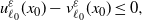
. Moreover, from (2.20),
 \begin{align} \big[c_{\ell_{0}}-\mathcal{L}_{\ell_{0}}\big] v_{\ell_{0}}^{\varepsilon}+\psi_{\varepsilon}\Big(\big|\textrm{D}^{1} v_{\ell_{0}}^{\varepsilon}\big|^{2}- g_{\ell_{0}}^{2}\Big)-h_{\ell_{0}}&=0,\\ \big[c_{\ell_{0}}-\mathcal{L}_{\ell_{0}}\big] u_{\ell_{0}}^{\varepsilon}+\psi_{\varepsilon}\Big(\big|\textrm{D}^{1} u_{\ell_{0}}^{\varepsilon}\big|^{2}- g_{\ell_{0}}^{2}\Big)-h_{\ell_{0}}&\leq0, \quad\text{in}\ B_{r_{2}}(x_{0}). \end{align}
Notice that
 $\psi_{\varepsilon}\Big(\Big|\textrm{D}^{1} u_{\ell_{0}}^{\varepsilon}\Big|^{2}- g_{\ell_{0}}^{2}\Big)-\psi_{\varepsilon}\Big(\Big|\textrm{D}^{1} v_{\ell_{0}}^{\varepsilon}\Big|^{2}- g_{\ell_{0}}^{2}\Big)$
is a continuous function in
$\psi_{\varepsilon}\Big(\Big|\textrm{D}^{1} u_{\ell_{0}}^{\varepsilon}\Big|^{2}- g_{\ell_{0}}^{2}\Big)-\psi_{\varepsilon}\Big(\Big|\textrm{D}^{1} v_{\ell_{0}}^{\varepsilon}\Big|^{2}- g_{\ell_{0}}^{2}\Big)$
is a continuous function in
 $\mathcal{O}$
, since
$\mathcal{O}$
, since
 $\partial_{i}u^{\varepsilon}_{\ell_{0}},\partial_{i}v^{\varepsilon}_{\ell_{0}}\in \text{C}^{0}(\mathcal{O})$
, which satisfies
$\partial_{i}u^{\varepsilon}_{\ell_{0}},\partial_{i}v^{\varepsilon}_{\ell_{0}}\in \text{C}^{0}(\mathcal{O})$
, which satisfies
 $\psi_{\varepsilon}\Big(\Big|\textrm{D}^{1} u_{\ell_{0}}^{\varepsilon}\Big|^{2}- g_{\ell_{0}}^{2}\Big)-\psi_{\varepsilon}\Big(\Big|\textrm{D}^{1} v_{\ell_{0}}^{\varepsilon}\Big|^{2}- g_{\ell_{0}}^{2}\Big)=0$
at
$\psi_{\varepsilon}\Big(\Big|\textrm{D}^{1} u_{\ell_{0}}^{\varepsilon}\Big|^{2}- g_{\ell_{0}}^{2}\Big)-\psi_{\varepsilon}\Big(\Big|\textrm{D}^{1} v_{\ell_{0}}^{\varepsilon}\Big|^{2}- g_{\ell_{0}}^{2}\Big)=0$
at
 $x_{0}$
, since
$x_{0}$
, since
 $x_{0}$
is the point where
$x_{0}$
is the point where
 $u^{\varepsilon}_{\ell_{0}}-v^{\varepsilon}_{\ell_{0}}$
attains its maximum. Meanwhile, by Bony’s maximum principle (see [Reference Lions14]), it is known that for every
$u^{\varepsilon}_{\ell_{0}}-v^{\varepsilon}_{\ell_{0}}$
attains its maximum. Meanwhile, by Bony’s maximum principle (see [Reference Lions14]), it is known that for every
 $r\leq r_{3}$
, with
$r\leq r_{3}$
, with
 $r_{3}>0$
small enough,
$r_{3}>0$
small enough,
 \begin{equation} \textrm{tr}\big[a_{\ell_{0}}\textrm{D}^{2}\big[u^{\varepsilon}_{\ell_{0}}-v^{\varepsilon}_{\ell_{0}}\big]\big]\leq0, \quad\text{a.e.}\ \text{in}\ B_{r}(x_{0}). \end{equation}
So, from (3.16), (3.18), and (3.19), we have that for every
 $r\leq \hat{r}\,:\!=\,\min\{r_{1},r_{2},r_{3}\}$
,
$r\leq \hat{r}\,:\!=\,\min\{r_{1},r_{2},r_{3}\}$
,
 \begin{align*} 0&\geq \textrm{tr}\big[a_{\ell_{0}}\textrm{D}^{2}\big[u^{\varepsilon}_{\ell_{0}}-v^{\varepsilon}_{\ell_{0}}\big]\big]\notag\\ &\geq c_{\ell_{0}}\big[u^{\varepsilon}_{\ell_{0}}-v^{\varepsilon}_{\ell_{0}}\big]+\big\langle b_{\ell_{0}},\textrm{D}^{1}\big[u^{\varepsilon}_{\ell_{0}}-v^{\varepsilon}_{\ell_{0}}\big]\big\rangle+\psi_{\varepsilon}\Big(\Big|\textrm{D}^{1} u_{\ell_{0}}^{\varepsilon}\Big|^{2}- g_{\ell_{0}}^{2}\Big)-\psi_{\varepsilon}\Big(\Big|\textrm{D}^{1} v_{\ell_{0}}^{\varepsilon}\Big|^{2}- g_{\ell_{0}}^{2}\Big)\notag\\ &\geq \min_{x\in B_{r_{1}}(x_{0})}\Big\{c_{\ell_{0}}(x)\Big[u^{\varepsilon}_{\ell_{0}}(x)-v^{\varepsilon}_{\ell_{0}}(x)\Big]\Big\} +\big\langle b_{\ell_{0}},\textrm{D}^{1}\big[u^{\varepsilon}_{\ell_{0}}-v^{\varepsilon}_{\ell_{0}}\big]\big\rangle\notag\\ &\quad+\psi_{\varepsilon}\Big(\Big|\textrm{D}^{1} u_{\ell_{0}}^{\varepsilon}\Big|^{2}- g_{\ell_{0}}^{2}\Big)-\psi_{\varepsilon}\Big(\Big|\textrm{D}^{1} v_{\ell_{0}}^{\varepsilon}\Big|^{2}- g_{\ell_{0}}^{2}\Big),\quad\text{a.e.}\ \text{in} \, B_{r}(x_{0}). \end{align*}
Then,
 \begin{align}\lim_{r\rightarrow0}\bigg\{\mathop{\textrm{inf} \,\textrm{ess}}\limits_{B_{r}(x_{0})}\bigg[\psi_{\varepsilon}\Big(\Big|\textrm{D}^{1} u_{\ell_{0}}^{\varepsilon}\Big|^{2}- g_{\ell_{0}}^{2}\Big) & -\psi_{\varepsilon}\Big(\Big|\textrm{D}^{1} v_{\ell_{0}}^{\varepsilon}\Big|^{2}- g_{\ell_{0}}^{2}\Big)\bigg]\bigg\}\nonumber\\& <-\min_{x\in B_{r_{1}}(x_{0})}\Big\{c_{\ell_{0}}(x)\Big[u^{\varepsilon}_{\ell_{0}}(x)-v^{\varepsilon}_{\ell_{0}}(x)\Big]\Big\}<0.\end{align}
This means
 $\psi_{\varepsilon}\Big(\Big|\textrm{D}^{1} u_{\ell_{0}}^{\varepsilon}\Big|^{2}- g_{\ell_{0}}^{2}\Big)-\psi_{\varepsilon}\Big(\Big|\textrm{D}^{1} v_{\ell_{0}}^{\varepsilon}\Big|^{2}- g_{\ell_{0}}^{2}\Big)$
is not continuous at
$\psi_{\varepsilon}\Big(\Big|\textrm{D}^{1} u_{\ell_{0}}^{\varepsilon}\Big|^{2}- g_{\ell_{0}}^{2}\Big)-\psi_{\varepsilon}\Big(\Big|\textrm{D}^{1} v_{\ell_{0}}^{\varepsilon}\Big|^{2}- g_{\ell_{0}}^{2}\Big)$
is not continuous at
 $x_{0}$
which is a contradiction. Thus,
$x_{0}$
which is a contradiction. Thus,
 \begin{equation} 0=v^{\varepsilon}_{\ell_{0}}-\big(v^{\varepsilon}_{\ell_{1}}+\vartheta_{\ell_{0},\ell_{1}}\big) =v^{\varepsilon}_{\ell_{0}}-\mathcal{M}_{\ell_{0}}v^{\varepsilon}\leq u^{\varepsilon}_{\ell_{0}}-\mathcal{M}_{\ell_{0}}u^{\varepsilon}\leq 0\quad\text{at}\ x_{0}. \end{equation}
This implies that
 \begin{align} u^{\varepsilon}_{\ell_{1}}({x_{0} }) & -v^{\varepsilon}_{\ell_{1}}({x_{0} })\geq u^{\varepsilon}_{\ell_{0}}(x_{0})-v^{\varepsilon}_{\ell_{0}}(x_{0})>0,\\v^{\varepsilon}_{\ell_{0}}(x_{0}) & =v^{\varepsilon}_{\ell_{1}}({x_{0} })+\vartheta_{\ell_{0},\ell_{1}}.\nonumber \end{align}
By (3.14) and (3.22), we have that
 $u^{\varepsilon}_{\ell_{1}}-v^{\varepsilon}_{\ell_{1}}$
attains its maximum at
$u^{\varepsilon}_{\ell_{1}}-v^{\varepsilon}_{\ell_{1}}$
attains its maximum at
 $ x_{0} \in\mathcal{O}$
, where its value agrees with
$ x_{0} \in\mathcal{O}$
, where its value agrees with
 $u^{\varepsilon}_{\ell_{0}}(x_{0})-v^{\varepsilon}_{\ell_{0}}(x_{0})$
. Then, replacing
$u^{\varepsilon}_{\ell_{0}}(x_{0})-v^{\varepsilon}_{\ell_{0}}(x_{0})$
. Then, replacing
 $u^{\varepsilon}_{\ell_{0}}-v^{\varepsilon}_{\ell_{0}}$
by
$u^{\varepsilon}_{\ell_{0}}-v^{\varepsilon}_{\ell_{0}}$
by
 $u^{\varepsilon}_{\ell_{1}}-v^{\varepsilon}_{\ell_{1}}$
above and repeating the same arguments seen in (3.17)–(3.21), we get that there is a regime
$u^{\varepsilon}_{\ell_{1}}-v^{\varepsilon}_{\ell_{1}}$
above and repeating the same arguments seen in (3.17)–(3.21), we get that there is a regime
 $\ell_{2}\in\mathbb{I}$
such that
$\ell_{2}\in\mathbb{I}$
such that
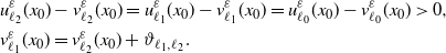 \begin{align*} &u^{\varepsilon}_{\ell_{2}}(x_{0})-v^{\varepsilon}_{\ell_{2}}(x_{0})=u^{\varepsilon}_{\ell_{1}}(x_{0})-v^{\varepsilon}_{\ell_{1}}(x_{0})=u^{\varepsilon}_{\ell_{0}}(x_{0})-v^{\varepsilon}_{\ell_{0}}(x_{0})>0,\notag\\ &v^{\varepsilon}_{\ell_{1}}(x_{0})=v^{\varepsilon}_{\ell_{2}}(x_{0})+\vartheta_{\ell_{1},\ell_{2}}. \end{align*}
Recursively, we obtain a sequence of regimes
 $\{\ell_{i}\}_{i\geq0}$
such that
$\{\ell_{i}\}_{i\geq0}$
such that
 \begin{align} &u^{\varepsilon}_{\ell_{i}}(x_{0})-v^{\varepsilon}_{\ell_{i}}(x_{0})=u^{\varepsilon}_{\ell_{i-1}}(x_{0})-v^{\varepsilon}_{\ell_{i-1}}(x_{0})=\cdots=u^{\varepsilon}_{\ell_{0}}(x_{0})-v^{\varepsilon}_{\ell_{0}}(x_{0})>0,\notag\\ &v^{\varepsilon}_{\ell_{i}}(x_{0})=v^{\varepsilon}_{\ell_{i+1}}(x_{0})+\vartheta_{\ell_{i},\ell_{i+1}}. \end{align}
Since
 $\mathbb{I}$
is finite, there is a regime
$\mathbb{I}$
is finite, there is a regime
 $\ell^{\prime}$
that will appear infinitely often in
$\ell^{\prime}$
that will appear infinitely often in
 $\{\ell_{i}\}_{i\geq0}$
. Let
$\{\ell_{i}\}_{i\geq0}$
. Let
 $\ell_{n}=\ell^{\prime}$
, for some
$\ell_{n}=\ell^{\prime}$
, for some
 $n>1$
. After
$n>1$
. After
 $\hat{n}$
steps, the regime
$\hat{n}$
steps, the regime
 $\ell^{\prime}$
reappears, i.e.
$\ell^{\prime}$
reappears, i.e.
 $\ell_{n+\hat{n}}=\ell^{\prime}$
. Then, by (3.23), we get
$\ell_{n+\hat{n}}=\ell^{\prime}$
. Then, by (3.23), we get
 \begin{equation} v^{\varepsilon}_{\ell^{\prime}}(x_{0})=v^{\varepsilon}_{\ell^{\prime}}(x_{0})+\vartheta_{\ell^{\prime},\ell_{n+1}}+\vartheta_{\ell_{n+1},\ell_{n+2}}+\cdots+\vartheta_{\ell_{n+\hat{n}-1},\ell^{\prime}}. \end{equation}
Notice that (3.24) contradicts the assumption that there is no loop of zero cost (see Equation (2.7)). From here we conclude that (3.15) must hold. Taking
 $v^{\varepsilon}-u^{\varepsilon}$
and proceeding in the same way as before, it follows that for each
$v^{\varepsilon}-u^{\varepsilon}$
and proceeding in the same way as before, it follows that for each
 $\ell\in\mathbb{I}$
,
$\ell\in\mathbb{I}$
,
 $v^{\varepsilon}_{\ell}-u^{\varepsilon}_{\ell}\leq 0$
in
$v^{\varepsilon}_{\ell}-u^{\varepsilon}_{\ell}\leq 0$
in
 $ \mathcal{O} $
, and hence we conclude that the solution
$ \mathcal{O} $
, and hence we conclude that the solution
 $u^{\varepsilon}$
to the HJB equation (2.20) is unique.
$u^{\varepsilon}$
to the HJB equation (2.20) is unique.
3.2. Proof of Theorem 2.1
In view of Lemma 3.1 and by (3.5), the following inequalities hold for each
 $\ell\in\mathbb{I}$
:
$\ell\in\mathbb{I}$
:
 \begin{equation}0\leq u^{\varepsilon}_{\ell}\leq C_{1}\quad\text{and}\quad \big|\textrm{D}^{1}u^{\varepsilon}_{\ell}\big|\leq C_{4},\quad\text{in}\ \overline{\mathcal{O}},\end{equation}
for some positive constant
 $C_{4}=C_{4}(d,\Lambda,\alpha^{\prime})$
. The constant
$C_{4}=C_{4}(d,\Lambda,\alpha^{\prime})$
. The constant
 $C_{1}$
is as in (3.2). Moreover, for each
$C_{1}$
is as in (3.2). Moreover, for each
 $B_{\beta r}\subset\mathcal{O}$
, there exists a positive constant
$B_{\beta r}\subset\mathcal{O}$
, there exists a positive constant
 $C_{5}=C_{5}(d,\Lambda,\alpha^{\prime})$
such that
$C_{5}=C_{5}(d,\Lambda,\alpha^{\prime})$
such that
 \begin{equation}\big|\big|\textrm{D}^{2}u^{\varepsilon}_{\ell}\big|\big|_{L^{p}\big(B_{\beta r}\big)}\leq C_{5},\quad \text{for each}\ p\in(1,\infty).\end{equation}
Then, from (3.25)–(3.26) and using again the Arzelà–Ascoli compactness criterion and the fact that
 $\Big(\text{L}^{p}\big(B_{\beta r}\big),||{\cdot}||_{L^{p}\big(B_{\beta r}\big)}\Big)$
is a reflexive space, we have that there exist a subsequence
$\Big(\text{L}^{p}\big(B_{\beta r}\big),||{\cdot}||_{L^{p}\big(B_{\beta r}\big)}\Big)$
is a reflexive space, we have that there exist a subsequence
 $\big\{u^{\varepsilon_{n}}_{\ell}\big\}_{n\geq1}$
of
$\big\{u^{\varepsilon_{n}}_{\ell}\big\}_{n\geq1}$
of
 $\big\{u^{\varepsilon}_{\ell}\big\}_{\varepsilon\in(0,1)}$
and a
$\big\{u^{\varepsilon}_{\ell}\big\}_{\varepsilon\in(0,1)}$
and a
 $u_{\ell}$
in
$u_{\ell}$
in
 $\textrm{C}^{0,1}\big(\overline{\mathcal{O}}\big)\cap \textrm{W}^{2,\infty}_{\textrm{loc}}(\mathcal{O})$
such that
$\textrm{C}^{0,1}\big(\overline{\mathcal{O}}\big)\cap \textrm{W}^{2,\infty}_{\textrm{loc}}(\mathcal{O})$
such that
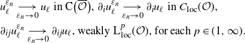 \begin{align}&\text{$u^{\varepsilon_{n}}_{\ell}\underset{\varepsilon_{n}\rightarrow0}{\longrightarrow}u_{\ell}$ in $\textrm{C}\big(\overline{\mathcal{O}}\big)$, $\partial_{i}u^{\varepsilon_{n}}_{\ell}\underset{\varepsilon_{n}\rightarrow0}{\longrightarrow}\partial_{i} u_{\ell}$ $\text{in}\ C_{\textrm{loc}}(\mathcal{O})$,}\\ &\text{$\partial_{ij}u^{\varepsilon_{n}}_{\ell}\underset{\varepsilon_{n}\rightarrow0}{\longrightarrow}\partial_{ij}u_{\ell}$, weakly $ \text{L}^{p}_{\textrm{loc}}(\mathcal{O})$, for each $p\in(1,\infty)$.}\end{align}
Remark 3.3. We use the notation
 $C=C(*,\dots,*)$
and
$C=C(*,\dots,*)$
and
 $K=K(*,\dots,*)$
to represent positive constants that depend only on the quantities appearing in parentheses.
$K=K(*,\dots,*)$
to represent positive constants that depend only on the quantities appearing in parentheses.
We proceed to proving Theorem 2.1.
Proof of Theorem 2.1. Existence. Now, let
 $\ell\in\mathbb{I}$
be fixed. Since
$\ell\in\mathbb{I}$
be fixed. Since
 $u^{\varepsilon_{n}}_{\ell}$
is the unique strong solution to the HJB equation (2.20) when
$u^{\varepsilon_{n}}_{\ell}$
is the unique strong solution to the HJB equation (2.20) when
 $\varepsilon=\varepsilon_{n}$
, which belongs to
$\varepsilon=\varepsilon_{n}$
, which belongs to
 $\text{C}^{0,1}\big(\overline{\mathcal{O}}\big)$
, it follows that for each
$\text{C}^{0,1}\big(\overline{\mathcal{O}}\big)$
, it follows that for each
 $\kappa\in\mathbb{I}\setminus\{\ell\}$
,
$\kappa\in\mathbb{I}\setminus\{\ell\}$
,
 $u^{\varepsilon_{n}}_{\ell}-\big(u^{\varepsilon_{n}}_{\kappa} +\vartheta_{\ell,\kappa}\big)\leq u^{\varepsilon_{n}}_{\ell}-\mathcal{M}_{\ell}u^{\varepsilon_{n}}\leq0$
in
$u^{\varepsilon_{n}}_{\ell}-\big(u^{\varepsilon_{n}}_{\kappa} +\vartheta_{\ell,\kappa}\big)\leq u^{\varepsilon_{n}}_{\ell}-\mathcal{M}_{\ell}u^{\varepsilon_{n}}\leq0$
in
 $\mathcal{O}$
. From here and (3.27), we have that
$\mathcal{O}$
. From here and (3.27), we have that
 $u_{\ell}-u_{\kappa} -\vartheta_{\ell,\kappa}\leq0$
in
$u_{\ell}-u_{\kappa} -\vartheta_{\ell,\kappa}\leq0$
in
 $\mathcal{O}$
. Then,
$\mathcal{O}$
. Then,
 $u_{\ell}-\mathcal{M}_{\ell}u\leq0$
, in
$u_{\ell}-\mathcal{M}_{\ell}u\leq0$
, in
 $\mathcal{O}$
. Also, we know that
$\mathcal{O}$
. Also, we know that
 $[c_{\ell}-\mathcal{L}_{\ell}] u_{\ell}^{\varepsilon_{n}}+ \psi_{\varepsilon_{n}}\Big(\big|\textrm{D}^{1} u_{\ell}^{\varepsilon_{n}}\big|^{2}- g_{\ell}^{2}\Big)\leq h_{\ell}$
a.e. in
$[c_{\ell}-\mathcal{L}_{\ell}] u_{\ell}^{\varepsilon_{n}}+ \psi_{\varepsilon_{n}}\Big(\big|\textrm{D}^{1} u_{\ell}^{\varepsilon_{n}}\big|^{2}- g_{\ell}^{2}\Big)\leq h_{\ell}$
a.e. in
 $\mathcal{O}$
. Thus,
$\mathcal{O}$
. Thus,
 \begin{align} &0\leq\psi_{\varepsilon_{n}}\Big(\big|\textrm{D}^{1} u_{\ell}^{\varepsilon_{n}}\big|^{2}- g_{\ell}^{2}\Big)\leq h_{\ell}-[c_{\ell}-\mathcal{L}_{\ell}] u_{\ell}^{\varepsilon_{n}},\quad \text{a.e.}\ \text{in}\ \mathcal{O}. \end{align}
Consequently, by (H3), (3.25), (3.26), and (3.28), there exists a positive constant
 $C_{6}=C_{6}(d,\Lambda,\alpha^{\prime})$
such that
$C_{6}=C_{6}(d,\Lambda,\alpha^{\prime})$
such that
 \begin{equation*}0\leq\int_{B_{r}}\psi_{\varepsilon_{n}}\Big(\big|\textrm{D}^{1} u_{\ell}^{\varepsilon_{n}}\big|^{2}- g_{\ell}^{2}\Big)\varpi\textrm{d} x\leq\int_{B_{r}} \big\{h_{\ell}-[c_{\ell}-\mathcal{L}_{\ell}] u_{\ell}^{\varepsilon_{n}}\big\}\varpi\textrm{d} x\leq C_{6}\end{equation*}
for each
 $\varpi\in\mathcal{B}(B_{r})$
, with
$\varpi\in\mathcal{B}(B_{r})$
, with
 $\mathcal{B}({\cdot})$
as in (3.8). Thus, using definition of
$\mathcal{B}({\cdot})$
as in (3.8). Thus, using definition of
 $\psi_{\varepsilon}$
(see (2.16)), and since
$\psi_{\varepsilon}$
(see (2.16)), and since
 $\big|\textrm{D}^{1}u_{\ell}^{\varepsilon_{n}}\big|^{2}-g^{2}_{\ell}$
is continuous in
$\big|\textrm{D}^{1}u_{\ell}^{\varepsilon_{n}}\big|^{2}-g^{2}_{\ell}$
is continuous in
 $\mathcal{O}$
, we have that for each
$\mathcal{O}$
, we have that for each
 $B_{r}\subset \mathcal{O}$
, there exists
$B_{r}\subset \mathcal{O}$
, there exists
 $\varepsilon^{\prime}\in(0,1)$
small enough so that for all
$\varepsilon^{\prime}\in(0,1)$
small enough so that for all
 $\varepsilon_{n}\leq \varepsilon^{\prime}$
,
$\varepsilon_{n}\leq \varepsilon^{\prime}$
,
 $\big|\textrm{D}^{1}u^{\varepsilon_{n}}_{\ell}\big|-g_{\ell}\leq0$
in
$\big|\textrm{D}^{1}u^{\varepsilon_{n}}_{\ell}\big|-g_{\ell}\leq0$
in
 $B_{r}$
. Then, since (3.27) holds, it follows that
$B_{r}$
. Then, since (3.27) holds, it follows that
 $|\textrm{D}^{1} u_{\ell}|\leq g_{\ell}$
in
$|\textrm{D}^{1} u_{\ell}|\leq g_{\ell}$
in
 $\mathcal{O}$
. From (3.28), we get
$\mathcal{O}$
. From (3.28), we get
 $\int_{B_{r}}\big\{[c_{\ell}-\mathcal{L}_{\ell}] u_{\ell}^{\varepsilon_{n}}-h_{\ell}\big\}\varpi\textrm{d} x\leq 0$
, for each
$\int_{B_{r}}\big\{[c_{\ell}-\mathcal{L}_{\ell}] u_{\ell}^{\varepsilon_{n}}-h_{\ell}\big\}\varpi\textrm{d} x\leq 0$
, for each
 $\varpi\in \mathcal{B}(B_{r})$
. From here and (3.27), we obtain that
$\varpi\in \mathcal{B}(B_{r})$
. From here and (3.27), we obtain that
 $[c_{\ell}-\mathcal{L}_{\ell}] u_{\ell}-h_{\ell}\leq 0$
a.e. in
$[c_{\ell}-\mathcal{L}_{\ell}] u_{\ell}-h_{\ell}\leq 0$
a.e. in
 $\mathcal{O}$
. Therefore, by what we saw previously,
$\mathcal{O}$
. Therefore, by what we saw previously,
 \begin{equation} \max\Big\{[c_{\ell}-\mathcal{L}_{\ell}] u_{\ell}-h_{\ell},\big|\textrm{D}^{1} u_{\ell}\big|- g_{\ell},u_{\ell}-\mathcal{M}_{\ell}u\Big\}\leq 0 ,\quad \text{a.e.}\ \text{in}\ \mathcal{O}. \end{equation}
Without loss of generality we assume that
 $ u_{\ell}(x^{*})-\mathcal{M}_{\ell}u(x^{*})<0$
, for some
$ u_{\ell}(x^{*})-\mathcal{M}_{\ell}u(x^{*})<0$
, for some
 $x^{*}\in\mathcal{O}$
. Otherwise, equality holds in (3.29). Then, for each
$x^{*}\in\mathcal{O}$
. Otherwise, equality holds in (3.29). Then, for each
 $\kappa\in\mathbb{I}$
such that
$\kappa\in\mathbb{I}$
such that
 $\kappa\neq\ell$
,
$\kappa\neq\ell$
,
 $u_{\ell}-(u_{\kappa} +\vartheta_{\ell,\kappa})\leq u_{\ell}-\mathcal{M}_{\ell}u<0$
at
$u_{\ell}-(u_{\kappa} +\vartheta_{\ell,\kappa})\leq u_{\ell}-\mathcal{M}_{\ell}u<0$
at
 $x^{*}$
. There exists a ball
$x^{*}$
. There exists a ball
 $B_{r_{1}}(x^{*})\subset\mathcal{O}$
such that
$B_{r_{1}}(x^{*})\subset\mathcal{O}$
such that
 \begin{equation} u_{\ell}-(u_{\kappa} +\vartheta_{\ell,\kappa})\leq u_{\ell}-\mathcal{M}_{\ell}u<0,\quad\text{in}\ B_{r_{1}}(x^{*}), \end{equation}
by the continuity of
 $u_{\ell}-u_{\kappa}$
in
$u_{\ell}-u_{\kappa}$
in
 $\overline{\mathcal{O}}$
. Now, consider that
$\overline{\mathcal{O}}$
. Now, consider that
 $\big|\textrm{D}^{1}u_{\ell}\big|-g_{\ell}<0$
for some
$\big|\textrm{D}^{1}u_{\ell}\big|-g_{\ell}<0$
for some
 $x^{*}_{1}\in B_{r_{1}}(x^{*})$
. Otherwise, equality again holds in (3.29). By continuity of
$x^{*}_{1}\in B_{r_{1}}(x^{*})$
. Otherwise, equality again holds in (3.29). By continuity of
 $\big|\textrm{D}^{1}u_{\ell}\big|-g_{\ell}$
, we have that for some
$\big|\textrm{D}^{1}u_{\ell}\big|-g_{\ell}$
, we have that for some
 $B_{r_{2}}(x^{*}_{1})\subset\mathcal{O}$
,
$B_{r_{2}}(x^{*}_{1})\subset\mathcal{O}$
,
 $\big|\textrm{D}^{1}u_{\ell}\big|-g_{\ell}<0$
in
$\big|\textrm{D}^{1}u_{\ell}\big|-g_{\ell}<0$
in
 $B_{r_{2}}(x^{*}_{1})$
. From here, using (3.27), (3.30) and taking
$B_{r_{2}}(x^{*}_{1})$
. From here, using (3.27), (3.30) and taking
 $\mathcal{N}\,:\!=\, B_{r_{1}}(x^{*})\cap B_{r_{2}}\big(x^{*}_{1}\big)$
, it can be verified that there exists an
$\mathcal{N}\,:\!=\, B_{r_{1}}(x^{*})\cap B_{r_{2}}\big(x^{*}_{1}\big)$
, it can be verified that there exists an
 $\varepsilon^{\prime}\in(0,1)$
small enough so that for each
$\varepsilon^{\prime}\in(0,1)$
small enough so that for each
 $\varepsilon_{n}\leq\varepsilon^{\prime}$
,
$\varepsilon_{n}\leq\varepsilon^{\prime}$
,
 $|\textrm{D}^{1}u^{\varepsilon_{n}}_{\ell}|-g_{\ell}<0$
and
$|\textrm{D}^{1}u^{\varepsilon_{n}}_{\ell}|-g_{\ell}<0$
and
 $ u^{\varepsilon_{n}}_{\ell}-\mathcal{M}_{\ell}u^{\varepsilon_{n}}<0$
in
$ u^{\varepsilon_{n}}_{\ell}-\mathcal{M}_{\ell}u^{\varepsilon_{n}}<0$
in
 $\mathcal{N}$
. Thus,
$\mathcal{N}$
. Thus,
 $[c_{\ell}-\mathcal{L}_{\ell}] u_{\ell}^{\varepsilon_{n}}= h_{\ell}$
a.e. in
$[c_{\ell}-\mathcal{L}_{\ell}] u_{\ell}^{\varepsilon_{n}}= h_{\ell}$
a.e. in
 $\mathcal{N}$
, since
$\mathcal{N}$
, since
 $u^{\varepsilon_{n}}$
is the unique solution to the HJB equation (2.20), when
$u^{\varepsilon_{n}}$
is the unique solution to the HJB equation (2.20), when
 $\varepsilon=\varepsilon_{n}$
. Then,
$\varepsilon=\varepsilon_{n}$
. Then,
 $\int_{\mathcal{N}}\big\{[c_{\ell}-\mathcal{L}_{\ell}] u_{\ell}^{\varepsilon_{n}}-h_{\ell}\big\}\varpi\textrm{d} x= 0$
, for each
$\int_{\mathcal{N}}\big\{[c_{\ell}-\mathcal{L}_{\ell}] u_{\ell}^{\varepsilon_{n}}-h_{\ell}\big\}\varpi\textrm{d} x= 0$
, for each
 $\varpi\in\mathcal{B}(\mathcal{N})$
. Hence, letting
$\varpi\in\mathcal{B}(\mathcal{N})$
. Hence, letting
 $\varepsilon_{n}\rightarrow0$
and again using (3.27), we get that
$\varepsilon_{n}\rightarrow0$
and again using (3.27), we get that
 $u=(u_{1},\dots,u_{m})$
is a solution to the HJB equation (2.9).
$u=(u_{1},\dots,u_{m})$
is a solution to the HJB equation (2.9).
Proof of Theorem 2.1. Uniqueness. Suppose that
 \begin{equation*}u=(u_{1},\dots,u_{m})\quad \text{and}\quad v=(v_{1},\dots,v_{m})\end{equation*}
are two solutions to the HJB equation (2.9) whose components belong to
 $\textrm{C}^{0,1}\big(\overline{\mathcal{O}}\big)\cap \textrm{W}^{2,\infty}_{\textrm{loc}}(\mathcal{O})$
. Take
$\textrm{C}^{0,1}\big(\overline{\mathcal{O}}\big)\cap \textrm{W}^{2,\infty}_{\textrm{loc}}(\mathcal{O})$
. Take
 $(x_{0},\ell_{0})\in\overline{\mathcal{O}}\times\mathbb{I}$
such that
$(x_{0},\ell_{0})\in\overline{\mathcal{O}}\times\mathbb{I}$
such that
 \begin{equation} u_{\ell_{0}}(x_{0})-v_{\ell_{0}}(x_{0})=\sup_{(x,\ell)\in\overline{\mathcal{O}}\times\mathbb{I}}\{u_{\ell}(x)-v_{\ell}(x)\}. \end{equation}
As before (see Subsection 3.1), we only need to verify that
 \begin{equation} u_{\ell_{0}}-v_{\ell_{0}}\leq0,\quad \text{at}\ x_{0}\in\mathcal{O}. \end{equation}
Assume that
 $u_{\ell_{0}}-v_{\ell_{0}}>0$
at
$u_{\ell_{0}}-v_{\ell_{0}}>0$
at
 $x_{0}$
. Then there exists a ball
$x_{0}$
. Then there exists a ball
 $B_{r_{1}}(x_{0})\subset\mathcal{O}$
such that
$B_{r_{1}}(x_{0})\subset\mathcal{O}$
such that
 \begin{equation*}c_{\ell_{0}}[u_{\ell_{0}}-v_{\ell_{0}}]\geq\min_{x\in B_{r_{1}}(x_{0})}\big\{c_{\ell_{0}}(x)\big[u_{\ell_{0}}(x)-v_{\ell_{0}}(x)\big]\big\}>0\end{equation*}
in
 $B_{r_{1}}(x_{0}),$
by the continuity of
$B_{r_{1}}(x_{0}),$
by the continuity of
 $u_{\ell_{0}}-v_{\ell_{0}}$
in
$u_{\ell_{0}}-v_{\ell_{0}}$
in
 $\overline{\mathcal{O}}$
and the fact that
$\overline{\mathcal{O}}$
and the fact that
 $c_{\ell_{0}}>0$
in
$c_{\ell_{0}}>0$
in
 $\mathcal{O}$
. Meanwhile, from (3.31),
$\mathcal{O}$
. Meanwhile, from (3.31),
 $v_{\ell_{0}}-\mathcal{M}_{\ell_{0}}v\leq u_{\ell_{0}}-\mathcal{M}_{\ell_{0}}u\leq 0$
at
$v_{\ell_{0}}-\mathcal{M}_{\ell_{0}}v\leq u_{\ell_{0}}-\mathcal{M}_{\ell_{0}}u\leq 0$
at
 $x_{0}$
. If
$x_{0}$
. If
 $v_{\ell_{0}}-\mathcal{M}_{\ell_{0}}v<0$
at
$v_{\ell_{0}}-\mathcal{M}_{\ell_{0}}v<0$
at
 $x_{0}$
, there exists a ball
$x_{0}$
, there exists a ball
 $B_{r_{2}}(x_{0})\subset\mathcal{O}$
such that
$B_{r_{2}}(x_{0})\subset\mathcal{O}$
such that
 $v_{\ell_{0}}-\mathcal{M}_{\ell_{0}}v<0$
in
$v_{\ell_{0}}-\mathcal{M}_{\ell_{0}}v<0$
in
 $B_{r_{2}}(x_{0})$
. Now, consider the auxiliary function
$B_{r_{2}}(x_{0})$
. Now, consider the auxiliary function
 $f_{\varrho}\,:\!=\, u_{\ell_{0}}-v_{\ell_{0}}-\varrho u_{\ell_{0}}$
, with
$f_{\varrho}\,:\!=\, u_{\ell_{0}}-v_{\ell_{0}}-\varrho u_{\ell_{0}}$
, with
 $\varrho\in(0,1)$
. Notice that
$\varrho\in(0,1)$
. Notice that
 $f_{\varrho}=0$
on
$f_{\varrho}=0$
on
 $\partial\mathcal{O}$
, for
$\partial\mathcal{O}$
, for
 $\varrho\in(0,1)$
, and
$\varrho\in(0,1)$
, and
 \begin{equation} f_{\varrho}\uparrow u_{\ell_{0}}-v_{\ell_{0}}\ \text{uniformly in}\ \mathcal{O},\ \text{when}\ \varrho\downarrow 0. \end{equation}
In addition, there is a
 $\varrho^{\prime}\in(0,1)$
small enough so that
$\varrho^{\prime}\in(0,1)$
small enough so that
 $\sup_{x\in B_{r_{2}}(x_{0})}\{f_{\varrho}(x)\}>0$
for all
$\sup_{x\in B_{r_{2}}(x_{0})}\{f_{\varrho}(x)\}>0$
for all
 $\varrho\in(0,\varrho^{\prime})$
, since
$\varrho\in(0,\varrho^{\prime})$
, since
 $u_{\ell_{0}}-v_{\ell_{0}}>0$
at
$u_{\ell_{0}}-v_{\ell_{0}}>0$
at
 $x_{0}$
. By (3.31) and (3.33), there exists
$x_{0}$
. By (3.31) and (3.33), there exists
 $\hat{\varrho}\in(0,\varrho^{\prime})$
small enough so that
$\hat{\varrho}\in(0,\varrho^{\prime})$
small enough so that
 $f_{\hat{\varrho}}$
has a local maximum at
$f_{\hat{\varrho}}$
has a local maximum at
 $x_{\hat{\varrho}}\in B_{r_{1}}(x_{0})\cap B_{r_{2}}(x_{0})$
. It follows that
$x_{\hat{\varrho}}\in B_{r_{1}}(x_{0})\cap B_{r_{2}}(x_{0})$
. It follows that
 \begin{equation*}\big|\textrm{D}^{1}v_{\ell_{0}}\big(x_{\hat{\varrho}}\big)\big|=[1-\hat{\varrho}]\big|\textrm{D}^{1}u_{\ell_{0}}\big(x_{\hat{\varrho}}\big)\big|<\big|\textrm{D}^{1}u_{\ell_{0}}\big(x_{\hat{\varrho}}\big)\big|\leq g\big(x_{\hat{\varrho}}\big).\end{equation*}
Thus, there exists a ball
 $B_{r_{3}}\big(x_{\hat{\varrho}}\big)\subset B_{r_{1}}(x_{0})\cap B_{r_{2}}(x_{0})$
such that
$B_{r_{3}}\big(x_{\hat{\varrho}}\big)\subset B_{r_{1}}(x_{0})\cap B_{r_{2}}(x_{0})$
such that
 $[c_{\ell_{0}}-\mathcal{L}_{\ell_{0}}] v_{\ell_{0}}-h_{\ell_{0}}=0$
and
$[c_{\ell_{0}}-\mathcal{L}_{\ell_{0}}] v_{\ell_{0}}-h_{\ell_{0}}=0$
and
 $[c_{\ell_{0}}-\mathcal{L}_{\ell_{0}}] u_{\ell_{0}}-h_{\ell_{0}}\leq0$
in
$[c_{\ell_{0}}-\mathcal{L}_{\ell_{0}}] u_{\ell_{0}}-h_{\ell_{0}}\leq0$
in
 $B_{r_{3}}\big(x_{\hat{{\varrho}}}\big)$
. Then, by Bony’s maximum principle, we have that
$B_{r_{3}}\big(x_{\hat{{\varrho}}}\big)$
. Then, by Bony’s maximum principle, we have that
 $$\begin{equation*}0\geq\lim_{r\rightarrow0}\bigg\{\mathop{\textrm{inf} \, \textrm{ess}}\limits_{B_{r}\big(x_{\hat{\varrho}}\big)} \textrm{tr}\Big[a_{\ell_{0}}\textrm{D}^{2}f_{\hat{\varrho}}\Big]\bigg\}\geq c_{\ell_{0}}f_{\hat{\varrho}}+\hat{\varrho} h_{\ell_{0}}\end{equation*}$$
at
 $x_{\hat{\varrho}},$
which is a contradiction since
$x_{\hat{\varrho}},$
which is a contradiction since
 $\hat{\varrho} h_{\ell}\geq0$
,
$\hat{\varrho} h_{\ell}\geq0$
,
 $f_{\hat{\varrho}}>0$
, and
$f_{\hat{\varrho}}>0$
, and
 $c_{\ell_{0}}>0$
at
$c_{\ell_{0}}>0$
at
 $x_{\hat{\varrho}}$
. We conclude that
$x_{\hat{\varrho}}$
. We conclude that
 $0=v_{\ell_{0}}-\mathcal{M}_{\ell_{0}}v\leq u_{\ell_{0}}-\mathcal{M}_{\ell_{0}}u\leq 0$
at
$0=v_{\ell_{0}}-\mathcal{M}_{\ell_{0}}v\leq u_{\ell_{0}}-\mathcal{M}_{\ell_{0}}u\leq 0$
at
 $x_{0}$
. Using the same arguments seen in the proof of uniqueness of the solution to the HJB equation (2.9) (see Subsection 3.1), it can be verified that there is a contradiction with the assumption that there is no loop of zero cost (see Equation (2.7)). From here we conclude that ((3.32)) must hold. Taking
$x_{0}$
. Using the same arguments seen in the proof of uniqueness of the solution to the HJB equation (2.9) (see Subsection 3.1), it can be verified that there is a contradiction with the assumption that there is no loop of zero cost (see Equation (2.7)). From here we conclude that ((3.32)) must hold. Taking
 $v-u$
and proceeding in the same way as before, we see that u is the unique solution to the HJB equation (2.9).
$v-u$
and proceeding in the same way as before, we see that u is the unique solution to the HJB equation (2.9).
4. Verification lemma for
$\varepsilon$
-PACS control problem and proof of Theorem 2.2

In this section, under Assumptions (H1) and (H3)–(H5), we shall verify that the value function V given in (2.8) agrees with the solution u to the HJB equation (2.9) on
 $\overline{\mathcal{O}}$
. To that end, let us start by showing that the value function
$\overline{\mathcal{O}}$
. To that end, let us start by showing that the value function
 $V^{\varepsilon}$
given in (2.18), with
$V^{\varepsilon}$
given in (2.18), with
 $\varepsilon\in(0,1)$
fixed, agrees with the solution
$\varepsilon\in(0,1)$
fixed, agrees with the solution
 $u^{\varepsilon}$
to (2.20). The proof of this result is presented in two parts; see Lemmas 4.1 and 4.2.
$u^{\varepsilon}$
to (2.20). The proof of this result is presented in two parts; see Lemmas 4.1 and 4.2.
Let us assume that
 $ \big(X^{\xi,\varsigma},I^{\varsigma}\big)$
evolves as (2.14)–(2.15), with
$ \big(X^{\xi,\varsigma},I^{\varsigma}\big)$
evolves as (2.14)–(2.15), with
 $(\xi,\varsigma)\in\mathcal{U}^{\varepsilon}\times\mathcal{S}$
and initial state
$(\xi,\varsigma)\in\mathcal{U}^{\varepsilon}\times\mathcal{S}$
and initial state
 $\big(\tilde{x},\tilde{\ell}\big)\in {\mathcal{O}}\times\mathbb{I}$
. Recall that
$\big(\tilde{x},\tilde{\ell}\big)\in {\mathcal{O}}\times\mathbb{I}$
. Recall that
 $\mathcal{U}^{\varepsilon}$
is defined in (2.13) and
$\mathcal{U}^{\varepsilon}$
is defined in (2.13) and
 $\mathcal{S}$
is the set of elements
$\mathcal{S}$
is the set of elements
 $\varsigma=(\tau_{i},\ell_{i})_{i\geq0}$
that satisfy (2.2). The functional cost
$\varsigma=(\tau_{i},\ell_{i})_{i\geq0}$
that satisfy (2.2). The functional cost
 $\mathcal{V}_{\xi,\varsigma}$
is as in (2.17).
$\mathcal{V}_{\xi,\varsigma}$
is as in (2.17).
Under Assumptions (H1)–(H4), Lemmas 4.1 and 4.3 will be proven.
Lemma 4.1. (Verification lemma for
 $\varepsilon$
-PACS control problem, first part) Let
$\varepsilon$
-PACS control problem, first part) Let
 $\varepsilon\in(0,1)$
be fixed. Then
$\varepsilon\in(0,1)$
be fixed. Then
 $u^{\varepsilon}_{\tilde{\ell}}(\tilde{x})\leq\mathcal{V}_{\zeta,\varsigma}\big(\tilde{x},\tilde{\ell}\big)$
for each
$u^{\varepsilon}_{\tilde{\ell}}(\tilde{x})\leq\mathcal{V}_{\zeta,\varsigma}\big(\tilde{x},\tilde{\ell}\big)$
for each
 $\big(\tilde{x},\tilde{\ell}\big)\in\overline{\mathcal{O}}\times\mathbb{I}$
and
$\big(\tilde{x},\tilde{\ell}\big)\in\overline{\mathcal{O}}\times\mathbb{I}$
and
 $(\xi,\varsigma)\in\mathcal{U}^{\varepsilon}\times\mathcal{S}$
. From now on, for simplicity of notation, we replace
$(\xi,\varsigma)\in\mathcal{U}^{\varepsilon}\times\mathcal{S}$
. From now on, for simplicity of notation, we replace
 $X^{\xi,\varsigma}$
by X in the proofs of the results.
$X^{\xi,\varsigma}$
by X in the proofs of the results.
Proof of Lemma 4.1. Let
 $\{u^{\varepsilon,\delta_{\hat{n}}}\}_{\hat{n}\geq1}$
be the sequence of unique solutions to the NPDS (3.1), when
$\{u^{\varepsilon,\delta_{\hat{n}}}\}_{\hat{n}\geq1}$
be the sequence of unique solutions to the NPDS (3.1), when
 $\delta=\delta_{\hat{n}}$
, which satisfy (3.5). By Proposition 3.1, it is known that
$\delta=\delta_{\hat{n}}$
, which satisfy (3.5). By Proposition 3.1, it is known that
 $u^{\varepsilon,\delta_{\hat{n}}}_{\ell}\in \textrm{C}^{4,\alpha^{\prime}}\big(\overline{\mathcal{O}}\big)$
for
$u^{\varepsilon,\delta_{\hat{n}}}_{\ell}\in \textrm{C}^{4,\alpha^{\prime}}\big(\overline{\mathcal{O}}\big)$
for
 $\ell\in\mathbb{I}$
. Then, using integration by parts and Itô’s formula (see Corollary 2 (p. 68) and Theorem 33 (p. 81), respectively, in [Reference Protter17]) in
$\ell\in\mathbb{I}$
. Then, using integration by parts and Itô’s formula (see Corollary 2 (p. 68) and Theorem 33 (p. 81), respectively, in [Reference Protter17]) in ![]() on
on
 $ \big[\tilde{\tau}_{i},\tilde{\tau}_{i+1}\big)$
,
$ \big[\tilde{\tau}_{i},\tilde{\tau}_{i+1}\big)$
,
 $i\geq0$
, where
$i\geq0$
, where
 $\tilde{\tau}_{i}=\tau_{i}\wedge\tau$
,
$\tilde{\tau}_{i}=\tau_{i}\wedge\tau$
, ![]() and
and ![]() is as in (2.4), and taking the expected value, we have that
is as in (2.4), and taking the expected value, we have that

where
Since ![]() is a square-integrable martingale,
is a square-integrable martingale,
 \begin{equation*}\langle\gamma,y\rangle\leq\psi_{\varepsilon}\big(|\gamma|^{2}-g_{\ell} (x)^{2}\big)+l^{\varepsilon}_{\ell}(y,x),\end{equation*}
and
 \begin{equation*}[c_{\ell}-\mathcal{L}_{\ell}]u^{\varepsilon,\delta_{\hat{n}}}_{\ell}+\psi_{\varepsilon}\Big(\big|\textrm{D}^{1}u^{\varepsilon,\delta_{\hat{n}}}_{\ell}\big|^{2}-g^{2}_{\ell}\Big)\leq h_{\ell},\end{equation*}
it follows that

where
We have
by Lemma 3.1. Meanwhile, we know that
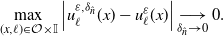 \begin{equation*}\max_{(x,\ell)\in\mathcal{O}\times\mathbb{I}}\Big|u^{\varepsilon,\delta_{\hat{n}}}_{\ell}(x)-u^{\varepsilon}_{\ell}(x)\Big|\underset{\delta_{\hat{n}}\rightarrow0}{\longrightarrow}0.\end{equation*}
Then, letting first
 $\delta_{\hat{n}}{\rightarrow}0$
and then
$\delta_{\hat{n}}{\rightarrow}0$
and then ![]() in (4.3), and by the dominated convergence theorem, we obtain that
in (4.3), and by the dominated convergence theorem, we obtain that
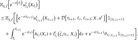
for
 $i\geq0$
. Observe that
$i\geq0$
. Observe that
 $\mathcal{D}\big[\tau_{i+1},\ell_{i},\ell_{i+1},X, u^{\varepsilon}\big]\unicode{x1D7D9}_{\{\tau_{i+1}<\tau\}}\leq0$
for
$\mathcal{D}\big[\tau_{i+1},\ell_{i},\ell_{i+1},X, u^{\varepsilon}\big]\unicode{x1D7D9}_{\{\tau_{i+1}<\tau\}}\leq0$
for
 $i\geq0$
since
$i\geq0$
since
 $u^{\varepsilon}_{\ell}-\big(u^{\varepsilon}_{\kappa} +\vartheta_{\ell,\kappa}\big)\leq u^{\varepsilon}_{\ell}-\mathcal{M}_{\ell}u^{\varepsilon}\leq0$
. From this remark and (4.5), we deduce the statement of the lemma above.
$u^{\varepsilon}_{\ell}-\big(u^{\varepsilon}_{\kappa} +\vartheta_{\ell,\kappa}\big)\leq u^{\varepsilon}_{\ell}-\mathcal{M}_{\ell}u^{\varepsilon}\leq0$
. From this remark and (4.5), we deduce the statement of the lemma above.
4.1.
$\varepsilon$
-PACS optimal control problem

Before presenting the second part of the verification lemma and proving it, we first construct the control
 $\big(\xi^{\varepsilon,*},\varsigma^{\varepsilon,*}\big)$
which turns out to be the optimal strategy for the
$\big(\xi^{\varepsilon,*},\varsigma^{\varepsilon,*}\big)$
which turns out to be the optimal strategy for the
 $\varepsilon$
-PACS control problem. To that end, let us introduce the switching regions.
$\varepsilon$
-PACS control problem. To that end, let us introduce the switching regions.
For any
 $\ell\in\mathbb{I}$
, let
$\ell\in\mathbb{I}$
, let
 $\mathcal{S}^{\varepsilon}_{\ell}$
be the set defined by
$\mathcal{S}^{\varepsilon}_{\ell}$
be the set defined by
 \begin{equation*}\mathcal{S}^{\varepsilon}_{\ell}=\Big\{x\in\mathcal{O}\,:\,u^{\varepsilon}_{\ell}(x)-\mathcal{M}_{\ell}u^{\varepsilon}(x)=0\Big\}.\end{equation*}
Notice that
 $\mathcal{S}^{\varepsilon}_{\ell}$
is a closed subset of
$\mathcal{S}^{\varepsilon}_{\ell}$
is a closed subset of
 $\mathcal{O}$
and corresponds to the region where it is optimal to switch regimes. The complement
$\mathcal{O}$
and corresponds to the region where it is optimal to switch regimes. The complement
 $\mathcal{C}^{\varepsilon}_{\ell}$
of
$\mathcal{C}^{\varepsilon}_{\ell}$
of
 $\mathcal{S}^{\varepsilon}_{\ell}$
in
$\mathcal{S}^{\varepsilon}_{\ell}$
in
 $\mathcal{O}$
, where it is optimal to stay in the regime
$\mathcal{O}$
, where it is optimal to stay in the regime
 $\ell$
, is the so-called continuation region
$\ell$
, is the so-called continuation region
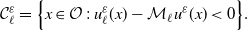 \begin{equation*}\mathcal{C}^{\varepsilon}_{\ell}=\Big\{x\in\mathcal{O}\,:\,u^{\varepsilon}_{\ell}(x)-\mathcal{M}_{\ell}u^{\varepsilon}(x)<0\Big\}.\end{equation*}
Remark 4.1. Observe that
 $u^{\varepsilon}_{\ell}\in W^{2,\infty}_{\textrm{loc}}\big(\mathcal{C}^{\varepsilon}_{\ell}\big)=C_{\textrm{loc}}^{1,1}\big(\mathcal{C}^{\varepsilon}_{\ell}\big)$
. This implies that
$u^{\varepsilon}_{\ell}\in W^{2,\infty}_{\textrm{loc}}\big(\mathcal{C}^{\varepsilon}_{\ell}\big)=C_{\textrm{loc}}^{1,1}\big(\mathcal{C}^{\varepsilon}_{\ell}\big)$
. This implies that
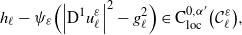 \begin{equation*}h_{\ell}-\psi_{\varepsilon}\Big(\Big|\textrm{D}^{1}u^{\varepsilon}_{\ell}\Big|^{2}-g_{\ell}^{2}\Big)\in \textrm{C}^{0,\alpha^{\prime}}_{\textrm{loc}}\big(\mathcal{C}_{\ell}^{\varepsilon}\big),\end{equation*}
since
 $h_{\ell}\in \textrm{C}^{2,\alpha^{\prime}}\big(\overline{\mathcal{O}}\big))$
and
$h_{\ell}\in \textrm{C}^{2,\alpha^{\prime}}\big(\overline{\mathcal{O}}\big))$
and
 $\psi_{\varepsilon}\Big(\big|\textrm{D}^{1}u^{\varepsilon}_{\ell}\big|^{2}-g_{\ell}^{2}\Big)\in \text{C}^{0,\alpha^{\prime}}_{\textrm{loc}}\big(\mathcal{C}_{\ell}^{\varepsilon}\big)$
. From here and using Theorem 9.19 of [Reference Gilbarg and Trudinger10], we have that
$\psi_{\varepsilon}\Big(\big|\textrm{D}^{1}u^{\varepsilon}_{\ell}\big|^{2}-g_{\ell}^{2}\Big)\in \text{C}^{0,\alpha^{\prime}}_{\textrm{loc}}\big(\mathcal{C}_{\ell}^{\varepsilon}\big)$
. From here and using Theorem 9.19 of [Reference Gilbarg and Trudinger10], we have that
 $u^{\varepsilon}_{\ell}\in \text{C}_{\textrm{loc}}^{2,\alpha^{\prime}}\big(\mathcal{C}^{\varepsilon}_{\ell}\big)$
.
$u^{\varepsilon}_{\ell}\in \text{C}_{\textrm{loc}}^{2,\alpha^{\prime}}\big(\mathcal{C}^{\varepsilon}_{\ell}\big)$
.
Remark 4.2. Notice that there are no isolated points in a switching region
 $\mathcal{S}_{\ell}^{\varepsilon}$
.
$\mathcal{S}_{\ell}^{\varepsilon}$
.
Also, the set
 $\mathcal{S}^{\varepsilon}_{\ell}$
satisfies the following property.
$\mathcal{S}^{\varepsilon}_{\ell}$
satisfies the following property.
Lemma 4.2. Let
 $\ell$
be in
$\ell$
be in
 $\mathbb{I}$
. Then
$\mathbb{I}$
. Then
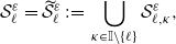 \begin{equation*}\mathcal{S}^{\varepsilon}_{\ell}=\widetilde{\mathcal{S}}^{\varepsilon}_{\ell}\,:\!=\,\bigcup_{\kappa\in\mathbb{I}\setminus\{\ell \}}\mathcal{S}^{\varepsilon}_{\ell,\kappa},\end{equation*}
where
 $\mathcal{S}^{\varepsilon}_{\ell,\kappa}\,:\!=\,\big\{x\in\mathcal{C}^{\varepsilon}_{\kappa}\,:\,u^{\varepsilon}_{\ell}(x)=u^{\varepsilon}_{\kappa}(x )+\vartheta_{\ell,\kappa} \big\}$
.
$\mathcal{S}^{\varepsilon}_{\ell,\kappa}\,:\!=\,\big\{x\in\mathcal{C}^{\varepsilon}_{\kappa}\,:\,u^{\varepsilon}_{\ell}(x)=u^{\varepsilon}_{\kappa}(x )+\vartheta_{\ell,\kappa} \big\}$
.
Proof. We obtain trivially that
 $\widetilde{\mathcal{S}}^{\varepsilon}_{\ell}\subset\mathcal{S}^{\varepsilon}_{\ell}$
, since
$\widetilde{\mathcal{S}}^{\varepsilon}_{\ell}\subset\mathcal{S}^{\varepsilon}_{\ell}$
, since
 $u^{\varepsilon}_{\ell}-u^{\varepsilon}_{\kappa}-\vartheta_{\ell,\kappa}\leq u^{\varepsilon}_{\ell}-\mathcal{M}_{\ell}u^{\varepsilon}\leq0$
on
$u^{\varepsilon}_{\ell}-u^{\varepsilon}_{\kappa}-\vartheta_{\ell,\kappa}\leq u^{\varepsilon}_{\ell}-\mathcal{M}_{\ell}u^{\varepsilon}\leq0$
on
 $\mathcal{O}$
for
$\mathcal{O}$
for
 $\kappa\in\mathbb{I}\setminus\{\ell\}$
. If
$\kappa\in\mathbb{I}\setminus\{\ell\}$
. If
 $x\in\mathcal{S}^{\varepsilon}_{\ell}$
, there is an
$x\in\mathcal{S}^{\varepsilon}_{\ell}$
, there is an
 $\ell_{1}\neq\ell$
where
$\ell_{1}\neq\ell$
where
 $u^{\varepsilon}_{\ell}(x)=u^{\varepsilon}_{\ell_{1}}(x)+\vartheta_{\ell,\ell_{1}}$
. Notice that x must belong to either
$u^{\varepsilon}_{\ell}(x)=u^{\varepsilon}_{\ell_{1}}(x)+\vartheta_{\ell,\ell_{1}}$
. Notice that x must belong to either
 $\mathcal{C}^{\varepsilon}_{\ell_{1}}$
or
$\mathcal{C}^{\varepsilon}_{\ell_{1}}$
or
 $\mathcal{S}^{\varepsilon}_{\ell_{1}}$
. If
$\mathcal{S}^{\varepsilon}_{\ell_{1}}$
. If
 $x\in\mathcal{C}^{\varepsilon}_{\ell_{1}}$
, then
$x\in\mathcal{C}^{\varepsilon}_{\ell_{1}}$
, then
 $x\in\mathcal{S}^{\varepsilon}_{\ell,\ell_{1}}\subset\widetilde{\mathcal{S}}^{\varepsilon}_{\ell} $
. Otherwise, there is an
$x\in\mathcal{S}^{\varepsilon}_{\ell,\ell_{1}}\subset\widetilde{\mathcal{S}}^{\varepsilon}_{\ell} $
. Otherwise, there is an
 $\ell_{2}\neq\ell_{1}$
such that
$\ell_{2}\neq\ell_{1}$
such that
 $u^{\varepsilon}_{\ell_{1}}\!(x)=u^{\varepsilon}_{\ell_{2}}(x)+\vartheta_{\ell_{1},\ell_{2}}$
. This implies
$u^{\varepsilon}_{\ell_{1}}\!(x)=u^{\varepsilon}_{\ell_{2}}(x)+\vartheta_{\ell_{1},\ell_{2}}$
. This implies
 \begin{equation*}u^{\varepsilon}_{\ell}(x)=u^{\varepsilon}_{\ell_{2}}(x)+\vartheta_{\ell,\ell_{1}}+\vartheta_{\ell_{1},\ell_{2}}\geq u^{\varepsilon}_{\ell_{2}}(x)+\vartheta_{\ell,\ell_{2}},\end{equation*}
since (2.6) holds. Then,
 $u^{\varepsilon}_{\ell}(x)= u^{\varepsilon}_{\ell_{2}}(x)+\vartheta_{\ell,\ell_{2}}$
. Again x must belong to either
$u^{\varepsilon}_{\ell}(x)= u^{\varepsilon}_{\ell_{2}}(x)+\vartheta_{\ell,\ell_{2}}$
. Again x must belong to either
 $\mathcal{C}^{\varepsilon}_{\ell_{2}}$
or
$\mathcal{C}^{\varepsilon}_{\ell_{2}}$
or
 $\mathcal{S}^{\varepsilon}_{\ell_{2}}$
. If
$\mathcal{S}^{\varepsilon}_{\ell_{2}}$
. If
 $x\in\mathcal{C}^{\varepsilon}_{\ell_{2}}$
, we have
$x\in\mathcal{C}^{\varepsilon}_{\ell_{2}}$
, we have
 $x\in\mathcal{S}^{\varepsilon}_{\ell,\ell_{2}}\subset\widetilde{\mathcal{S}}^{\varepsilon}_{\ell} $
. Otherwise, by the same argument as before, and since the number of regimes is finite, it must be that there is some
$x\in\mathcal{S}^{\varepsilon}_{\ell,\ell_{2}}\subset\widetilde{\mathcal{S}}^{\varepsilon}_{\ell} $
. Otherwise, by the same argument as before, and since the number of regimes is finite, it must be that there is some
 $\ell_{i}\neq\ell$
such that
$\ell_{i}\neq\ell$
such that
 $x\in\mathcal{C}^{\varepsilon}_{\ell_{i}}$
and
$x\in\mathcal{C}^{\varepsilon}_{\ell_{i}}$
and
 $u^{\varepsilon}_{\ell}(x)= u^{\varepsilon}_{\ell_{i}}(x)+\vartheta_{\ell,\ell_{i}}$
. Therefore
$u^{\varepsilon}_{\ell}(x)= u^{\varepsilon}_{\ell_{i}}(x)+\vartheta_{\ell,\ell_{i}}$
. Therefore
 $x\in\mathcal{S}^{\varepsilon}_{\ell,\ell_{i}}\subset\widetilde{\mathcal{S}}^{\varepsilon}_{\ell} $
.
$x\in\mathcal{S}^{\varepsilon}_{\ell,\ell_{i}}\subset\widetilde{\mathcal{S}}^{\varepsilon}_{\ell} $
.
Now we construct the optimal control
 $\big(\xi^{\varepsilon,*},\varsigma^{\varepsilon,*}\big)$
to the problem (2.18). Let
$\big(\xi^{\varepsilon,*},\varsigma^{\varepsilon,*}\big)$
to the problem (2.18). Let
 $\big(\tilde{x},\tilde{\ell}\big)$
be in
$\big(\tilde{x},\tilde{\ell}\big)$
be in
 $\overline{\mathcal{O}}\times\mathbb{I}$
. The dynamics of the process
$\overline{\mathcal{O}}\times\mathbb{I}$
. The dynamics of the process ![]() and
and
 $\big(\xi^{\varepsilon,*},\varsigma^{\varepsilon,*}\big)$
is given recursively in the following way:
$\big(\xi^{\varepsilon,*},\varsigma^{\varepsilon,*}\big)$
is given recursively in the following way:
-
(i) Define
$\tau^{*}_{0}=0$
and
$\ell^{*}_{0-}=\tilde{\ell}$
. If
$\tilde{x}\notin\mathcal{C}^{\varepsilon}_{\tilde{\ell}}$
, take
$\tau^{*}_{1}\,:\!=\,0$
and pass to Item (ii) because of Lemma 4.2. Otherwise, the process
$X^{\varepsilon,*}$
evolves as (4.6)with
$X^{\varepsilon,*}_{0}=\tilde{x}$
, , (4.7)The control process
$\xi^{\varepsilon,*}=\big(\unicode{x1D55F}^{\varepsilon,*},\zeta^{\varepsilon,*}\big)$
is defined by (4.8)where
$\gamma_{0}\in\mathbb{R}^{d}$
is a fixed unit vector, and , with and (4.9) -
(ii) Recursively, letting
$i\geq1$
and defining (4.10)if
$\tau^{*}_{i}<\tau^{*}$
, the process
$X^{\varepsilon,*}$
evolves as (4.11)where(4.12)with
$\gamma_{0}\in\mathbb{R}^{d}$
being a fixed unit vector, and , with and (4.13)


Remark 4.3. Suppose that
 $\tau^{*}_{i}<\tau^{*}$
for some
$\tau^{*}_{i}<\tau^{*}$
for some
 $i>0$
. We notice that for
$i>0$
. We notice that for ![]() ,
,
![]() ,
, ![]() , and, by (2.16) and (3.25), this yields that
, and, by (2.16) and (3.25), this yields that ![]() . Also we see that
. Also we see that ![]() if
if ![]() , by Lemma 4.2.
, by Lemma 4.2.
Remark 4.4. On the event
 $\{\tau^{*}=\infty\}$
,
$\{\tau^{*}=\infty\}$
,
 $\tilde{\tau}^{*}_{i}=\tau_{i}^{*}$
for
$\tilde{\tau}^{*}_{i}=\tau_{i}^{*}$
for
 $i\geq0$
. From here and by (4.8)–(4.9) and (4.12)–(4.13), we have that the control process
$i\geq0$
. From here and by (4.8)–(4.9) and (4.12)–(4.13), we have that the control process
 $\big(\xi^{\varepsilon,*},\varsigma^{\varepsilon,*}\big)$
belongs to
$\big(\xi^{\varepsilon,*},\varsigma^{\varepsilon,*}\big)$
belongs to
 $\mathcal{U}^{\varepsilon}\times\mathcal{S}$
. On the event
$\mathcal{U}^{\varepsilon}\times\mathcal{S}$
. On the event
 $\{\tau^{*}<\infty \}$
, let
$\{\tau^{*}<\infty \}$
, let
 $\hat{\iota}$
be defined as
$\hat{\iota}$
be defined as
 $\hat{\iota}=\max\big\{i\in\mathbb{N}\,:\,\tau^{*}_{i}\leq\tau^{*}\big\}$
. Then, if we take
$\hat{\iota}=\max\big\{i\in\mathbb{N}\,:\,\tau^{*}_{i}\leq\tau^{*}\big\}$
. Then, if we take
 $\tau^{*}_{i}\,:\!=\,\tau^{*}+i$
and
$\tau^{*}_{i}\,:\!=\,\tau^{*}+i$
and
 $\ell^{*}_{i}=\hat{\ell}$
for
$\ell^{*}_{i}=\hat{\ell}$
for
 $i>\hat{\iota}$
, where
$i>\hat{\iota}$
, where
 $\hat{\ell}\in\mathbb{I}$
is fixed, it follows that
$\hat{\ell}\in\mathbb{I}$
is fixed, it follows that
 $\varsigma^{\varepsilon,*}=\big(\tau^{*}_{i},\ell^{*}_{i}\big)_{i\geq1}\in\mathcal{S}$
. Meanwhile, since (3.25) holds on
$\varsigma^{\varepsilon,*}=\big(\tau^{*}_{i},\ell^{*}_{i}\big)_{i\geq1}\in\mathcal{S}$
. Meanwhile, since (3.25) holds on
 $\overline{\mathcal{O}}$
and
$\overline{\mathcal{O}}$
and
 $u^{\varepsilon}_{\ell}=0$
on
$u^{\varepsilon}_{\ell}=0$
on
 $\partial{\mathcal{O}}$
, we take
$\partial{\mathcal{O}}$
, we take ![]() and
and ![]() , for
, for ![]() . In this way, we have that
. In this way, we have that
 $\big(\unicode{x1D55F}^{\varepsilon,*},\zeta^{\varepsilon,*}\big)\in\mathcal{U}^{\varepsilon}$
.
$\big(\unicode{x1D55F}^{\varepsilon,*},\zeta^{\varepsilon,*}\big)\in\mathcal{U}^{\varepsilon}$
.
Remark 4.5. Taking
we see that it is a càdlàg process.
Lemma 4.3. (Verification lemma for
 $\varepsilon$
-PACS control problem, second part) Let
$\varepsilon$
-PACS control problem, second part) Let
 $\varepsilon\in(0,1)$
be fixed and let
$\varepsilon\in(0,1)$
be fixed and let
 $(X^{\varepsilon,*},I^{\varepsilon,*})$
be the process that is governed by (4.6)–(4.13). Then
$(X^{\varepsilon,*},I^{\varepsilon,*})$
be the process that is governed by (4.6)–(4.13). Then
 $u^{\varepsilon}_{\tilde{\ell}}(\tilde{x})=\mathcal{V}_{\xi^{\varepsilon,*},\varsigma^{\varepsilon,*}}\big(\tilde{x},\tilde{\ell}\big)=V^{\varepsilon}_{\tilde{\ell}}(\tilde{x})$
for each
$u^{\varepsilon}_{\tilde{\ell}}(\tilde{x})=\mathcal{V}_{\xi^{\varepsilon,*},\varsigma^{\varepsilon,*}}\big(\tilde{x},\tilde{\ell}\big)=V^{\varepsilon}_{\tilde{\ell}}(\tilde{x})$
for each
 $\big(\tilde{x},\tilde{\ell}\big)\in\overline{\mathcal{O}}\times\mathbb{I}$
.
$\big(\tilde{x},\tilde{\ell}\big)\in\overline{\mathcal{O}}\times\mathbb{I}$
.
Proof. Take ![]() , with
, with
 $\mathcal{O}_{q}\,:\!=\,\{x\in\mathcal{O}\,:\,\textrm{dist}(x,\partial\mathcal{O} )>1/q\}$
and q a positive integer large enough. By Remarks 4.1 and 4.3, it is known that
$\mathcal{O}_{q}\,:\!=\,\{x\in\mathcal{O}\,:\,\textrm{dist}(x,\partial\mathcal{O} )>1/q\}$
and q a positive integer large enough. By Remarks 4.1 and 4.3, it is known that
 $u^{\varepsilon}_{\ell}$
is a
$u^{\varepsilon}_{\ell}$
is a
 $\text{C}^{2}$
function on
$\text{C}^{2}$
function on
 $\mathcal{C}^{\varepsilon}_{\ell}$
and that
$\mathcal{C}^{\varepsilon}_{\ell}$
and that ![]() if
if ![]() . Then, using integration by parts and Itô’s formula in
. Then, using integration by parts and Itô’s formula in ![]() on the interval
on the interval
 $\big[\hat{\tau}^{*,q}_{i},\hat{\tau}^{*,q}_{i+1}\big)$
, and taking expected value on it, we obtain a similar expression to that of (4.1). Now, considering that
$\big[\hat{\tau}^{*,q}_{i},\hat{\tau}^{*,q}_{i+1}\big)$
, and taking expected value on it, we obtain a similar expression to that of (4.1). Now, considering that ![]() , which was defined in (4.2), is a square-integrable martingale, and since
, which was defined in (4.2), is a square-integrable martingale, and since
 \begin{equation*}\big[c_{\ell^{*}_{i}}-\mathcal{L}_{\ell^{*}_{i}}\big] u_{\ell^{*}_{i}}^{\varepsilon}=h_{\ell^{*}_{i}}-\psi_{\varepsilon}\Big(\Big|\textrm{D}^{1} u_{\ell^{*}_{i}}^{\varepsilon}\Big|^{2}- g_{\ell^{*}_{i}}^{2}\Big)\end{equation*}
on
 $\mathcal{C}^{\varepsilon}_{\ell^{*}_{i}}$
and the supremum of
$\mathcal{C}^{\varepsilon}_{\ell^{*}_{i}}$
and the supremum of
 $l^{\varepsilon}_{\ell}(\eta,x)$
is attained if
$l^{\varepsilon}_{\ell}(\eta,x)$
is attained if
 $\gamma$
is related to
$\gamma$
is related to
 $\eta$
by
$\eta$
by
 $\eta=2\psi^{\prime}_{\varepsilon}\big(|\gamma|^{2}-g_{\ell}(x)^{2}\big)\gamma$
, i.e.,
$\eta=2\psi^{\prime}_{\varepsilon}\big(|\gamma|^{2}-g_{\ell}(x)^{2}\big)\gamma$
, i.e.,
 \begin{equation*}l^{\varepsilon}_{\ell}\Big(2\psi^{\prime}_{\varepsilon}\Big(|\gamma|^{2}- g_{\ell}(x)^{2}\Big)\gamma,x\Big)=2\psi^{\prime}_{\varepsilon}\Big(|\gamma|^{2}- g_{\ell}(x)^{2}\Big)|\gamma|^{2}-\psi_{\varepsilon}\Big(|\gamma|^{2}- g_{\ell}(x)^{2}\Big),\end{equation*}
it can be checked that

Notice that
 $\hat{\tau}^ {*,q}_{i}\uparrow\tilde{\tau}^{*}_{i}$
as
$\hat{\tau}^ {*,q}_{i}\uparrow\tilde{\tau}^{*}_{i}$
as
 $q\rightarrow\infty$
,
$q\rightarrow\infty$
,
 $\mathbb{P}_{\tilde{x}}$
-a.s. Consequently, letting first
$\mathbb{P}_{\tilde{x}}$
-a.s. Consequently, letting first
 $q\rightarrow\infty$
and then
$q\rightarrow\infty$
and then ![]() in (4.14), we see that
in (4.14), we see that

for
 $i\geq0$
, with
$i\geq0$
, with
 $\mathcal{D}\big[\tau^{*}_{i+1},\ell^{*}_{i},\ell^{*}_{i+1},X^{\varepsilon,*}, u^{\varepsilon}\big]$
as in (4.4). By (4.7) and (4.10),
$\mathcal{D}\big[\tau^{*}_{i+1},\ell^{*}_{i},\ell^{*}_{i+1},X^{\varepsilon,*}, u^{\varepsilon}\big]$
as in (4.4). By (4.7) and (4.10),
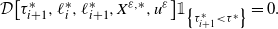 \begin{equation*}\mathcal{D}\big[\tau^{*}_{i+1},\ell^{*}_{i},\ell^{*}_{i+1},X^{\varepsilon,*}, u^{\varepsilon}\big]\unicode{x1D7D9}_{\big\{\tau^{*}_{i+1}<\tau^{*}\big\}}=0.\end{equation*}
Therefore, from here and (4.15), we obtain the desired result that was given in the lemma above.
4.2. Proof of Theorem 2.2
To conclude this section, we present the proof of Theorem 2.2, which will be proven under Assumptions (H1) and (H3)–(H5). Recall that
 $\mathcal{U}$
and
$\mathcal{U}$
and
 $\mathcal{S}$
are the families of controls
$\mathcal{S}$
are the families of controls
 $\xi=(\unicode{x1D55F},\zeta)$
and
$\xi=(\unicode{x1D55F},\zeta)$
and
 $\varsigma=(\tau_{i},\ell_{i})_{i\geq0}$
that satisfy (2.1) and (2.2), respectively. The functional cost
$\varsigma=(\tau_{i},\ell_{i})_{i\geq0}$
that satisfy (2.1) and (2.2), respectively. The functional cost
 $V_{\xi,\varsigma}$
is given by (1.2) for
$V_{\xi,\varsigma}$
is given by (1.2) for
 $(\xi,\varsigma)\in\mathcal{U}\times\mathcal{S}$
.
$(\xi,\varsigma)\in\mathcal{U}\times\mathcal{S}$
.
Proof of Theorem 2.2. Let
 $\{u^{\varepsilon_{n}}\}_{n\geq1}$
be the sequence of unique strong solutions to the HJB equation (2.20), when
$\{u^{\varepsilon_{n}}\}_{n\geq1}$
be the sequence of unique strong solutions to the HJB equation (2.20), when
 $\varepsilon=\varepsilon_{n}$
, which satisfy (3.27). From Lemma 4.3, we know that
$\varepsilon=\varepsilon_{n}$
, which satisfy (3.27). From Lemma 4.3, we know that
 \begin{equation*}u^{\varepsilon_{n}}_{\tilde{\ell}}(\tilde{x})=\mathcal{V}_{\xi^{\varepsilon_{n},*},\varsigma^{\varepsilon_{n},*}}\big(\tilde{x},\tilde{\ell}\big)= V^{\varepsilon_{n}}\big(\tilde{x},\tilde{\ell}\big)\quad\text{for $\big(\tilde{x},\tilde{\ell}\big)\in\overline{\mathcal{O}}\times\mathbb{I}$},\end{equation*}
with
 $(\xi^{\varepsilon_{n},*},\varsigma^{\varepsilon_{n},*})$
as in (4.7)–(4.10) and (4.12)–(4.13), when
$(\xi^{\varepsilon_{n},*},\varsigma^{\varepsilon_{n},*})$
as in (4.7)–(4.10) and (4.12)–(4.13), when
 $\varepsilon=\varepsilon_{n}$
. Notice that
$\varepsilon=\varepsilon_{n}$
. Notice that
 \begin{equation*}l_{\varepsilon_{n}}(x,\beta\gamma)\geq\big\langle\beta\gamma, g_{\ell^{*}_{i}} (x)\gamma\big\rangle-\psi_{\varepsilon_{n}}\big(| g_{\ell^{*}_{i}}(x)\gamma|^{2}- g_{\ell^{*}_{i}}(x)^{2}\big)=\beta g _{\ell^{*}_{i}} (x),\end{equation*}
with
 $\beta\in\mathbb{R}$
and
$\beta\in\mathbb{R}$
and
 $\gamma\in\mathbb{R}^{d}$
a unit vector. Then, from here and considering
$\gamma\in\mathbb{R}^{d}$
a unit vector. Then, from here and considering
 $(X^{\varepsilon_{n},*},I^{\varepsilon_{n},*})$
governed by (4.6) and (4.11), it follows that
$(X^{\varepsilon_{n},*},I^{\varepsilon_{n},*})$
governed by (4.6) and (4.11), it follows that
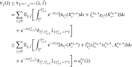
Notice that
 $V_{\xi^{\varepsilon_{n},*},\varsigma^{\varepsilon_{n},*}}$
is the cost function given in (1.2) corresponding to the control
$V_{\xi^{\varepsilon_{n},*},\varsigma^{\varepsilon_{n},*}}$
is the cost function given in (1.2) corresponding to the control
 $(\xi^{\varepsilon_{n},*},\varsigma^{\varepsilon_{n},*})$
where the second term in the right-hand side of (2.5) is zero, since
$(\xi^{\varepsilon_{n},*},\varsigma^{\varepsilon_{n},*})$
where the second term in the right-hand side of (2.5) is zero, since
 $\zeta^{\varepsilon_{n},*}$
has the continuous part only. Letting
$\zeta^{\varepsilon_{n},*}$
has the continuous part only. Letting
 $\varepsilon_{n}\rightarrow0$
in (4.16), we have
$\varepsilon_{n}\rightarrow0$
in (4.16), we have
 $u_{\tilde{\ell}}(\tilde{x})\geq V_{\tilde{\ell}}(\tilde{x})$
for each
$u_{\tilde{\ell}}(\tilde{x})\geq V_{\tilde{\ell}}(\tilde{x})$
for each
 $\big(\tilde{x},\tilde{\ell}\big)\in\overline{\mathcal{O}}\times\mathbb{I}$
.
$\big(\tilde{x},\tilde{\ell}\big)\in\overline{\mathcal{O}}\times\mathbb{I}$
.
Let
 $\big\{u^{\varepsilon_{n},\delta_{\hat{n}}}\big\}_{n,\hat{n}\geq1}$
be the sequence of unique solutions to the NPDS (3.1), when
$\big\{u^{\varepsilon_{n},\delta_{\hat{n}}}\big\}_{n,\hat{n}\geq1}$
be the sequence of unique solutions to the NPDS (3.1), when
 $\varepsilon=\varepsilon_{n}$
and
$\varepsilon=\varepsilon_{n}$
and
 $\delta=\delta_{\hat{n}}$
, which satisfy (3.5) and (3.27). Let us assume (X, I) evolves as in (1.1) with initial state
$\delta=\delta_{\hat{n}}$
, which satisfy (3.5) and (3.27). Let us assume (X, I) evolves as in (1.1) with initial state
 $\big(\tilde{x},\tilde{\ell}\big)\in\overline{\mathcal{O}}\times\mathbb{I}$
and the control process
$\big(\tilde{x},\tilde{\ell}\big)\in\overline{\mathcal{O}}\times\mathbb{I}$
and the control process
 $(\xi,\varsigma)$
belongs to
$(\xi,\varsigma)$
belongs to
 $\mathcal{U}\times\mathcal{S}$
. Take
$\mathcal{U}\times\mathcal{S}$
. Take ![]() , with
, with
 $i\geq1$
,
$i\geq1$
,
 $\mathcal{O}_{q}\,:\!=\,\{x\in\mathcal{O}\,:\,dist(x,\partial\mathcal{O} )>1/q\}$
, and q a positive integer large enough. Using integration by parts and Itô’s formula in
$\mathcal{O}_{q}\,:\!=\,\{x\in\mathcal{O}\,:\,dist(x,\partial\mathcal{O} )>1/q\}$
, and q a positive integer large enough. Using integration by parts and Itô’s formula in ![]() on
on
 $ \big[\hat{\tau}^{q}_{i},\hat{\tau}^{q}_{i+1}\big)$
,
$ \big[\hat{\tau}^{q}_{i},\hat{\tau}^{q}_{i+1}\big)$
,
 $i\geq0$
, we get that
$i\geq0$
, we get that

where ![]() is as in (4.2) and
is as in (4.2) and
Since ![]() for
for ![]() ,
,
 $i\geq0$
, and
$i\geq0$
, and
 $\mathcal{O}$
is a convex set, by the mean value theorem, we have
$\mathcal{O}$
is a convex set, by the mean value theorem, we have

Taking the expected value in (4.17), and since ![]() is a square-integrable martingale and
is a square-integrable martingale and
 $\big[c_{\ell_{i}}-\mathcal{L}_{\ell_{i}}\big]u^{\varepsilon_{n},\delta_{\hat{n}}}_{\ell_{i}}\leq h_{\ell_{i}}$
, we obtain
$\big[c_{\ell_{i}}-\mathcal{L}_{\ell_{i}}\big]u^{\varepsilon_{n},\delta_{\hat{n}}}_{\ell_{i}}\leq h_{\ell_{i}}$
, we obtain
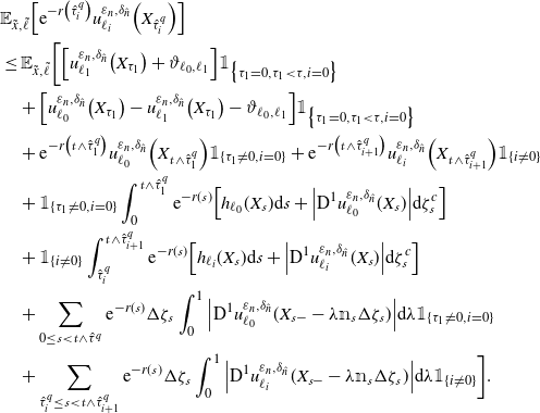
Notice that for ![]() ,
,

with
 $\lambda\in[0,1]$
. Then, letting
$\lambda\in[0,1]$
. Then, letting
 $\varepsilon_{n},\delta_{\hat{n}}\rightarrow0$
in (4.18), by the dominated convergence theorem and using
$\varepsilon_{n},\delta_{\hat{n}}\rightarrow0$
in (4.18), by the dominated convergence theorem and using
 $\big|\textrm{D}^{1} u_{\ell_{i}}\big|\leq g_{\ell_{i}}$
, we have
$\big|\textrm{D}^{1} u_{\ell_{i}}\big|\leq g_{\ell_{i}}$
, we have

with ![]() as in (2.5). Again, letting
as in (2.5). Again, letting
 $q\rightarrow\infty$
and
$q\rightarrow\infty$
and ![]() in (4.19), we have
in (4.19), we have

for
 $i\geq0$
, with
$i\geq0$
, with
 $\tilde{\tau}_{i}=\tau_{i}\wedge\tau$
and
$\tilde{\tau}_{i}=\tau_{i}\wedge\tau$
and
 $\mathcal{D}[\tau_{i+1},\ell_{i},\ell_{i+1},X, u ]$
as in (4.4). Noticing that
$\mathcal{D}[\tau_{i+1},\ell_{i},\ell_{i+1},X, u ]$
as in (4.4). Noticing that
 \begin{equation*}\mathcal{D}[\tau_{i+1},\ell_{i},\ell_{i+1},X, u ]\unicode{x1D7D9}_{\{\tau_{i+1}<\tau\}}\leq0\end{equation*}
and using (1.2), (4.20), we obtain
 $u_{\tilde{\ell}}(\tilde{x})\leq V_{\xi,\varsigma}\big(\tilde{x},\tilde{\ell}\big)$
for each
$u_{\tilde{\ell}}(\tilde{x})\leq V_{\xi,\varsigma}\big(\tilde{x},\tilde{\ell}\big)$
for each
 $\big(\tilde{x},\tilde{\ell}\big)\in\overline{\mathcal{O}}\times\mathbb{I}$
. Since the previous property is true for each control
$\big(\tilde{x},\tilde{\ell}\big)\in\overline{\mathcal{O}}\times\mathbb{I}$
. Since the previous property is true for each control
 $(\xi,\varsigma)\in\mathcal{U}\times\mathcal{S}$
, we conclude that
$(\xi,\varsigma)\in\mathcal{U}\times\mathcal{S}$
, we conclude that
 $u_{\tilde{\ell}}(\tilde{x})\leq V_{\tilde{\ell}}(\tilde{x})$
for each
$u_{\tilde{\ell}}(\tilde{x})\leq V_{\tilde{\ell}}(\tilde{x})$
for each
 $\big(\tilde{x},\tilde{\ell}\big)\in\overline{\mathcal{O}}\times\mathbb{I}$
.
$\big(\tilde{x},\tilde{\ell}\big)\in\overline{\mathcal{O}}\times\mathbb{I}$
.
4.3. On
$\varepsilon$
-PACS optimal controls

Previously, we checked that the value function
 $V_{ \ell}$
, defined in (2.8), satisfies the HJB equation (2.9). This means that for each
$V_{ \ell}$
, defined in (2.8), satisfies the HJB equation (2.9). This means that for each
 $\ell\in\mathbb{I}$
fixed, the domain set
$\ell\in\mathbb{I}$
fixed, the domain set
 $\mathcal{O}$
is divided into three parts. Consider
$\mathcal{O}$
is divided into three parts. Consider
 $\mathcal{C}_{\ell}\,:\!=\,\mathcal{O}\setminus(\mathcal{N}_{\ell}\cup \mathcal{S}_{\ell})$
where
$\mathcal{C}_{\ell}\,:\!=\,\mathcal{O}\setminus(\mathcal{N}_{\ell}\cup \mathcal{S}_{\ell})$
where
 \begin{equation*}\mathcal{N}_{\ell}\,:\!=\,\big\{x\in\mathcal{O}\,:\,|\textrm{D}^{1}V_{\ell}|= g_{\ell}\big\}\quad \text{and} \quad \mathcal{S}_{\ell}=\{x\in\mathcal{O}\,:\,V_{\ell}=\mathcal{M}_{\ell}V\}.\end{equation*}
The open set
 $\mathcal{C}_{\ell}$
is where
$\mathcal{C}_{\ell}$
is where
 $V_{\ell}$
satisfies the elliptic partial differential equation
$V_{\ell}$
satisfies the elliptic partial differential equation
 $[c_{\ell}-\mathcal{L}_{\ell}] V_{\ell}=h_{\ell}$
, which suggests that the ‘optimal control’
$[c_{\ell}-\mathcal{L}_{\ell}] V_{\ell}=h_{\ell}$
, which suggests that the ‘optimal control’
 $(\xi^{*},\varsigma^{*})$
corresponding to this problem will not be exercised when the process
$(\xi^{*},\varsigma^{*})$
corresponding to this problem will not be exercised when the process
 $X^{\xi^{*},\varsigma^{*}}$
is in
$X^{\xi^{*},\varsigma^{*}}$
is in
 $\mathcal{C}_{\ell}$
. Otherwise, either
$\mathcal{C}_{\ell}$
. Otherwise, either
 $\xi^{*}$
or
$\xi^{*}$
or
 $\varsigma^{*}$
will be exercised on
$\varsigma^{*}$
will be exercised on
 $X^{\xi^{*},\varsigma^{*}}$
in the following way:
$X^{\xi^{*},\varsigma^{*}}$
in the following way:
-
(i) if
$X^{\xi^{*},\varsigma^{*}}\in\mathcal{N}_{\ell}\setminus\mathcal{S}_{\ell}$
, the singular control
$\xi^{*}$
will act on
$X^{\xi^{*},\varsigma^{*}}$
in such a way that
$ X^{\xi^{*},\varsigma^{*}} $
will be pushed back to some point
$y \in\partial\mathcal{C}_{\ell}$
; -
(ii) if
$X^{\xi^{*},\varsigma^{*}}\in \mathcal{S}_{\ell}$
, the switching control
$\varsigma^{*}$
will be executed in such a way that the process
$ X^{\xi^{*},\varsigma^{*}} $
will switch to some regime
$\kappa\neq\ell$
at time
$\tau_{\kappa}\leq\tau$
.


The construction of an optimal strategy for the problem (2.8) still remains an open problem of interest. A way to carry out this construction is to verify first that
 $\partial\mathcal{C}_{\ell}$
is at least of class
$\partial\mathcal{C}_{\ell}$
is at least of class
 $\text{C}^{1}$
, which is not easy to do.
$\text{C}^{1}$
, which is not easy to do.
In the literature, we can see that the existence of an optimal dividend/switching strategy, which is an example of a mixed singular/switching control problem, has been solved when the payoff expected value is given by (1.4) and the cash reserve process switches between m-regimes governed by different Poisson processes with drifts; see [Reference Azcue and Muler2], in which the authors proved that their solution is stationary with a band structure.
Another way to address the problem (2.8) is by means of
 $\varepsilon$
-PACS optimal controls, which have been constructed in (4.6)–(4.13).
$\varepsilon$
-PACS optimal controls, which have been constructed in (4.6)–(4.13).
By Lemma 4.3 and the proof of Theorem 2.2, it is known that for each
 $\ell\in\mathbb{I}$
,
$\ell\in\mathbb{I}$
,
 $V^{\varepsilon_{n}}_{\ell}\rightarrow V_{\ell}$
as
$V^{\varepsilon_{n}}_{\ell}\rightarrow V_{\ell}$
as
 $\varepsilon_{n}\downarrow0$
, and
$\varepsilon_{n}\downarrow0$
, and
 $V_{\ell}\leq V_{\xi^{\varepsilon_{n},*},\varsigma^{\varepsilon_{n},*}}(\cdot, \ell)\leq V^{\varepsilon_{n}}_{\ell}\ \text{on} \overline{\mathcal{O}}$
, with
$V_{\ell}\leq V_{\xi^{\varepsilon_{n},*},\varsigma^{\varepsilon_{n},*}}(\cdot, \ell)\leq V^{\varepsilon_{n}}_{\ell}\ \text{on} \overline{\mathcal{O}}$
, with
 $\big(\xi^{\varepsilon_{n},*},\varsigma^{\varepsilon_{n},*}\big)$
as in (4.6)–(4.13), and
$\big(\xi^{\varepsilon_{n},*},\varsigma^{\varepsilon_{n},*}\big)$
as in (4.6)–(4.13), and
 $V_{\xi^{\varepsilon_{n},*},\varsigma^{\varepsilon_{n},*}}(\cdot,\ell),V_{\ell}, V^{\varepsilon_{n}}_{\ell}$
given by (1.2), (2.8), and (2.18), respectively.
$V_{\xi^{\varepsilon_{n},*},\varsigma^{\varepsilon_{n},*}}(\cdot,\ell),V_{\ell}, V^{\varepsilon_{n}}_{\ell}$
given by (1.2), (2.8), and (2.18), respectively.
Taking
 $\varepsilon_{n}$
small enough and assuming that the process
$\varepsilon_{n}$
small enough and assuming that the process ![]() is on the regime
is on the regime
 $\ell^{*}_{i}$
at time
$\ell^{*}_{i}$
at time ![]() , we have that
, we have that ![]() and the control
and the control
 $\big(\xi^{\varepsilon_{n},*},\varsigma^{\varepsilon_{n},*}\big)$
will be exercised as follows:
$\big(\xi^{\varepsilon_{n},*},\varsigma^{\varepsilon_{n},*}\big)$
will be exercised as follows:
-
(i) if the controlled process
$X^{ \varepsilon_{n},*}$
satisfies then and will stay in
$\mathcal{C}_{\ell_{i}^{*}}$
;
-
(ii) if
, the process will be crossing
$\partial\mathcal{C}_{\ell_{i}^{*}}$
persistently; -
(iii) otherwise,
will exercise a force and in the directionat in such a way that it will be pushed back to
$\partial\mathcal{C}_{\ell_{i}^{*}}$
.
-
(iv) At time
,
$X^{\varepsilon_{n},*}_{\tau_{i+1}^{*}}$
will be in
$\mathcal{S}^{\varepsilon_{n}}_{\ell_{i}^{*}}$
for the first time and will switch to the regime
$\ell_{i+1}^{*}$
.


This procedure will be repeated until the time
 $\tau^{*}$
, which represents the first exit time of the process
$\tau^{*}$
, which represents the first exit time of the process
 $X^{\varepsilon_{n},*}$
from the set
$X^{\varepsilon_{n},*}$
from the set
 $\mathcal{O}$
.
$\mathcal{O}$
.
5. Explicit solution to the HJB equation (2.9) on open intervals of
$\mathbb{R}$

In this section, we consider the controlled process
 $\big(X^{\xi,\varsigma},I^{\varsigma}\big)$
that evolves as (1.1) where
$\big(X^{\xi,\varsigma},I^{\varsigma}\big)$
that evolves as (1.1) where
 $X^{\xi,\varsigma}_{0}=\tilde{x}\in(0,l)\subset\mathbb{R}$
, for some
$X^{\xi,\varsigma}_{0}=\tilde{x}\in(0,l)\subset\mathbb{R}$
, for some
 $l>0$
fixed, and
$l>0$
fixed, and
 $I^{\varsigma}_{0-}=\tilde{\ell}\in\mathbb{I}\,:\!=\,\{1,\dots,m\}$
. Here
$I^{\varsigma}_{0-}=\tilde{\ell}\in\mathbb{I}\,:\!=\,\{1,\dots,m\}$
. Here
 $W=\{W_{t}\,:\,t\geq0\}$
is a one-dimensional standard Brownian motion. The parameters of the SDE (1.1) are given by
$W=\{W_{t}\,:\,t\geq0\}$
is a one-dimensional standard Brownian motion. The parameters of the SDE (1.1) are given by
 $b(x,\ell)=b_{\ell}x$
and
$b(x,\ell)=b_{\ell}x$
and
 $\sigma(x,\ell)=\sigma_{\ell}x$
for
$\sigma(x,\ell)=\sigma_{\ell}x$
for
 $x\in(0,l)$
, with
$x\in(0,l)$
, with
 $b_{\ell},\sigma_{\ell}\in\mathbb{R}$
such that
$b_{\ell},\sigma_{\ell}\in\mathbb{R}$
such that
 $\sigma_{\ell}>0$
.
$\sigma_{\ell}>0$
.
Let us take the value function
 $V_{\tilde{\ell}}(\tilde{x})$
as in (1.3) where
$V_{\tilde{\ell}}(\tilde{x})$
as in (1.3) where
 $c_{\ell}(x)$
and
$c_{\ell}(x)$
and
 $g_{\ell}(x)$
are positive constant functions that are denoted by
$g_{\ell}(x)$
are positive constant functions that are denoted by
 $c_{\ell}$
and
$c_{\ell}$
and
 $ g_{\ell}$
, respectively, and the running cost
$ g_{\ell}$
, respectively, and the running cost
 $h_{\ell}$
is taken as
$h_{\ell}$
is taken as
 $h_{\ell}(x)\,:\!=\, K_{\ell}x^{\gamma_{\ell}}$
where
$h_{\ell}(x)\,:\!=\, K_{\ell}x^{\gamma_{\ell}}$
where
 $\gamma_{\ell}\in(0,1)$
,
$\gamma_{\ell}\in(0,1)$
,
 $K_{\ell}>0$
are fixed. For simplicity, we assume that
$K_{\ell}>0$
are fixed. For simplicity, we assume that
 $\gamma_l\not=r_{2,l}$
; cf. (5.3). By Theorem 2.2, it is known that
$\gamma_l\not=r_{2,l}$
; cf. (5.3). By Theorem 2.2, it is known that
 $V_{\tilde{\ell}}(\tilde{x})$
satisfies (in the a.e. sense) the following HJB equation:
$V_{\tilde{\ell}}(\tilde{x})$
satisfies (in the a.e. sense) the following HJB equation:
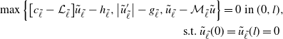 \begin{align}\max\Big\{\big[c_{\tilde{\ell}}-\mathcal{L}_{\tilde{\ell}}\big]\tilde{u}_{\tilde{\ell}}- h_{\tilde{\ell}},\big|\tilde{u}^{\prime}_{\tilde{\ell}}\big|- g_{\tilde{\ell}},\tilde{u}_{\tilde{\ell}}-\mathcal{M}_{\tilde{\ell}}\tilde{u}\Big\}= 0 \ \text{in}\ (0,l)&,\\\text{s.t.}\ \tilde{u}_{\tilde{\ell}}(0)=\tilde{u}_{\tilde{\ell}}(l)=0& \end{align}
where
 $\mathcal{M}_{\ell}\tilde{u}=\min_{\kappa\in \mathbb{I}\setminus\{\ell\}}\{\tilde{u}_{\kappa}+\vartheta_{\ell,\kappa}\}$
, and the parameters
$\mathcal{M}_{\ell}\tilde{u}=\min_{\kappa\in \mathbb{I}\setminus\{\ell\}}\{\tilde{u}_{\kappa}+\vartheta_{\ell,\kappa}\}$
, and the parameters
 $\vartheta_{{\ell},\kappa}\in \mathbb{R}$
are nonnegative and satisfy (2.6)–(2.7). Here
$\vartheta_{{\ell},\kappa}\in \mathbb{R}$
are nonnegative and satisfy (2.6)–(2.7). Here
 \begin{equation*}\mathcal{L}_{{\ell}}\tilde{u}_{\ell}(x)=\dfrac{1}{2}\sigma_{\ell}^{2}x^{2}\tilde{u}^{\prime\prime}_{\ell}(x)-b_{\ell}x\tilde{u}^{\prime}_{\ell},\end{equation*}
and
 $\tilde{u}_{\ell}^{\prime}$
,
$\tilde{u}_{\ell}^{\prime}$
,
 $\tilde{u}_{\ell}^{\prime\prime}$
represent the first and second derivatives of
$\tilde{u}_{\ell}^{\prime\prime}$
represent the first and second derivatives of
 $\tilde{u}_{\ell}$
.
$\tilde{u}_{\ell}$
.
In the subsection below, we shall give an explicit solution to the HJB equation (5.1) with some additional restrictions on the constant parameters.
5.1. Construction of the solution to the HJB equation (5.1)
Considering
 $\ell\in\mathbb{I}$
fixed, let us first construct the solution to the following system of variational inequalities:
$\ell\in\mathbb{I}$
fixed, let us first construct the solution to the following system of variational inequalities:
 \begin{align}&\max\Big\{\big[c_{{\ell}}-\mathcal{L}_{{\ell}}\big]\tilde{u}_{{\ell}}- h_{{\ell}},\big|\tilde{u}^{\prime}_{{\ell}}\big|- g_{{\ell}}\Big\}= 0\ \text{in}\ (0,l),\quad\text{s.t.}\ \tilde{u}_{{\ell}}(0)=\tilde{u}_{{\ell}}(l)=0.\end{align}
It is well known that the general solution to
 $[c_{\ell} -\mathcal{L}_{\ell}] \tilde{u}_{\ell}=h_\ell$
on
$[c_{\ell} -\mathcal{L}_{\ell}] \tilde{u}_{\ell}=h_\ell$
on
 $\big[x^{*}_{\ell},l\big]$
, with
$\big[x^{*}_{\ell},l\big]$
, with
 $x^{*}_{\ell}>0$
, has the form
$x^{*}_{\ell}>0$
, has the form
 \begin{equation*}\tilde{u}_{\ell}(x)=A_{\ell}x^{r_{1,\ell}}+B_{\ell}x^{r_{2,\ell}}+\overline{K}_{\ell}x^{\gamma_{\ell}},\end{equation*}
where
 \begin{equation*}\overline{K}_{\ell}=\frac{2 K_{\ell}}{\sigma^{2}(r_{1,\ell}-\gamma_{\ell})(\gamma_{\ell}-r_{2,\ell})}\end{equation*}
and
 $ r_{1,\ell},r_{2,\ell}$
denote the negative and positive solutions to
$ r_{1,\ell},r_{2,\ell}$
denote the negative and positive solutions to
 \begin{equation}r^{2}-\bigg(\dfrac{2b_{\ell}}{\sigma^{2}_{\ell}}+1\bigg)r-\dfrac{2c_{\ell}}{\sigma^{2}_{\ell}}=0.\end{equation}
Taking
 \begin{equation}\tilde{u}_{\ell}(x)\,:\!=\,\begin{cases}g_{\ell}x&\text{if}\ 0\leq x<x^{*}_{\ell},\\[3pt]A_{\ell}x^{r_{1,\ell}}+B_{\ell}x^{r_{2,\ell}}+\overline{K}_{\ell}x^{\gamma_{\ell}} &\text{if}\ x^{*}_{\ell}\leq x\leq l,\end{cases}\end{equation}
we see easily that
 \begin{equation*}\big|\tilde{u}^{\prime}_\ell\big|-g_{\ell}=0\ \text{on}\ \big[0,x^{*}_{\ell}\big)\quad\text{and}\quad [c_{\ell}-\mathcal{L}_{\ell}] \tilde{u}_{\ell}-h_{\ell}=0\ \text{on}\ \big[x^{*}_{\ell},l\big],\end{equation*}
and if
 $c_{\ell}+b_{\ell}\leq0$
, then
$c_{\ell}+b_{\ell}\leq0$
, then
 \begin{equation*}[c_{\ell}-\mathcal{L}_{\ell}] \tilde{u}_{\ell}(x)-h_{\ell}(x)=g_{\ell}(c_{\ell}+b_{\ell})x-K_{\ell}x^{\gamma_{\ell}}<0\quad \text{for}\ x\in\big(0,x^{*}_{\ell}\big).\end{equation*}
In order for
 $\tilde{u}$
to satisfy (5.2), we shall consider parameters
$\tilde{u}$
to satisfy (5.2), we shall consider parameters
 $b_{\ell}$
,
$b_{\ell}$
,
 $\sigma_{\ell}$
,
$\sigma_{\ell}$
,
 $c_{\ell}$
, and
$c_{\ell}$
, and
 $g_{\ell}$
such that
$g_{\ell}$
such that
 \begin{equation}\big|u^{\prime}_{\ell}\big|-g_{\ell}\leq0\quad\text{on}\ \big(x^{*}_{\ell},l\big).\end{equation}
Additionally, they must satisfy
 \begin{equation}x^{*}_{\ell}<\bigg(\dfrac{K_{\ell}}{g_{\ell}(c_{\ell}+b_{\ell})}\bigg)^{\frac{1}{1-\gamma_{\ell}}},\quad\text{if}\ c_{\ell}+b_{\ell}>0,\end{equation}
since if (5.6) holds and
 $x\in\big(0,x^{*}_{\ell}\big)$
, then
$x\in\big(0,x^{*}_{\ell}\big)$
, then
 \begin{align}[c_{\ell}-\mathcal{L}_{\ell}] \tilde{u}_{\ell}(x)-h_{\ell}(x)&=x^{\gamma_{\ell}}\big(g_{\ell}(c_{\ell}+b_{\ell})x^{1-\gamma_{\ell}}-K_{\ell}\big)\notag\\&<x^{\gamma_{\ell}}\big(g_{\ell}(c_{\ell}+b_{\ell})\big(x^{*}_{\ell}\big)^{1-\gamma_{\ell}}-K_{\ell}\big)<0.\end{align}
In order for
 $\tilde{u}_{\ell}$
to belong to
$\tilde{u}_{\ell}$
to belong to
 $\text{C}^{1}([0,l])$
, by smooth fit, the parameters
$\text{C}^{1}([0,l])$
, by smooth fit, the parameters
 $A_{\ell}$
,
$A_{\ell}$
,
 $B_{\ell}$
, and
$B_{\ell}$
, and
 $x^{*}_{\ell}$
must satisfy the following system of equations:
$x^{*}_{\ell}$
must satisfy the following system of equations:
 \begin{align}&A_{\ell}l^{r_{1,\ell}}+B_{\ell}l^{r_{2,\ell}}+\overline{K}_{\ell}l^{\gamma_{\ell}}=0, \\&A_{\ell}+B_{\ell}\big(x^{*}_{\ell}\big)^{r_{2,\ell}-r_{1,\ell}}+\overline{K}\big(x^{*}_{\ell}\big)^{\gamma_{\ell}-r_{1,\ell}}-g_{\ell}\big(x^{*}_{\ell}\big)^{1-r_{1,\ell}}=0,\\&r_{1,\ell}A_{\ell}+r_{2,\ell}B_{\ell}\big(x^{*}_{\ell}\big)^{r_{2,\ell}-r_{1,\ell}}+\gamma_{\ell}\overline{K}_{\ell} \big(x^{*}_{\ell}\big)^{\gamma_{\ell}-r_{1,\ell}}-g_{\ell}\big(x^{*}_{\ell}\big)^{1-r_{1,\ell}}=0,\quad\text{s.t.}\ (5.6).\end{align}
By what we have seen previously, we have the next result.
Proposition 5.1. Let
 $b_{\ell}$
,
$b_{\ell}$
,
 $\sigma_{\ell}$
,
$\sigma_{\ell}$
,
 $c_{\ell}$
, and
$c_{\ell}$
, and
 $g_{\ell}$
be parameters satisfying (5.5) and (5.6). Then the function
$g_{\ell}$
be parameters satisfying (5.5) and (5.6). Then the function
 $\tilde{u}_{\ell}$
given as in (5.4) is a solution to the variational inequalities (5.2). Moreover, if
$\tilde{u}_{\ell}$
given as in (5.4) is a solution to the variational inequalities (5.2). Moreover, if
 $A_{\ell}$
,
$A_{\ell}$
,
 $B_{\ell}$
, and
$B_{\ell}$
, and
 $x^{*}_{\ell}$
are a solution to (5.8), then
$x^{*}_{\ell}$
are a solution to (5.8), then
 $\tilde{u}_{\ell}$
belongs to
$\tilde{u}_{\ell}$
belongs to
 $\text{C}^{1}([0,l])\cap \text{C}^{2}\big([0,l]\setminus\big\{x^{*}_{\ell}\big\}\big)$
and is unique in this space.
$\text{C}^{1}([0,l])\cap \text{C}^{2}\big([0,l]\setminus\big\{x^{*}_{\ell}\big\}\big)$
and is unique in this space.
The uniqueness of
 $\tilde{u}_{\ell}$
is guaranteed by [Reference Evans7, Theorem 1.1].
$\tilde{u}_{\ell}$
is guaranteed by [Reference Evans7, Theorem 1.1].
Numerical examples. Table 1 contains the values that are considered to find numerically the solution
 $\tilde{u}_{\ell}$
to the variational inequalities (5.2), when
$\tilde{u}_{\ell}$
to the variational inequalities (5.2), when
 $\ell=1,2,3$
and
$\ell=1,2,3$
and
 $l=3$
; see the left panel of Figure 1.
$l=3$
; see the left panel of Figure 1.


Table 2 presents the numerical solutions to the system of equations (5.3) and (5.8) for the parameters given in Table 1. Observe that when
 $\ell=2,3$
, the condition (5.6) is satisfied. The left panel of Figure 3 shows that (5.5) and (5.7) are satisfied for the parameters seen in Table 1. From here observe that
$\ell=2,3$
, the condition (5.6) is satisfied. The left panel of Figure 3 shows that (5.5) and (5.7) are satisfied for the parameters seen in Table 1. From here observe that
 $\tilde{u}$
is the numerical solution to the variational inequality (5.2) for the parameters given in Table 1.
$\tilde{u}$
is the numerical solution to the variational inequality (5.2) for the parameters given in Table 1.
Table 2. Approximate solution to the system of equations (5.3) and (5.8) with the parameters given in Table 1.
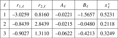

Let us now give two examples where the conditions (5.5) and (5.6) are not satisfied. Consider the following parameters:
Table 4 presents the numerical solutions to the system of equations (5.3) and (5.8). The left panel of Figure 2 shows that
 $\tilde{u}_{1}$
does not satisfy the condition (5.5). Notice that
$\tilde{u}_{1}$
does not satisfy the condition (5.5). Notice that
 $x^{*}_{2}\approx 0.4411 $
does not satisfy the condition (5.6), leaving a discontinuity of
$x^{*}_{2}\approx 0.4411 $
does not satisfy the condition (5.6), leaving a discontinuity of
 $\tilde{u}_{2}$
at
$\tilde{u}_{2}$
at
 $x^{*}_{2}$
; see the right panel of Figure 1. Additionally, in the right panel of Figure 2, we see that
$x^{*}_{2}$
; see the right panel of Figure 1. Additionally, in the right panel of Figure 2, we see that
 $\tilde{u}_{2}$
violates (5.7).
$\tilde{u}_{2}$
violates (5.7).
Table 4. Approximate solution to the system of equations (5.3) and (5.8) for the parameters given in Table 3.
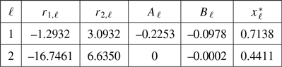
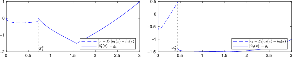
Figure 2. The left and right panels show plots of
 $[c_{\ell}-\mathcal{L}_{\ell}]\tilde{u}_{\ell}-h_{\ell}$
and
$[c_{\ell}-\mathcal{L}_{\ell}]\tilde{u}_{\ell}-h_{\ell}$
and
 $\big|\tilde{u}^{\prime}_{\ell}\big|-g_{\ell}$
on
$\big|\tilde{u}^{\prime}_{\ell}\big|-g_{\ell}$
on
 $\big(0,x^{*}_{\ell}\big)$
and
$\big(0,x^{*}_{\ell}\big)$
and
 $\big(x^{*}_{\ell}, l\big)$
for the parameters given in Table 4.
$\big(x^{*}_{\ell}, l\big)$
for the parameters given in Table 4.
5.1.1. Construction of the solution to (5.1)
In this part, we consider the vector function
 $\tilde{u}=\big(\tilde{u}_{1},\dots,\tilde{u}_{m}\big)$
such that its elements are given as (5.4) and satisfy the hypothesis of Proposition 5.1 in such a way that
$\tilde{u}=\big(\tilde{u}_{1},\dots,\tilde{u}_{m}\big)$
such that its elements are given as (5.4) and satisfy the hypothesis of Proposition 5.1 in such a way that
 $\tilde{u}_{\ell}$
belongs to
$\tilde{u}_{\ell}$
belongs to
 $\textrm{C}^{1}([0,l])\cap \textrm{C}^{2}\big([0,l]\setminus\{x^{*}_{\ell}\}\big)$
and is the unique solution of (5.2) for each
$\textrm{C}^{1}([0,l])\cap \textrm{C}^{2}\big([0,l]\setminus\{x^{*}_{\ell}\}\big)$
and is the unique solution of (5.2) for each
 $\ell\in\mathbb{I}$
. Assume that the entrances of
$\ell\in\mathbb{I}$
. Assume that the entrances of
 $\tilde{u}$
are different.
$\tilde{u}$
are different.
We will study the parameters
 $\vartheta_{\ell,\kappa}\geq0$
where
$\vartheta_{\ell,\kappa}\geq0$
where
 $\tilde{u}$
satisfies the HJB equation (5.1). For that, define first the sets
$\tilde{u}$
satisfies the HJB equation (5.1). For that, define first the sets
 $\mathcal{D}_{\ell,\kappa}$
and
$\mathcal{D}_{\ell,\kappa}$
and
 $\mathcal{U}_{\ell,\kappa}$
, with
$\mathcal{U}_{\ell,\kappa}$
, with
 $\ell\neq\kappa$
, by
$\ell\neq\kappa$
, by
 \begin{align*}\mathcal{D}_{\ell,\kappa}&=\big\{x\in(0,l)\,:\, u^{\prime}_{\ell}(x)= u^{\prime}_{\kappa}(x)\big\},\\{\mathcal{U}}_{\ell,\kappa}&=\big\{x\in\mathcal{D}_{\ell,\kappa}\,:\, 0\leq\big[\tilde{u}_{\ell}-\tilde{u}_{\kappa}\big](y)\leq\big[\tilde{u}_{\ell}-\tilde{u}_{\kappa}\big](x)\ \text{for any}\ y\in\mathcal{D}_{\ell,\kappa} \big\}.\end{align*}
Now let us take
 $\hat{\vartheta}_{\ell,\kappa}$
, with
$\hat{\vartheta}_{\ell,\kappa}$
, with
 $\ell,\kappa\in\mathbb{I}$
and
$\ell,\kappa\in\mathbb{I}$
and
 $\ell\neq\kappa$
, in the following way:
$\ell\neq\kappa$
, in the following way:
 \begin{equation}\hat{\vartheta}_{\ell,\kappa}\,:\!=\,\big[\tilde{u}_{\ell}-\tilde{u}_{\kappa}\big]\big(\bar{x}_{\ell,\kappa}\big),\quad\text{for some $\bar{x}_{\ell,\kappa}\in \mathcal{U}_{\ell,\kappa}$ fixed.}\end{equation}
If
 $ \mathcal{U}_{\ell,\kappa}=\emptyset$
, we set
$ \mathcal{U}_{\ell,\kappa}=\emptyset$
, we set
 $\hat{\vartheta}_{\ell,\kappa}=0$
. We have the following result.
$\hat{\vartheta}_{\ell,\kappa}=0$
. We have the following result.
Lemma 5.1. If
 $\tilde{u}_{\ell}<\tilde{u}_{\kappa}+\hat{\vartheta}_{\ell,\kappa}$
on
$\tilde{u}_{\ell}<\tilde{u}_{\kappa}+\hat{\vartheta}_{\ell,\kappa}$
on
 $(0,l)\setminus \mathcal{U}_{\ell,\kappa}$
, then
$(0,l)\setminus \mathcal{U}_{\ell,\kappa}$
, then
 $\tilde{u}_{\ell}$
is a solution to the following system of variational inequalities:
$\tilde{u}_{\ell}$
is a solution to the following system of variational inequalities:
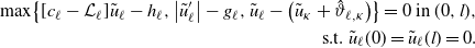 \begin{align} \max\!\big\{[c_{{\ell}}-\mathcal{L}_{{\ell}}]\tilde{u}_{{\ell}}- h_{{\ell}},\big|\tilde{u}^{\prime}_{{\ell}}\big|- g_{{\ell}},\tilde{u}_{\ell}-\big(\tilde{u}_{\kappa}+\hat{\vartheta}_{\ell,\kappa}\big)\big\}= 0 \ \text{in}\ (0,l),&\\\text{s.t.}\ \tilde{u}_{{\ell}}(0)=\tilde{u}_{{\ell}}(l)=0.& \end{align}
Remark 5.1. Notice that if
 $\vartheta_{\ell,\kappa}>\hat{\vartheta}_{\ell,\kappa}$
,
$\vartheta_{\ell,\kappa}>\hat{\vartheta}_{\ell,\kappa}$
,
 $\tilde{u}_{\ell}$
satisfies (5.10) with
$\tilde{u}_{\ell}$
satisfies (5.10) with
 $\hat{\vartheta}_{\ell,\kappa}$
replaced by
$\hat{\vartheta}_{\ell,\kappa}$
replaced by
 $\vartheta_{\ell,\kappa}$
, but there would be no opportunity to switch from the state
$\vartheta_{\ell,\kappa}$
, but there would be no opportunity to switch from the state
 $\ell$
to
$\ell$
to
 $\kappa$
since
$\kappa$
since
 $\tilde{u}_{\ell}<\tilde{u}_{\kappa}+ {\vartheta}_{\ell,\kappa}$
on (0,l).
$\tilde{u}_{\ell}<\tilde{u}_{\kappa}+ {\vartheta}_{\ell,\kappa}$
on (0,l).
To conclude this part, let us suppose that for each
 $\ell\in\mathbb{I}$
fixed,
$\ell\in\mathbb{I}$
fixed,
 $\tilde{u}_{\ell}$
satisfies the following condition:
$\tilde{u}_{\ell}$
satisfies the following condition:
 \begin{equation} \tilde{u}_{\ell}<\tilde{u}_{\kappa}+\hat{\vartheta}_{\ell,\kappa}\quad \text{on}\ (0,l)\setminus \mathcal{U}_{\ell,\kappa}\ \text{for each}\ \kappa\neq\ell. \end{equation}
From here, it is easy to see that
 \begin{equation*} \tilde{u}_{{\ell}}-\mathcal{M}_{{\ell}}\tilde{u}=\tilde{u}_{\ell}-\min_{\kappa\neq\ell}\big\{\tilde{u}_{\kappa}+\hat{\vartheta}_{\ell,\kappa}\big\}< 0\quad \text{on}\ (0,l)\setminus\bigcup_{\kappa\neq\ell}\mathcal{U}_{\ell,\kappa}. \end{equation*}
Remark 5.2. Defining
 $\widetilde{\mathcal{S}}_{\ell}=\{x\in(0,l)\,:\,\tilde{u}_{\ell}=\mathcal{M}_{\ell}\tilde{u}\}$
, we have that
$\widetilde{\mathcal{S}}_{\ell}=\{x\in(0,l)\,:\,\tilde{u}_{\ell}=\mathcal{M}_{\ell}\tilde{u}\}$
, we have that
 \begin{equation*} \widetilde{\mathcal{S}}_{\ell}=\bigcup_{\kappa\neq\ell}\mathcal{U}_{\ell,\kappa}\quad\text{for}\ \ell\in\mathbb{I}, \end{equation*}
which is the zone where it is optimal to switch from the state
 $\ell$
to some other state
$\ell$
to some other state
 $\kappa$
.
$\kappa$
.
Proposition 5.2. Let
 $\tilde{u}=\big(\tilde{u}_{1},\dots,\tilde{u}_{m}\big)$
be the vector function whose entrances, given by (5.4), are different and satisfy the hypotheses of Proposition 5.1 and the condition (5.11). If
$\tilde{u}=\big(\tilde{u}_{1},\dots,\tilde{u}_{m}\big)$
be the vector function whose entrances, given by (5.4), are different and satisfy the hypotheses of Proposition 5.1 and the condition (5.11). If
 $\hat{\vartheta}_{\ell,\kappa}$
, defined in (5.9), satisfy the conditions (2.6)–(2.7), then
$\hat{\vartheta}_{\ell,\kappa}$
, defined in (5.9), satisfy the conditions (2.6)–(2.7), then
 $\tilde{u}$
is the unique solution to (5.1).
$\tilde{u}$
is the unique solution to (5.1).
Remark 5.3. Taking
 $\widetilde{\mathcal{N}}_{\ell}\,:\!=\,\{x\in(0,l)\,:\,\big|\tilde{u}^{\prime}_{\ell}\big|-g_{\ell}=0\}$
, we have that
$\widetilde{\mathcal{N}}_{\ell}\,:\!=\,\{x\in(0,l)\,:\,\big|\tilde{u}^{\prime}_{\ell}\big|-g_{\ell}=0\}$
, we have that
 $\widetilde{\mathcal{C}}_{\ell}\,:\!=\,(0,l)\setminus(\widetilde{\mathcal{N}}_{\ell}\cup\widetilde{\mathcal{S}}_{\ell})$
is the zone where it is not optimal to switch to any other state.
$\widetilde{\mathcal{C}}_{\ell}\,:\!=\,(0,l)\setminus(\widetilde{\mathcal{N}}_{\ell}\cup\widetilde{\mathcal{S}}_{\ell})$
is the zone where it is not optimal to switch to any other state.
Numerical example. Consider the parameters given in Table 1. The left panel of Table 5 presents the approximate values of
 $\hat{\vartheta}_{\ell,\kappa}$
which are found using (5.9).
$\hat{\vartheta}_{\ell,\kappa}$
which are found using (5.9).
Table 5. The table on the left presents the approximate values of
 $\hat{\vartheta}_{\ell,\kappa}$
. The table on the right presents the approximate values of
$\hat{\vartheta}_{\ell,\kappa}$
. The table on the right presents the approximate values of
 $\hat{\vartheta}_{\ell,\bar{\kappa}}+\hat{\vartheta}_{\bar{\kappa},\kappa}$
, with
$\hat{\vartheta}_{\ell,\bar{\kappa}}+\hat{\vartheta}_{\bar{\kappa},\kappa}$
, with
 $\ell\neq\kappa\neq\bar{\kappa}$
.
$\ell\neq\kappa\neq\bar{\kappa}$
.
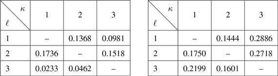
The right panel of Table 5 presents the approximate values of
 $\hat{\vartheta}_{\ell,\bar{\kappa}}+\hat{\vartheta}_{\bar{\kappa},\kappa}$
. Note that the inequalities (2.6)–(2.7) are always satisfied, say
$\hat{\vartheta}_{\ell,\bar{\kappa}}+\hat{\vartheta}_{\bar{\kappa},\kappa}$
. Note that the inequalities (2.6)–(2.7) are always satisfied, say
 $\hat{\vartheta}_{1,2}\approx0.1368<\hat{\vartheta}_{1,3}+\hat{\vartheta}_{3,2}\approx0.1444$
. Table 6 presents the approximate values of
$\hat{\vartheta}_{1,2}\approx0.1368<\hat{\vartheta}_{1,3}+\hat{\vartheta}_{3,2}\approx0.1444$
. Table 6 presents the approximate values of
 $\bar{x}_{\ell,\kappa}$
where switching from the state
$\bar{x}_{\ell,\kappa}$
where switching from the state
 $\ell$
to the state
$\ell$
to the state
 $\kappa$
is recommended.
$\kappa$
is recommended.
Table 6. Approximate values of
 $\bar{x}_{\ell,\kappa}$
where switching from the state
$\bar{x}_{\ell,\kappa}$
where switching from the state
 $\ell$
to the state
$\ell$
to the state
 $\kappa$
is recommended.
$\kappa$
is recommended.
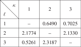
Finally, Figure 3 shows that the function
 $\tilde{u}_{\ell}$
indeed satisfies the HJB equation (5.1). The figures in the left column show the plots of
$\tilde{u}_{\ell}$
indeed satisfies the HJB equation (5.1). The figures in the left column show the plots of
 $[c_{\ell}-\mathcal{L}_{\ell}]\tilde{u}_{\ell}-h_{\ell}$
and
$[c_{\ell}-\mathcal{L}_{\ell}]\tilde{u}_{\ell}-h_{\ell}$
and
 $\big|\tilde{u}^{\prime}_{\ell}\big|-g_{\ell}$
on
$\big|\tilde{u}^{\prime}_{\ell}\big|-g_{\ell}$
on
 $\big(0,x^{*}_{\ell}\big)$
and
$\big(0,x^{*}_{\ell}\big)$
and
 $\big(x^{*}_{\ell}, l\big)$
, respectively. Note that
$\big(x^{*}_{\ell}, l\big)$
, respectively. Note that
 $[c_{\ell}-\mathcal{L}_{\ell}]\tilde{u}_{\ell}-h_{\ell}<0$
on
$[c_{\ell}-\mathcal{L}_{\ell}]\tilde{u}_{\ell}-h_{\ell}<0$
on
 $\big(0,x^{*}_{\ell}\big)$
, and
$\big(0,x^{*}_{\ell}\big)$
, and
 $\big|\tilde{u}^{\prime}_{\ell}\big|-g_{\ell}<0$
on
$\big|\tilde{u}^{\prime}_{\ell}\big|-g_{\ell}<0$
on
 $\big(x^{*}_{\ell}, l\big)$
. The figures in the right column show the plots of
$\big(x^{*}_{\ell}, l\big)$
. The figures in the right column show the plots of
 $\tilde{u}_{\ell}-\mathcal{M}_{\ell}\tilde{u}_{\ell}$
on (0,l). Also, we observe that
$\tilde{u}_{\ell}-\mathcal{M}_{\ell}\tilde{u}_{\ell}$
on (0,l). Also, we observe that
 \begin{equation*} \widetilde{\mathcal{N}}_{\ell}=\big(0,{x}^{*}_{\ell}\big)\quad\text{and}\quad\widetilde{\mathcal{S}}_{\ell}=\big\{\bar{x}_{\ell,\kappa},\bar{x}_{\ell,\tilde{\kappa}}\big\},\quad \end{equation*}
for
 $\ell,\kappa,\tilde{\kappa}\in\mathbb{I}=\{1,2,3\}$
with
$\ell,\kappa,\tilde{\kappa}\in\mathbb{I}=\{1,2,3\}$
with
 $\ell\neq\kappa\neq\tilde{\kappa}$
. Suppose, for illustration, that the process has started from the point
$\ell\neq\kappa\neq\tilde{\kappa}$
. Suppose, for illustration, that the process has started from the point
 $\tilde{x}=2$
at the regime 1. Then the optimal strategy requests to switch to the regime 3 at the point
$\tilde{x}=2$
at the regime 1. Then the optimal strategy requests to switch to the regime 3 at the point
 ${\bar x}_{1,3}$
. Then, following the figure at the bottom right corner, the optimal strategy requests either to switch to the regime 2 at the point
${\bar x}_{1,3}$
. Then, following the figure at the bottom right corner, the optimal strategy requests either to switch to the regime 2 at the point
 ${\bar x}_{3,2}$
or to the regime 1 at the point
${\bar x}_{3,2}$
or to the regime 1 at the point
 ${\bar x}_{3,1}$
, depending on which point is reached first, and so on.
${\bar x}_{3,1}$
, depending on which point is reached first, and so on.
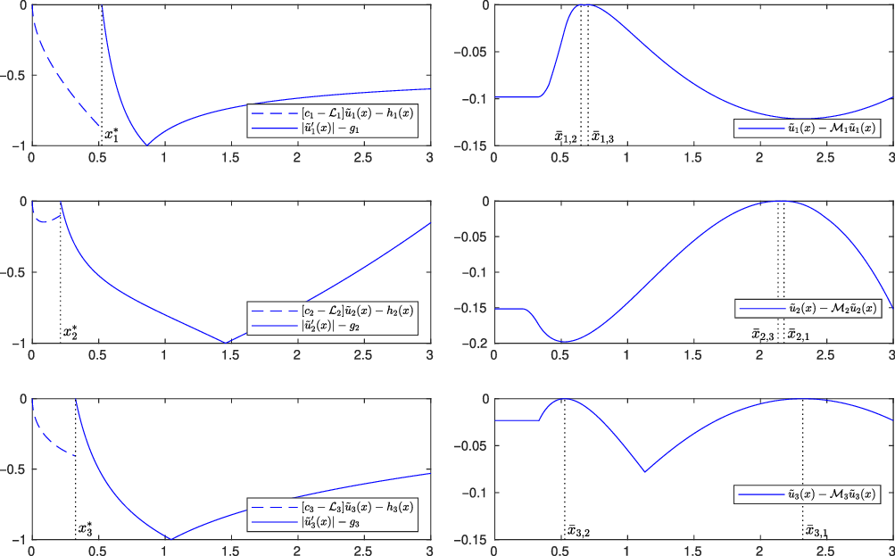
Figure 3. The figures in the left column show the plots of
 $[c_{\ell}-\mathcal{L}_{\ell}]\tilde{u}_{\ell}-h_{\ell}$
and
$[c_{\ell}-\mathcal{L}_{\ell}]\tilde{u}_{\ell}-h_{\ell}$
and
 $\big|\tilde{u}^{\prime}_{\ell}\big|-g_{\ell}$
on
$\big|\tilde{u}^{\prime}_{\ell}\big|-g_{\ell}$
on
 $\big(0,x^{*}_{\ell}\big)$
and
$\big(0,x^{*}_{\ell}\big)$
and
 $\big(x^{*}_{\ell}, l\big)$
, respectively. The figures in the right column show the plots of
$\big(x^{*}_{\ell}, l\big)$
, respectively. The figures in the right column show the plots of
 $\tilde{u}_{\ell}-\mathcal{M}_{\ell}\tilde{u}_{\ell}$
on (0,l).
$\tilde{u}_{\ell}-\mathcal{M}_{\ell}\tilde{u}_{\ell}$
on (0,l).
6. Conclusions and some further work
The main contribution of our paper consists in combining singular and switching controls for the general diffusion model on a bounded domain. Under Assumptions (H1)–(H4), we showed that the existence and uniqueness of the strong solutions to the HJB equations (2.9) and (2.20) are guaranteed on the space
 $\textrm{C}^{0,1}\big(\overline{\mathcal{O}}\big)\cap \textrm{W}^{2,\infty}_{\textrm{loc}}(\mathcal{O})$
. After that, we proved that the value function
$\textrm{C}^{0,1}\big(\overline{\mathcal{O}}\big)\cap \textrm{W}^{2,\infty}_{\textrm{loc}}(\mathcal{O})$
. After that, we proved that the value function
 $V^{\varepsilon}$
for the
$V^{\varepsilon}$
for the
 $\varepsilon$
-PACS control problem seen in Subsection 2.2 satisfies (2.20), showing that for
$\varepsilon$
-PACS control problem seen in Subsection 2.2 satisfies (2.20), showing that for
 $\ell\in\mathbb{I}$
,
$\ell\in\mathbb{I}$
,
 $V^{\varepsilon}_{\ell}\in \textrm{C}^{0,1}\big(\overline{\mathcal{O}}\big)\cap \textrm{W}^{2,\infty}_{\textrm{loc}}(\mathcal{O})$
. Finally, assuming also that the domain set
$V^{\varepsilon}_{\ell}\in \textrm{C}^{0,1}\big(\overline{\mathcal{O}}\big)\cap \textrm{W}^{2,\infty}_{\textrm{loc}}(\mathcal{O})$
. Finally, assuming also that the domain set
 $\mathcal{O}$
is an open convex set and by probabilistic arguments, we verified that the value function V, given in (2.8), is characterized as a limit of
$\mathcal{O}$
is an open convex set and by probabilistic arguments, we verified that the value function V, given in (2.8), is characterized as a limit of
 $V^{\varepsilon}$
as
$V^{\varepsilon}$
as
 $\varepsilon\downarrow0$
, which permitted us to conclude that V satisfies (2.9) and, from here, to see that for
$\varepsilon\downarrow0$
, which permitted us to conclude that V satisfies (2.9) and, from here, to see that for
 $\ell\in\mathbb{I}$
,
$\ell\in\mathbb{I}$
,
 $V_{\ell}\in \textrm{C}^{0,1}\big(\overline{\mathcal{O}}\big)\cap \textrm{W}^{2,\infty}_{\textrm{loc}}(\mathcal{O})$
.
$V_{\ell}\in \textrm{C}^{0,1}\big(\overline{\mathcal{O}}\big)\cap \textrm{W}^{2,\infty}_{\textrm{loc}}(\mathcal{O})$
.
Although the optimal control process for the mixed singular/switching stochastic control problem (2.8) was not given explicitly, and this is still an open problem, we constructed a family of
 $\varepsilon$
-PACS optimal control processes
$\varepsilon$
-PACS optimal control processes
 $\big\{\big(\xi^{\varepsilon_{n},*},\varsigma^{\varepsilon_{n},*}\big)\big\}_{n\geq1}$
(see (4.6)–(4.13)) such that the limit of their value functions
$\big\{\big(\xi^{\varepsilon_{n},*},\varsigma^{\varepsilon_{n},*}\big)\big\}_{n\geq1}$
(see (4.6)–(4.13)) such that the limit of their value functions
 $V^{\varepsilon_{n}}$
(as
$V^{\varepsilon_{n}}$
(as
 $\varepsilon_{n}\rightarrow0$
) agrees with the value function V.
$\varepsilon_{n}\rightarrow0$
) agrees with the value function V.
There are many extensions to be considered and directions for future research. Some of them could be as follows:
-
1. To study the value function V given in (2.8) when the infinitesimal generator of the process
$ X^{\xi,\varsigma}$
, without the influence of the singular control
$\xi$
in
$X^{\xi,\varsigma}$
, within the regime
$\ell$
, is given by where
\begin{align*} \mathcal{L}_{\ell} u_{\ell} &=\textrm{tr}\big[a_{\ell} \textrm{D}^{2}u_{\ell} \big]-\big\langle b _{\ell} ,\textrm{D}^{1}u_{\ell} \big\rangle\\ &\quad+\int_{\mathbb{R}^{d}_{*}}\big[u_{\ell}(x+z)-u_{\ell}(x)-\big\langle \textrm{D}^{1}u_{\ell},z\big\rangle\unicode{x1D7D9}_{\{|z|\in(0,1)\}}\big]s_{\ell}(x,z)\nu(\textrm{d} z), \end{align*}
$\nu$
is a Radon measure on
$\mathbb{R}^{d}_{*}\,:\!=\, \mathbb{R}^{d}\setminus\{0\}$
satisfying
$\int_{\mathbb{R}^{d}_{*}}\big[|z|^{2}\wedge 1\big]\nu(\textrm{d} z)< \infty$
, and
$s_{\ell}\,:\,\overline{\mathcal{O}}\times\mathbb{R}^{d}\longrightarrow[0,1]$
is such that for
\begin{equation*}\int_{\mathbb{R}^{d}_{*}}s_{\ell}(x,z)\unicode{x1D7D9}_{\{x+z\notin\mathcal{O}\}}\nu(\textrm{d} z)<\infty\end{equation*}
$x\in\mathcal{O}$
. In this case, the main difficulty lies in obtaining some a priori estimates of
$\int_{\{|z|\in(0,1)\}}\big[\int_{0}^{1} \big|\textrm{D}^{2}u^{\varepsilon}(\cdot+\ tz)\big|\textrm{d} t\big]|z|^{2}s_{\ell}(\cdot,z)\nu(\textrm{d} z)$
that are independent of
$\varepsilon$
.
-
2. To analyze the problem given in (1.1)–(1.3) on the whole space
$\mathbb{R}^{d}$
. In this direction, a technically involved problem could be studied when the controlled process can switch between m-regimes which are governed by Brownian motions with different drifts. -
3. Additionally, this problem could be extended to verify that the value function V given in (2.8) is a viscosity solution to the HJB equation (2.9) on unbounded sets when the ellipticity condition (2.11) is omitted. Recall that the viscosity solutions for problems of this type were studied in [Reference Azcue and Muler2, Reference Chevalier, Ly Vath and Scotti4, Reference Ly Vath, Pham and Villeneuve15] and [Reference Chevalier, Gaïgi and Ly Vath3] for the cases of
$\mathbb{R}$
and
$\mathbb{R}^ 2$
, respectively.


Appendix A. Proofs of Lemma 3.1 and Proposition 3.1
Recall that Lemma 3.1 and Proposition 3.1 are under Assumptions (H1)–(H4). Let us first show (3.2) and (3.3) of Lemma 3.1, which helps to verify the existence of the classic solution
 $u^{\varepsilon, \delta}$
to the NPDS (3.1). Afterwards, to complete the proof of Proposition 3.1, we shall prove (3.4) of Lemma 3.1. From now on, for simplicity of notation, we replace
$u^{\varepsilon, \delta}$
to the NPDS (3.1). Afterwards, to complete the proof of Proposition 3.1, we shall prove (3.4) of Lemma 3.1. From now on, for simplicity of notation, we replace
 $u^{\varepsilon,\delta}$
by u in the proofs.
$u^{\varepsilon,\delta}$
by u in the proofs.
A.1. Verification of Equations (3.2) and (3.3)
Proof of Lemma 3.1. Equation (3.2). Let
 $(x_{0},\ell_{0})\in\overline{\mathcal{O}}\times\mathbb{I}$
be such that
$(x_{0},\ell_{0})\in\overline{\mathcal{O}}\times\mathbb{I}$
be such that
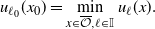 \begin{equation*}u_{\ell_{0}}(x_{0})=\min_{x\in \overline{\mathcal{O}},\ell\in\mathbb{I}}u_{\ell}(x).\end{equation*}
If
 $x_{0}\in\partial\mathcal{O}$
, it follows easily that
$x_{0}\in\partial\mathcal{O}$
, it follows easily that
 $u_{\ell}(x)\geq u_{\ell_{0}}(x_{0})=0$
for all
$u_{\ell}(x)\geq u_{\ell_{0}}(x_{0})=0$
for all
 $(x,\ell)\in\overline{\mathcal{O}}\times\mathbb{I}$
. Suppose that
$(x,\ell)\in\overline{\mathcal{O}}\times\mathbb{I}$
. Suppose that
 $x_{0}\in\mathcal{O}$
. Since
$x_{0}\in\mathcal{O}$
. Since
 $u_{\ell_{0}}=0$
in
$u_{\ell_{0}}=0$
in
 $\partial\mathcal{O}$
, we have that
$\partial\mathcal{O}$
, we have that
 $u_{\ell_{0}}(x_{0})\leq0$
. On the other hand, we know that
$u_{\ell_{0}}(x_{0})\leq0$
. On the other hand, we know that
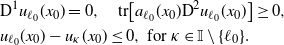 \begin{align} &\textrm{D}^{1} u_{\ell_{0}}(x_{0})=0,\quad \textrm{tr}\big[a_{\ell_{0}}(x_{0})\textrm{D}^{2}u_{\ell_{0}}(x_{0})\big]\geq0,\\ &u_{\ell_{0}}(x_{0})-u_{\kappa}(x_{0})\leq 0,\ \text{for}\ \kappa\in\mathbb{I}\setminus\{\ell_{0}\}. \end{align}
Then, using (H3), (3.1), and (A.1),
 \begin{equation*}0\leq \textrm{tr}\big[a_{\ell_{0}}\textrm{D}^{2}u_{\ell_{0}}\big]= c_{\ell_{0}}u_{\ell_{0}}-h_{\ell_{0}}\leq c_{\ell_{0}}u_{\ell_{0}},\quad \text{at}\ x_{0}.\end{equation*}
Since
 $c_{\ell_{0}}>0$
on
$c_{\ell_{0}}>0$
on
 $\overline{\mathcal{O}}$
, it follows that
$\overline{\mathcal{O}}$
, it follows that
 $u_{\ell_{0}}(x_{0})\geq0$
. Therefore
$u_{\ell_{0}}(x_{0})\geq0$
. Therefore
 $u_{\ell}(x)\geq u_{\ell_{0}}(x_{0})=0$
, for all
$u_{\ell}(x)\geq u_{\ell_{0}}(x_{0})=0$
, for all
 $x\in\overline{\mathcal{O}}$
and
$x\in\overline{\mathcal{O}}$
and
 $\ell\in\mathbb{I}$
.
$\ell\in\mathbb{I}$
.
For each
 $\ell\in\mathbb{I}$
, consider
$\ell\in\mathbb{I}$
, consider
 $\tilde{v}_{\ell}$
as the unique solution to the Dirichlet problem
$\tilde{v}_{\ell}$
as the unique solution to the Dirichlet problem
 $[c_{\ell}-\mathcal{L}_{\ell}] \tilde{v}_{\ell}=h_{\ell}$
in
$[c_{\ell}-\mathcal{L}_{\ell}] \tilde{v}_{\ell}=h_{\ell}$
in
 $\mathcal{O}$
, such that
$\mathcal{O}$
, such that
 $\tilde{v}_{\ell}=0$
on
$\tilde{v}_{\ell}=0$
on
 $\partial\mathcal{O}$
. By Theorem 1.2.10 of [Reference Garroni and Menaldi9], it is well known that
$\partial\mathcal{O}$
. By Theorem 1.2.10 of [Reference Garroni and Menaldi9], it is well known that
 $\tilde{v}_{\ell}\in \textrm{C}^{2,\alpha^{\prime}}\big(\overline{\mathcal{O}}\big)$
and
$\tilde{v}_{\ell}\in \textrm{C}^{2,\alpha^{\prime}}\big(\overline{\mathcal{O}}\big)$
and
 \begin{equation*}||\tilde{v}_{\ell}||_{\textrm{C}^{2,\alpha^{\prime}}\big(\overline{\mathcal{O}}\big)}\leq K_{2} ||h_{\ell}||_{\textrm{C}^{0,\alpha^{\prime}}\big(\overline{\mathcal{O}}\big)}\leq K_{2}\Lambda\,=\!:\, C_{1}, \end{equation*}
where
 $K_{2}=K_{2}(d,\Lambda ,\alpha^{\prime})$
, since (H2)–(H4) hold. Meanwhile, from Equation (3.1), it can be seen that for each
$K_{2}=K_{2}(d,\Lambda ,\alpha^{\prime})$
, since (H2)–(H4) hold. Meanwhile, from Equation (3.1), it can be seen that for each
 $\ell\in\mathbb{I}$
,
$\ell\in\mathbb{I}$
,
 $ [c_{\ell}-\mathcal{L}_{\ell}]u_{\ell}\leq h_{\ell}$
in
$ [c_{\ell}-\mathcal{L}_{\ell}]u_{\ell}\leq h_{\ell}$
in
 $\mathcal{O}$
. Then, taking
$\mathcal{O}$
. Then, taking
 $\eta_{\ell}\,:\!=\, u_{\ell}-\tilde{v}_{\ell}$
, we get, for each
$\eta_{\ell}\,:\!=\, u_{\ell}-\tilde{v}_{\ell}$
, we get, for each
 $\ell\in\mathbb{I}$
,
$\ell\in\mathbb{I}$
,
 \begin{equation} [c_{\ell}-\mathcal{L}_{\ell}]\eta_{\ell}\leq0,\ \text{in}\ \mathcal{O},\quad\text{s.t.}\ \eta_{\ell}=0,\ \text{on}\ \partial\mathcal{O}. \end{equation}
Let
 $x^{*}_{\ell}\in\overline{\mathcal{O}}$
be a maximum point of
$x^{*}_{\ell}\in\overline{\mathcal{O}}$
be a maximum point of
 $\eta_{\ell}$
. If
$\eta_{\ell}$
. If
 $x^{*}_{\ell}\in\partial{\mathcal{O}}$
, trivially we have
$x^{*}_{\ell}\in\partial{\mathcal{O}}$
, trivially we have
 $u_{\ell}-\tilde{v}_{\ell}\leq0$
in
$u_{\ell}-\tilde{v}_{\ell}\leq0$
in
 $\overline{\mathcal{O}}$
. Suppose that
$\overline{\mathcal{O}}$
. Suppose that
 $x^{*}_{\ell}\in \mathcal{O}$
. Note that
$x^{*}_{\ell}\in \mathcal{O}$
. Note that
 $\eta_{\ell}\big(x^{*}_{\ell}\big)\geq0$
and
$\eta_{\ell}\big(x^{*}_{\ell}\big)\geq0$
and
 \begin{equation} \textrm{D}^{1}\eta_{\ell}\big(x^{*}_{\ell}\big)=0,\quad \textrm{tr}\big[a_{\ell}\big(x^{*}_{\ell}\big)\textrm{D}^{2}\eta_{\ell}\big(x^{*}_{\ell}\big)\big]\leq 0. \end{equation}
Then, using (A.2)–(A.3), we have
 $0\geq \textrm{tr}\big[a_{\ell}\textrm{D}^{2}\eta_{\ell}\big]\geq c_{\ell}\eta_{\ell}$
at
$0\geq \textrm{tr}\big[a_{\ell}\textrm{D}^{2}\eta_{\ell}\big]\geq c_{\ell}\eta_{\ell}$
at
 $x^{*}_{\ell}$
. Hence,
$x^{*}_{\ell}$
. Hence,
 $\eta_{\ell}\leq0$
at
$\eta_{\ell}\leq0$
at
 $x^{*}_{\ell}$
, since
$x^{*}_{\ell}$
, since
 $c_{\ell}>0$
on
$c_{\ell}>0$
on
 $\overline{\mathcal{O}}$
. We conclude that
$\overline{\mathcal{O}}$
. We conclude that
 $[u_{\ell}-{\tilde{v}}_{\ell}](x)\leq[u_{\ell}-{\tilde{v}}_{\ell}]\big(x^{*}_{\ell}\big)=0$
for
$[u_{\ell}-{\tilde{v}}_{\ell}](x)\leq[u_{\ell}-{\tilde{v}}_{\ell}]\big(x^{*}_{\ell}\big)=0$
for
 $x\in\overline{\mathcal{O}}$
. Therefore, for each
$x\in\overline{\mathcal{O}}$
. Therefore, for each
 $\ell\in\mathbb{I}$
,
$\ell\in\mathbb{I}$
,
 $0\leq u_{\ell}\leq C_{1}$
on
$0\leq u_{\ell}\leq C_{1}$
on
 $\overline{\mathcal{O}}$
.
$\overline{\mathcal{O}}$
.
Proof of Lemma 3.1. Equation (3.3). For each
 $\ell\in\mathbb{I}$
, consider the auxiliary function
$\ell\in\mathbb{I}$
, consider the auxiliary function
 $w_{\ell}\,:\!=\,\big|\textrm{D}^{1}u_{\ell}\big|^{2}-\lambda A_{\varepsilon,\delta}u_{\ell}$
on
$w_{\ell}\,:\!=\,\big|\textrm{D}^{1}u_{\ell}\big|^{2}-\lambda A_{\varepsilon,\delta}u_{\ell}$
on
 $\overline{\mathcal{O}}$
, where
$\overline{\mathcal{O}}$
, where
 \begin{equation*}A_{\varepsilon,\delta}\,:\!=\,\max_{(x,\ell)\in\overline{\mathcal{O}}\times\mathbb{I}}\big|\textrm{D}^{1}u_{\ell}(x)\big|\end{equation*}
and
 $\lambda\geq1$
is a constant that will be selected later on. Observe that if
$\lambda\geq1$
is a constant that will be selected later on. Observe that if
 $ A_{\varepsilon,\delta}\leq1$
, we obtain a bound for
$ A_{\varepsilon,\delta}\leq1$
, we obtain a bound for
 $ A_{\varepsilon,\delta}$
that is independent of
$ A_{\varepsilon,\delta}$
that is independent of
 $\varepsilon,\delta$
. Hence, we obtain the statement given in the lemma above. We assume henceforth that
$\varepsilon,\delta$
. Hence, we obtain the statement given in the lemma above. We assume henceforth that
 $ A_{\varepsilon,\delta}>1$
. Taking first and second derivatives to
$ A_{\varepsilon,\delta}>1$
. Taking first and second derivatives to
 $w_{\ell}$
, it can be checked that
$w_{\ell}$
, it can be checked that
 \begin{align} -\textrm{tr}\big[a_{\ell}\textrm{D}^{2}w_{\ell}\big]&=-2\sum_{i}\Big\langle a_{\ell}\textrm{D}^{1}\partial_{i}u_{\ell},\textrm{D}^{1}\partial_{i}u_{\ell}\Big\rangle\notag\\ &\quad-2\sum_{i}\textrm{tr} \big[a_{\ell}\textrm{D}^{2}\partial_{i}u_{\ell}\big]\partial_{i}u_{\ell}+\lambda A_{\varepsilon,\delta}\textrm{tr}\big[a_{\ell}\textrm{D}^{2}u_{\ell}\big]. \end{align}
Meanwhile, from (2.3) and (3.1),
 \begin{equation} \lambda A_{\varepsilon,\delta}\textrm{tr}\big[a_{\ell}\textrm{D}^{2} u_{\ell}\big]= \lambda A_{\varepsilon,\delta}\bigg[\widetilde{{D}}_{1}u_{\ell}+\psi_{\varepsilon,\ell}({\cdot})+\displaystyle\sum_{\kappa\in\mathbb{I}\setminus\{\ell\}}\psi_{\delta,\ell,\kappa}({\cdot}) \bigg], \end{equation}
where
 $\psi_{\varepsilon,\ell}({\cdot})$
,
$\psi_{\varepsilon,\ell}({\cdot})$
,
 $\psi_{\delta,\ell,\kappa}({\cdot})$
denote
$\psi_{\delta,\ell,\kappa}({\cdot})$
denote
 $\psi_{\varepsilon}\Big(\big|\textrm{D}^{1}u_{\ell}\big|^{2}-g_{\ell}^{2}\Big)$
,
$\psi_{\varepsilon}\Big(\big|\textrm{D}^{1}u_{\ell}\big|^{2}-g_{\ell}^{2}\Big)$
,
 $\psi_{\delta}\big(u_{\ell}-u_{\kappa} -\vartheta_{\ell,\kappa}\big)$
, respectively, and
$\psi_{\delta}\big(u_{\ell}-u_{\kappa} -\vartheta_{\ell,\kappa}\big)$
, respectively, and
 $\widetilde{D}_{1}u_{\ell}\,:\!=\,\langle b_{\ell},\textrm{D}^{1}u_{\ell}\rangle+c_{\ell}u_{\ell}-h_{\ell}$
. Now, differentiating (3.1), multiplying by
$\widetilde{D}_{1}u_{\ell}\,:\!=\,\langle b_{\ell},\textrm{D}^{1}u_{\ell}\rangle+c_{\ell}u_{\ell}-h_{\ell}$
. Now, differentiating (3.1), multiplying by
 $2\partial_{i}u_{\ell}$
, and taking the summation over all i, we see that
$2\partial_{i}u_{\ell}$
, and taking the summation over all i, we see that
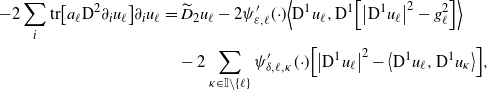 \begin{align} -2\sum_{i}\textrm{tr}\big[a_{\ell}\textrm{D}^{2}\partial_{i} u_{\ell}\big]\partial_{i} u_{\ell} &=\widetilde{D}_{2} u_{\ell} -2\psi^{\prime}_{\varepsilon,\ell}({\cdot})\Big\langle \textrm{D}^{1} u_{\ell},\textrm{D}^{1}\Big[\big|\textrm{D}^{1} u_{\ell}\big|^{2}-g_{\ell}^{2}\Big]\Big\rangle\notag\\ &\quad-2\sum_{\kappa\in\mathbb{I}\setminus\{\ell\}}\psi^{\prime}_{\delta,\ell,\kappa}({\cdot})\Big[\big|\textrm{D}^{1}u_{\ell}\big|^{2}-\big\langle \textrm{D}^{1}u_{\ell},\textrm{D}^{1}u_{\kappa} \big\rangle\Big], \end{align}
where
 \begin{equation} \widetilde{D}_{2}u_{\ell}\,:\!=\, 2\sum_{k}\partial_{k}u_{\ell}\textrm{tr}\big[\big[\partial_{k}a_{\ell}\big]\textrm{D}^{2}u_{\ell}\big] -2\big\langle \textrm{D}^{1}u_{\ell},\textrm{D}^{1}\big[\big\langle b_{\ell},\textrm{D}^{1}u_{\ell}\big\rangle+c_{\ell}u_{\ell}-h_{\ell}\big]\big\rangle. \end{equation}
Then, from (A.4)–(A.6), it can be shown that
 \begin{align*} -\textrm{tr}\big[a_{\ell}\textrm{D}^{2}w_{\ell}\big]&=-2\sum_{i}\big\langle a_{\ell}\textrm{D}^{1}\partial_{i}u_{\ell},\textrm{D}^{1}\partial_{i}u_{\ell}\big\rangle+\widetilde{D}_{2}u_{\ell} +\lambda A_{\varepsilon,\delta} \widetilde{D}_{1}u_{\ell}\notag\\ &\quad-2\psi^{\prime}_{\varepsilon,\ell}({\cdot})\Big\langle \textrm{D}^{1}u_{\ell},\textrm{D}^{1}\Big[\big|\textrm{D}^{1}u_{\ell}\big|^{2}-g_{\ell}^{2}\Big]\Big\rangle+\lambda A_{\varepsilon,\delta}\psi_{\varepsilon,\ell}({\cdot})\notag\\ &\quad-\sum_{\kappa\in\mathbb{I}\setminus\{\ell\}}\Big\{2\psi^{\prime}_{\delta,\ell,\kappa}({\cdot})\Big[\big|\textrm{D}^{1}u_{\ell}\big|^{2}-\big\langle \textrm{D}^{1}u_{\ell},\textrm{D}^{1}u_{\kappa} \big\rangle\Big]-\lambda A_{\varepsilon,\delta}\psi_{\delta,\ell,\kappa}({\cdot})\Big\},\ \end{align*}
on
 $\mathcal{O}$
. Notice that by (H3), (H4), and (3.2),
$\mathcal{O}$
. Notice that by (H3), (H4), and (3.2),
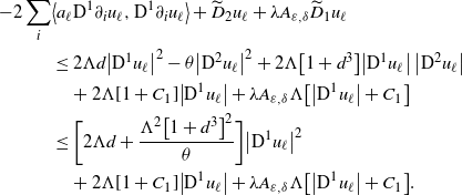 \begin{align} -2\sum_{i}&\big\langle a_{\ell}\textrm{D}^{1}\partial_{i}u_{\ell},\textrm{D}^{1}\partial_{i}u_{\ell}\big\rangle+\widetilde{D}_{2}u_{\ell} +\lambda A_{\varepsilon,\delta} \widetilde{D}_{1}u_{\ell}\notag\\ &\leq2\Lambda d\big|\textrm{D}^{1}u_{\ell}\big|^{2}-\theta\big|\textrm{D}^{2}u_{\ell}\big|^{2}+2\Lambda\big[1+d^{3}\big]\big|\textrm{D}^{1}u_{\ell}\big|\,\big|\textrm{D}^{2}u_{\ell}\big|\notag\\ &\quad+2\Lambda[1+C_{1}]\big|\textrm{D}^{1}u_{\ell}\big|+\lambda A_{\varepsilon,\delta}\Lambda\big[\big|\textrm{D}^{1}u_{\ell}\big|+C_{1}\big]\notag\\ &\leq\bigg[2\Lambda d+\frac{\Lambda^{2}\big[1+d^{3}\big]^{2}}{\theta}\bigg]\big|\textrm{D}^{1}u_{\ell}\big|^{2}\notag\\ &\quad+2\Lambda[1+C_{1}]\big|\textrm{D}^{1}u_{\ell}\big|+\lambda A_{\varepsilon,\delta}\Lambda\big[\big|\textrm{D}^{1}u_{\ell}\big|+C_{1}\big]. \end{align}
Then, by (A.8) and using the convexity property of
 $\psi_{\cdot}$
, i.e.
$\psi_{\cdot}$
, i.e.
 $\psi_{\cdot}(r)\leq \psi^{\prime}_{\cdot}(r)r$
for all
$\psi_{\cdot}(r)\leq \psi^{\prime}_{\cdot}(r)r$
for all
 $r\in\mathbb{R}$
, we see that
$r\in\mathbb{R}$
, we see that
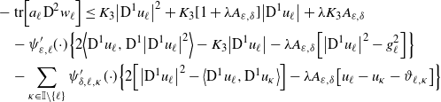 \begin{align} &-\textrm{tr}\Big[a_{\ell}\textrm{D}^{2}w_{\ell}\Big]\leq K_{3}\big|\textrm{D}^{1}u_{\ell}\big|^{2}+K_{3} [1+ \lambda A_{\varepsilon,\delta}]\big|\textrm{D}^{1}u_{\ell}\big|+\lambda K_{3} A_{\varepsilon,\delta}\notag\\ &\quad-\psi^{\prime}_{\varepsilon,\ell}({\cdot})\Big\{2\Big\langle \textrm{D}^{1}u_{\ell},\textrm{D}^{1}\big|\textrm{D}^{1}u_{\ell}\big|^{2}\Big\rangle-K_{3}\big|\textrm{D}^{1}u_{\ell}\big|-\lambda A_{\varepsilon,\delta} \Big[\big|\textrm{D}^{1}u_{\ell}\big|^{2}- g_{\ell}^{2}\Big]\Big\}\notag\\ &\quad-\sum_{\kappa\in\mathbb{I}\setminus\{\ell\}}\psi^{\prime}_{\delta,\ell,\kappa}({\cdot})\Big\{2\Big[\big|\textrm{D}^{1}u_{\ell}\big|^{2}-\big\langle \textrm{D}^{1}u_{\ell},\textrm{D}^{1}u_{\kappa} \big\rangle\Big]-\lambda A_{\varepsilon,\delta}\big[u_{\ell}-u_{\kappa} -\vartheta_{\ell,\kappa}\big]\Big\} \end{align}
on
 $\mathcal{O}$
, for some
$\mathcal{O}$
, for some
 $K_{3}=K_{3}(d,\Lambda ,\alpha^{\prime})$
. Let
$K_{3}=K_{3}(d,\Lambda ,\alpha^{\prime})$
. Let
 $(x_{\lambda},\ell_{\lambda})\in\overline{\mathcal{O}}\times\mathbb{I}$
(depending on
$(x_{\lambda},\ell_{\lambda})\in\overline{\mathcal{O}}\times\mathbb{I}$
(depending on
 $\lambda$
) be such that
$\lambda$
) be such that
 $w_{\ell_{\lambda}}(x_{\lambda})=\max_{(x,\ell)\in\overline{\mathcal{O}}\times\mathbb{I}}w_{\ell}(x)$
. From here, (3.2), and by definition of
$w_{\ell_{\lambda}}(x_{\lambda})=\max_{(x,\ell)\in\overline{\mathcal{O}}\times\mathbb{I}}w_{\ell}(x)$
. From here, (3.2), and by definition of
 $w_{\ell}$
, we see that
$w_{\ell}$
, we see that
 \begin{align} \big|\textrm{D}^{1}u_{\ell}(x)\big|^{2} &\leq\big|\textrm{D}^{1}u_{\ell_{\lambda}}(x_{\lambda})\big|^{2}+\lambda A_{\varepsilon,\delta}C_{1},\quad {\text{for}\ (x,\ell)\in \overline{\mathcal{O}}\times\mathbb{I}.} \end{align}
So it suffices to bound
 $\big|\textrm{D}^{1}u_{\ell_{\lambda}}(x_{\lambda})\big|^{2}$
by a positive constant
$\big|\textrm{D}^{1}u_{\ell_{\lambda}}(x_{\lambda})\big|^{2}$
by a positive constant
 $C=C(d,\Lambda,\alpha^{\prime})$
. If
$C=C(d,\Lambda,\alpha^{\prime})$
. If
 $x_{\lambda}\in\partial \mathcal{O}$
, by (3.2), it can be verified that
$x_{\lambda}\in\partial \mathcal{O}$
, by (3.2), it can be verified that
 $\big|\textrm{D}^{1}u_{\ell_{\lambda}}\big|\leq d^{\frac{1}{2}}C_{1}$
on
$\big|\textrm{D}^{1}u_{\ell_{\lambda}}\big|\leq d^{\frac{1}{2}}C_{1}$
on
 $\partial{\mathcal{O}}$
. Then, from (A.10),
$\partial{\mathcal{O}}$
. Then, from (A.10),
 \begin{equation} \big|\textrm{D}^{1}u_{\ell}(x)\big|^{2}\leq C_{1}\big[dC_{1}+\lambda A_{\varepsilon,\delta}\big] ,\quad {\text{for}\ (x,\ell)\in\overline{\mathcal{O}}\times\mathbb{I}.} \end{equation}
On the other hand, observe that for each
 $\varrho>0$
, there exists
$\varrho>0$
, there exists
 $x_{\varrho}\in\overline{\mathcal{O}}$
such that
$x_{\varrho}\in\overline{\mathcal{O}}$
such that
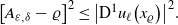 \begin{equation} \big[ A_{\varepsilon,\delta}-\varrho\big]^{2}\leq\big|\textrm{D}^{1} u_{\ell}\big(x_{\varrho}\big)\big|^{2}. \end{equation}
Using (A.11) in (A.12) and letting
 $\varrho\rightarrow0$
, we have
$\varrho\rightarrow0$
, we have
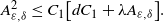 \begin{equation} A_{\varepsilon,\delta}^{2}\leq C_{1}\big[dC_{1}+\lambda A_{\varepsilon,\delta}\big] . \end{equation}
Multiplying by
 $1/A_{\varepsilon,\delta}$
in (A.13), and since
$1/A_{\varepsilon,\delta}$
in (A.13), and since
 $A_{\varepsilon,\delta}>1$
, we get
$A_{\varepsilon,\delta}>1$
, we get
 \begin{equation} \big|\textrm{D}^{1}u_{\ell}(x)\big|\leq A_{\varepsilon,\delta}\leq dC_{1}^{2}+\lambda C_{1},\quad \text{for}\ (x,\ell)\in\overline{\mathcal{O}}\times\mathbb{I}. \end{equation}
In this case, considering
 $\lambda>1$
fixed and
$\lambda>1$
fixed and
 $C_{2}\,:\!=\, C_{1}[dC_{1}+\lambda]$
, we obtain the result that is proposed in the lemma. Let
$C_{2}\,:\!=\, C_{1}[dC_{1}+\lambda]$
, we obtain the result that is proposed in the lemma. Let
 $x_{\lambda}$
be in
$x_{\lambda}$
be in
 $\mathcal{O}$
. It is known that
$\mathcal{O}$
. It is known that
 $\partial_{i}\big|\textrm{D}^{1}u_{\ell_{\lambda}}\big|^{2}-\lambda A_{\varepsilon,\delta}\partial_{i}u_{\ell_{\lambda}}=0$
at
$\partial_{i}\big|\textrm{D}^{1}u_{\ell_{\lambda}}\big|^{2}-\lambda A_{\varepsilon,\delta}\partial_{i}u_{\ell_{\lambda}}=0$
at
 $x_{\lambda}$
. Then,
$x_{\lambda}$
. Then,
 \begin{equation} 2\Big\langle \textrm{D}^{1}u_{\ell_{\lambda}},\textrm{D}^{1}\big|\textrm{D}^{1}u_{\ell_{\lambda}}\big|^{2}\Big\rangle=2\lambda A_{\varepsilon,\delta}\big|\textrm{D}^{1}u_{\ell_{\lambda}}\big|^{2},\ \text{at}\ x_{\lambda}. \end{equation}
Also, since
 $\vartheta_{\ell_{\lambda},\kappa}\geq0$
and
$\vartheta_{\ell_{\lambda},\kappa}\geq0$
and
 $w_{\ell_{\lambda}}(x_{\lambda})-w_{\kappa}(x_{\lambda} )\geq0$
for each
$w_{\ell_{\lambda}}(x_{\lambda})-w_{\kappa}(x_{\lambda} )\geq0$
for each
 $\kappa\in\mathbb{I}$
, and
$\kappa\in\mathbb{I}$
, and
 \begin{equation*}|y_{1}|^{2}-|y_{2}|^{2}=2\big[|y_{1}|^{2}-\langle y_{1},y_{2}\rangle\big]-|y_{1}-y_{2}|^{2}\leq2\big[|y_{1}|^{2}-\langle y_{1},y_{2}\rangle\big]\end{equation*}
for
 $y_{1},y_{2}\in\mathbb{R}^{d},$
we have
$y_{1},y_{2}\in\mathbb{R}^{d},$
we have
 \begin{equation} 2\Big[\big|\textrm{D}^{1}u_{\ell_{\lambda}}\big|^{2}-\big\langle \textrm{D}^{1}u_{\ell_{\lambda}},\textrm{D}^{1}u_{\kappa} \big\rangle\Big]-\lambda A_{\varepsilon,\delta}\big[u_{\ell_{\lambda}}-u_{\kappa} -\vartheta_{\ell_{\lambda},\kappa}\big]\geq0,\ \text{at}\ x_{\lambda}. \end{equation}
By (A.9), (A.15), and (A.16), and since
 $\textrm{tr}\big[a_{\ell_{\lambda}}(x_{\lambda})\textrm{D}^{2}w_{\ell_{\lambda}}(x_{\lambda})\big]\leq0$
, we have
$\textrm{tr}\big[a_{\ell_{\lambda}}(x_{\lambda})\textrm{D}^{2}w_{\ell_{\lambda}}(x_{\lambda})\big]\leq0$
, we have
 \begin{align} 0\leq-\textrm{tr}\big[a_{\ell_{\lambda}}\textrm{D}^{2}w_{\ell_{\lambda}}\big]&\leq K_{3}\big|\textrm{D}^{1}u_{\ell_{\lambda}}\big|^{2}+K_{3} \big[1+ \lambda A_{\varepsilon,\delta}\big]\big|\textrm{D}^{1}u_{\ell_{\lambda}}\big|+\lambda K_{3} A_{\varepsilon,\delta}\notag\\ &\quad-\psi^{\prime}_{\varepsilon,\ell_{\lambda}}({\cdot})\Big[\lambda A_{\varepsilon,\delta}\big|\textrm{D}^{1}u_{\ell_{\lambda}}\big|^{2}-K_{3}\big|\textrm{D}^{1}u_{\ell_{\lambda}}\big|+\lambda A_{\varepsilon,\delta} g_{\ell_{\lambda}}^{2}\Big] \end{align}
at
 $x_{\lambda}$
. On the other hand, notice that either
$x_{\lambda}$
. On the other hand, notice that either
 $\psi^{\prime}_{\varepsilon,\ell_{\lambda}}({\cdot})<\frac{1}{\varepsilon}$
or
$\psi^{\prime}_{\varepsilon,\ell_{\lambda}}({\cdot})<\frac{1}{\varepsilon}$
or
 $\psi^{\prime}_{\varepsilon,\ell_{\lambda}}({\cdot})=\frac{1}{\varepsilon}$
at
$\psi^{\prime}_{\varepsilon,\ell_{\lambda}}({\cdot})=\frac{1}{\varepsilon}$
at
 $x_{\lambda}$
. If
$x_{\lambda}$
. If
 $\psi^{\prime}_{\varepsilon,\ell_{\lambda}}({\cdot})<\frac{1}{\varepsilon}$
at
$\psi^{\prime}_{\varepsilon,\ell_{\lambda}}({\cdot})<\frac{1}{\varepsilon}$
at
 $x_{\lambda}$
, then by the definition of
$x_{\lambda}$
, then by the definition of
 $\psi_{\varepsilon}$
, given in (2.16), it follows that
$\psi_{\varepsilon}$
, given in (2.16), it follows that
 $\big|\textrm{D}^{1}u_{\ell_{\lambda}}(x_{\lambda})\big|^{2}-g_{\ell_{\lambda}}(x_{\lambda})^{2}\leq 2 \varepsilon $
. This implies that
$\big|\textrm{D}^{1}u_{\ell_{\lambda}}(x_{\lambda})\big|^{2}-g_{\ell_{\lambda}}(x_{\lambda})^{2}\leq 2 \varepsilon $
. This implies that
 $\big|\textrm{D}^{1}u_{\ell_{\lambda}}(x_{\lambda})\big|^{2}\leq \Lambda^{2}+2$
. Then, by (A.10) and arguing as in (A.14), we obtain
$\big|\textrm{D}^{1}u_{\ell_{\lambda}}(x_{\lambda})\big|^{2}\leq \Lambda^{2}+2$
. Then, by (A.10) and arguing as in (A.14), we obtain
 $ \big|\textrm{D}^{1}u_{\ell}(x)\big|\leq A_{\varepsilon,\delta}\leq 2+\Lambda^{2}+\lambda C_{1}$
for each
$ \big|\textrm{D}^{1}u_{\ell}(x)\big|\leq A_{\varepsilon,\delta}\leq 2+\Lambda^{2}+\lambda C_{1}$
for each
 $(x,\ell)\in\overline{\mathcal{O}}\times\mathbb{I}$
. For
$(x,\ell)\in\overline{\mathcal{O}}\times\mathbb{I}$
. For
 $\lambda>1$
fixed, this yields the result given in the lemma. Now, assume that
$\lambda>1$
fixed, this yields the result given in the lemma. Now, assume that
 $\psi^{\prime}_{\varepsilon,\ell_{\lambda}}({\cdot})=\frac{1}{\varepsilon}$
. Then, taking
$\psi^{\prime}_{\varepsilon,\ell_{\lambda}}({\cdot})=\frac{1}{\varepsilon}$
. Then, taking
 $\lambda>\max\{1,K_{3}\}$
fixed, using (A.17), and proceeding similarly as for (A.14), we get
$\lambda>\max\{1,K_{3}\}$
fixed, using (A.17), and proceeding similarly as for (A.14), we get
 $0\leq [K_{3}-\lambda]\big|\textrm{D}^{1}u_{\ell_{\lambda}}\big|^{2}+K_{3}[2+\lambda]\big|\textrm{D}^{1}u_{\ell_{\lambda}}\big|+\lambda K_{3}\ \text{at}\ x_{\lambda}$
. From here, we obtain that
$0\leq [K_{3}-\lambda]\big|\textrm{D}^{1}u_{\ell_{\lambda}}\big|^{2}+K_{3}[2+\lambda]\big|\textrm{D}^{1}u_{\ell_{\lambda}}\big|+\lambda K_{3}\ \text{at}\ x_{\lambda}$
. From here, we obtain that
 $\big|\textrm{D}^{1}u_{\ell_{\lambda}}(x_{\lambda})\big|<K_{4}$
for some
$\big|\textrm{D}^{1}u_{\ell_{\lambda}}(x_{\lambda})\big|<K_{4}$
for some
 $K_{4}=K_{4}(d,\Lambda ,\alpha^{\prime})$
. Using (A.10) and by arguments similar to (A.13), we conclude that there exists
$K_{4}=K_{4}(d,\Lambda ,\alpha^{\prime})$
. Using (A.10) and by arguments similar to (A.13), we conclude that there exists
 $C_{2}=C_{2}(d,\Lambda ,\alpha^{\prime})$
such that
$C_{2}=C_{2}(d,\Lambda ,\alpha^{\prime})$
such that
 $\big|\textrm{D}^{1}u_{\ell}\big|\leq A_{\varepsilon,\delta}\leq C_{2}$
on
$\big|\textrm{D}^{1}u_{\ell}\big|\leq A_{\varepsilon,\delta}\leq C_{2}$
on
 $\overline{\mathcal{O}}$
.
$\overline{\mathcal{O}}$
.
A.2. Existence and uniqueness of the solution to the NPDS
Let
 $\mathcal{C}^{k}$
,
$\mathcal{C}^{k}$
,
 $\mathcal{C}^{k,\alpha^{\prime}}$
be the sets given by
$\mathcal{C}^{k,\alpha^{\prime}}$
be the sets given by
 $(\textrm{C}^{k}(\overline{\mathcal{O}}))^{m}$
,
$(\textrm{C}^{k}(\overline{\mathcal{O}}))^{m}$
,
 $(\textrm{C}^{k,\alpha^{\prime}}(\overline{\mathcal{O}}))^{m}$
, respectively, with
$(\textrm{C}^{k,\alpha^{\prime}}(\overline{\mathcal{O}}))^{m}$
, respectively, with
 $k\in\mathbb{N}$
and
$k\in\mathbb{N}$
and
 $\alpha^{\prime}\in(0,1)$
. Defining
$\alpha^{\prime}\in(0,1)$
. Defining
for each ![]() , the reader can verify that
, the reader can verify that
 $||\cdot||_{\mathcal{C}^{k}}$
is a norm on
$||\cdot||_{\mathcal{C}^{k}}$
is a norm on
 $\mathcal{C}^{k}$
and
$\mathcal{C}^{k}$
and
 $(\mathcal{C}^{k},||\cdot||_{\mathcal{C}^{k}})$
is a Banach space.
$(\mathcal{C}^{k},||\cdot||_{\mathcal{C}^{k}})$
is a Banach space.
Notice that for each ![]() fixed, there exists a unique solution
fixed, there exists a unique solution ![]() to the NPDS
to the NPDS
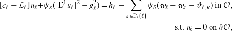
(see [Reference Gilbarg and Trudinger10, Theorem 15.10, p. 380]). Additionally, from [Reference Adams and Fournier1, Theorem 4.12, p. 85] and [Reference Garroni and Menaldi9, Theorem 1.2.19], it follows that

for some
 $K_{5}=K_{5}(d,\Lambda,\alpha^{\prime})$
, where
$K_{5}=K_{5}(d,\Lambda,\alpha^{\prime})$
, where
 $p^{\prime}\in(d,\infty)$
is such that
$p^{\prime}\in(d,\infty)$
is such that
 $\alpha^{\prime}=1-d/p^{\prime}$
. Observe that for each
$\alpha^{\prime}=1-d/p^{\prime}$
. Observe that for each ![]() , we get
, we get ![]() , with
, with
 $\ell\in\mathbb{I}$
. Then, arguing in the same way as in the proof of (3.2), it follows that for each
$\ell\in\mathbb{I}$
. Then, arguing in the same way as in the proof of (3.2), it follows that for each ![]() ,
,
with
 $C_{1}$
as in (3.2). Meanwhile, taking
$C_{1}$
as in (3.2). Meanwhile, taking ![]() , with
, with
and following steps similar to those seen in the proof of (3.3), it can be verified that for each ![]() ,
,
for some constant
 $K_{6}=K_{6}(\Lambda,d,\theta,m,\lambda,1/\delta)$
. We proceed to give the proof of Proposition 3.1.
$K_{6}=K_{6}(\Lambda,d,\theta,m,\lambda,1/\delta)$
. We proceed to give the proof of Proposition 3.1.
Proof of Proposition 3.1. Existence. Define the mapping
 \begin{equation*}T:(\mathcal{C}^{1},||\cdot||_{\mathcal{C}^{1}})\longrightarrow(\mathcal{C}^{1},||\cdot||_{\mathcal{C}^{1}})\end{equation*}
by ![]() for each
for each ![]() , where
, where ![]() is the unique solution to the NDPS (A.18). To use Schaefer’s fixed point theorem (see e.g. [Reference Evans8, Theorem 4, p. 539]), we only need to verify the following: (i) the mapping T is continuous and compact; (ii) the set
is the unique solution to the NDPS (A.18). To use Schaefer’s fixed point theorem (see e.g. [Reference Evans8, Theorem 4, p. 539]), we only need to verify the following: (i) the mapping T is continuous and compact; (ii) the set ![]() is bounded uniformly, i.e.
is bounded uniformly, i.e. ![]() , for each
, for each ![]() , where C is some positive constant that is independent of
, where C is some positive constant that is independent of ![]() and
and
 $\varrho$
.
$\varrho$
.
To verify the first item above, notice that, by (A.19)–(A.21) and by the Arzelà–Ascoli compactness criterion (see [Reference Evans8, Section C.8, p. 718]), T maps bounded sets in
 $\mathcal{C}^{1}$
into bounded sets in itself that are precompact in
$\mathcal{C}^{1}$
into bounded sets in itself that are precompact in
 $\mathcal{C}^{1}$
. With this remark and by the uniqueness of the solution to the NPDS (A.18), the reader can verify that T is a continuous and compact mapping from
$\mathcal{C}^{1}$
. With this remark and by the uniqueness of the solution to the NPDS (A.18), the reader can verify that T is a continuous and compact mapping from
 $\mathcal{C}^{1}$
into itself. Let us prove the second item above. Consider now
$\mathcal{C}^{1}$
into itself. Let us prove the second item above. Consider now ![]() . Observe that if
. Observe that if
 $\varrho=0$
, it follows immediately that
$\varrho=0$
, it follows immediately that ![]() , where
, where
 $\overline{0}$
is the null function. Assume that
$\overline{0}$
is the null function. Assume that ![]() is such that
is such that ![]() for some
for some
 $\varrho\in(0,1]$
, or, in other words,
$\varrho\in(0,1]$
, or, in other words, ![]() and
and
where
By Theorems 6.14 and 9.19 of [Reference Gilbarg and Trudinger10], we have that ![]() , since (H2)–(H4) hold and
, since (H2)–(H4) hold and
 $f_{\ell}\in\textrm{C}^{1,\alpha^{\prime}}(\overline{\mathcal{O}})$
. Then,
$f_{\ell}\in\textrm{C}^{1,\alpha^{\prime}}(\overline{\mathcal{O}})$
. Then,
 $\mathcal{A}\subset\mathcal{C}^{3,\alpha^{\prime}}$
. Observe that
$\mathcal{A}\subset\mathcal{C}^{3,\alpha^{\prime}}$
. Observe that ![]() on
on
 $\overline{\mathcal{O}}$
, because of
$\overline{\mathcal{O}}$
, because of ![]() . Taking
. Taking ![]() , with
, with ![]() , using (A.22) and applying the same arguments seen in the proof of (3.3), one can check that for each
, using (A.22) and applying the same arguments seen in the proof of (3.3), one can check that for each ![]() , we have
, we have
where
 $ C_{2}$
is a positive constant as in Lemma 3.1. Notice that
$ C_{2}$
is a positive constant as in Lemma 3.1. Notice that
 $C_{1}$
and
$C_{1}$
and
 $C_{2}$
are independent of
$C_{2}$
are independent of ![]() and
and
 $\varrho$
. It follows that
$\varrho$
. It follows that
 $\mathcal{A}$
is bounded uniformly. From that, we see that the items above, (i) and (ii), are true, and by Schaefer’s fixed point theorem, there exists a fixed point
$\mathcal{A}$
is bounded uniformly. From that, we see that the items above, (i) and (ii), are true, and by Schaefer’s fixed point theorem, there exists a fixed point
 $u=(u_{1},\dots,u_{m})\in{\mathcal{C}^{1}}$
to the problem
$u=(u_{1},\dots,u_{m})\in{\mathcal{C}^{1}}$
to the problem
 $T[u]=u$
which satisfies the NPDS (3.1). In addition, we have
$T[u]=u$
which satisfies the NPDS (3.1). In addition, we have
 $u=T[u]\in\mathcal{C}^{2,\alpha^{\prime}}$
, and by arguments similar to those seen previously, it can be shown that u is nonnegative and belongs to
$u=T[u]\in\mathcal{C}^{2,\alpha^{\prime}}$
, and by arguments similar to those seen previously, it can be shown that u is nonnegative and belongs to
 $\mathcal{C}^{3,\alpha^{\prime}}(\overline{\mathcal{O}})$
. Again, repeating the same arguments seen above, we can conclude that
$\mathcal{C}^{3,\alpha^{\prime}}(\overline{\mathcal{O}})$
. Again, repeating the same arguments seen above, we can conclude that
 $u\in\mathcal{C}^{4,\alpha^{\prime}}(\overline{\mathcal{O}})$
.
$u\in\mathcal{C}^{4,\alpha^{\prime}}(\overline{\mathcal{O}})$
.
Proof of Proposition 3.1. Uniqueness. The uniqueness of the solution u to the NPDS (3.1) is obtained by contradiction. Assume that there are two solutions
 $u,v\in\mathcal{C}^{4,\alpha^{\prime}}$
to the NPDS (3.1). Let
$u,v\in\mathcal{C}^{4,\alpha^{\prime}}$
to the NPDS (3.1). Let
 $\nu=(\nu_{1},\dots,\nu_{m})\in\mathcal{C}^{4,\alpha^{\prime}}$
be such that
$\nu=(\nu_{1},\dots,\nu_{m})\in\mathcal{C}^{4,\alpha^{\prime}}$
be such that
 $\nu_{\ell}\,:\!=\, u_{\ell}-v_{\ell}$
for
$\nu_{\ell}\,:\!=\, u_{\ell}-v_{\ell}$
for
 $\ell\in\mathbb{I}$
. Let
$\ell\in\mathbb{I}$
. Let
 $(x_{\circ},\ell_{\circ}) \in \overline{\mathcal{O}}\times\mathbb{I}$
be such that
$(x_{\circ},\ell_{\circ}) \in \overline{\mathcal{O}}\times\mathbb{I}$
be such that
 $\nu_{\ell_{\circ}}(x_{\circ})=\max_{(x,\ell)\in\overline{\mathcal{O}}\times\mathbb{I}}\nu_{\ell}(x)$
. If
$\nu_{\ell_{\circ}}(x_{\circ})=\max_{(x,\ell)\in\overline{\mathcal{O}}\times\mathbb{I}}\nu_{\ell}(x)$
. If
 $x_{ \circ}\in\partial{\mathcal{O}}$
, trivially we have
$x_{ \circ}\in\partial{\mathcal{O}}$
, trivially we have
 $u_{\ell}-v_{\ell}\leq0$
in
$u_{\ell}-v_{\ell}\leq0$
in
 $\overline{\mathcal{O}}$
, for
$\overline{\mathcal{O}}$
, for
 $\ell\in\mathbb{I}$
. Suppose that
$\ell\in\mathbb{I}$
. Suppose that
 $x_{\circ}\in \mathcal{O}$
. Then
$x_{\circ}\in \mathcal{O}$
. Then
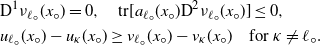 \begin{align}
&\textrm{D}^{1}\nu_{\ell_{\circ}}(x_{\circ})=0,\quad\textrm{tr}[a_{\ell_{\circ}}(x_{\circ})\textrm{D}^{2}\nu_{\ell_{\circ}}(x_{\circ})]\leq 0,\\
&u_{\ell_{\circ}}(x_{\circ})-u_{\kappa}(x_{\circ} )\geq v_{\ell_{\circ}}(x_{\circ})-v_{\kappa}(x_{\circ} )\quad \text{for}\ \kappa\neq\ell_{\circ} .\end{align}
\begin{align}
&\textrm{D}^{1}\nu_{\ell_{\circ}}(x_{\circ})=0,\quad\textrm{tr}[a_{\ell_{\circ}}(x_{\circ})\textrm{D}^{2}\nu_{\ell_{\circ}}(x_{\circ})]\leq 0,\\
&u_{\ell_{\circ}}(x_{\circ})-u_{\kappa}(x_{\circ} )\geq v_{\ell_{\circ}}(x_{\circ})-v_{\kappa}(x_{\circ} )\quad \text{for}\ \kappa\neq\ell_{\circ} .\end{align}
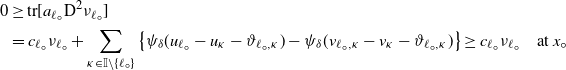 \begin{align} 0&\geq\textrm{tr}[a_{\ell_{\circ}}\textrm{D}^{2}\nu_{\ell_{\circ}}]\notag\\ &=c_{\ell_{\circ}}\nu_{\ell_{\circ}}+\sum_{\kappa\in\mathbb{I}\setminus\{\ell_{\circ}\}}\big\{\psi_{\delta}(u_{\ell_{\circ}}-u_{\kappa} -\vartheta_{\ell_{\circ},\kappa})-\psi_{\delta}(v_{\ell_{\circ},\kappa}-v_{\kappa} -\vartheta_{\ell_{\circ},\kappa})\big\}\geq c_{\ell_{\circ}}\nu_{\ell_{\circ}}\quad \text{at}\ x_{\circ} \end{align}
because of
 \begin{equation*}0\leq\psi_{\delta}(u_{\ell_{\circ}}-u_{\kappa}-\vartheta_{\ell_{\circ},\kappa}) -\psi_{\delta}(v_{\ell_{\circ}}-v_{\kappa}-\vartheta_{\ell_{\circ},\kappa})\end{equation*}
at
 $x_{\circ}$
, for
$x_{\circ}$
, for
 $\kappa\in\mathbb{I}$
. From (A.25) and since
$\kappa\in\mathbb{I}$
. From (A.25) and since
 $c_{\ell_{\circ}}>0$
, we have that
$c_{\ell_{\circ}}>0$
, we have that
 $u_{\ell}(x)-v_{\ell}(x)\leq u_{\ell_{\circ}}(x_{\circ})-v_{\ell_{\circ}}(x_{\circ})\leq0$
for
$u_{\ell}(x)-v_{\ell}(x)\leq u_{\ell_{\circ}}(x_{\circ})-v_{\ell_{\circ}}(x_{\circ})\leq0$
for
 $(x,\ell)\in\overline{\mathcal{O}}\times\mathbb{I}$
. Taking now
$(x,\ell)\in\overline{\mathcal{O}}\times\mathbb{I}$
. Taking now
 $\nu\,:\!=\, v-u$
and proceeding in the same way than before, we obtain immediately that
$\nu\,:\!=\, v-u$
and proceeding in the same way than before, we obtain immediately that
 $v_{{\ell}} -u_{{\ell}}\leq0$
on
$v_{{\ell}} -u_{{\ell}}\leq0$
on
 $\overline{\mathcal{O}}$
for
$\overline{\mathcal{O}}$
for
 $ \ell\in\mathbb{I}$
. Therefore
$ \ell\in\mathbb{I}$
. Therefore
 $u =v$
, and from here we conclude that the NPDS (3.1) has a unique solution u, whose components belong to
$u =v$
, and from here we conclude that the NPDS (3.1) has a unique solution u, whose components belong to
 $\textrm{C}^{4,\alpha^{\prime}}(\overline{\mathcal{O}})$
.
$\textrm{C}^{4,\alpha^{\prime}}(\overline{\mathcal{O}})$
.
A.3. Verification of Equation (3.4)
Let us define the auxiliary function
 $\phi_{\ell}$
by
$\phi_{\ell}$
by
 \begin{equation}\phi_{\ell}\,:\!=\,\omega^{2}\big|\textrm{D}^{2}u_{\ell}\big|^{2}+\lambda A^{1}_{\varepsilon,\delta}\omega \textrm{tr}\big[\alpha_{\ell_{0}}\textrm{D}^{2}u_{\ell}\big]+\mu\big|\textrm{D}^{1}u_{\ell}\big|^{2}\ \text{ on}\ \mathcal{O},\end{equation}
with
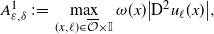 \begin{equation*}A^{1}_{\varepsilon,\delta}\,:\!=\,\max_{(x,\ell)\in\overline{\mathcal{O}}\times\mathbb{I}}\omega(x)\big|\textrm{D}^{2}u_{\ell}(x)\big|,\end{equation*}
 $\lambda\geq\max\{1,2/\theta\}$
,
$\lambda\geq\max\{1,2/\theta\}$
,
 $\mu\geq1$
fixed, and
$\mu\geq1$
fixed, and
 $\alpha_{\ell_{0}}=(\alpha_{\ell_{0}\,ij})_{d\times d}$
such that
$\alpha_{\ell_{0}}=(\alpha_{\ell_{0}\,ij})_{d\times d}$
such that
 $\alpha_{\ell_{0}\,ij}\,:\!=\, a_{\ell_{0}\,ij}(x_{0})$
, where
$\alpha_{\ell_{0}\,ij}\,:\!=\, a_{\ell_{0}\,ij}(x_{0})$
, where
 $(x_{0},\ell_{0})\in\overline{\mathcal{O}}\times\mathbb{I}$
is fixed. Recall that
$(x_{0},\ell_{0})\in\overline{\mathcal{O}}\times\mathbb{I}$
is fixed. Recall that
 $\omega$
is a cut-off function as in Remark 3.1. We shall show that
$\omega$
is a cut-off function as in Remark 3.1. We shall show that
 $\phi_{\ell}$
satisfies (A.25). In particular, (A.25) holds when
$\phi_{\ell}$
satisfies (A.25). In particular, (A.25) holds when
 $\phi_{\ell}$
is evaluated at its maximum
$\phi_{\ell}$
is evaluated at its maximum
 $x_{\mu}\in\mathcal{O}$
, which helps to show that (3.4) is true.
$x_{\mu}\in\mathcal{O}$
, which helps to show that (3.4) is true.
Lemma A.1. Let
 $\phi_{\ell}$
be the auxiliary function given by (A.26). Then there exists a positive constant
$\phi_{\ell}$
be the auxiliary function given by (A.26). Then there exists a positive constant
 $C_{7}=C_{7}(d,\Lambda ,\alpha^{\prime},K_{1})$
such that on
$C_{7}=C_{7}(d,\Lambda ,\alpha^{\prime},K_{1})$
such that on
 $(x,\ell)\in\overline{\mathcal{O}}\times\mathbb{I}$
,
$(x,\ell)\in\overline{\mathcal{O}}\times\mathbb{I}$
,
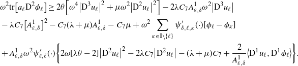 \begin{align} &\omega^{2}\textrm{tr}\big[a_{\ell}\textrm{D}^{2}\phi_{\ell}\big] \geq 2\theta\Big[\omega^{4}\big|\textrm{D}^{3}u_{\ell}\big|^{2}+\mu\omega^{2}\big|\textrm{D}^{2}u_{\ell}\big|^{2}\Big]-2\lambda C_{7}A^{1}_{\varepsilon,\delta}\omega^{2}\big|\textrm{D}^{3}u_{\ell}\big|\notag\\ &-\lambda C_{7}\big[A^{1}_{\varepsilon,\delta}\big]^{2}-C_{7}(\lambda+\mu)A^{1}_{\varepsilon,\delta}-C_{7}\mu+\omega^{2}\sum_{\kappa\in\mathbb{I}\setminus\{\ell\}}\psi^{\prime}_{\delta,\ell,\kappa}({\cdot})[\phi_{\ell}-\phi_{\kappa} ]\notag\\ &+A^{1}_{\varepsilon,\delta}\omega^{2}\psi^{\prime}_{\varepsilon,\ell}({\cdot})\bigg\{2\omega[\lambda\theta-2]\big|\textrm{D}^{2}u_{\ell}\big|^{2}-2\lambda C_{7}\big|\textrm{D}^{2}u_{\ell}\big|-(\lambda+\mu)C_{7}+\frac{2}{A^{1}_{\varepsilon,\delta}}\big\langle \textrm{D}^{1}u_{\ell},\textrm{D}^{1}\phi_{\ell}\big\rangle\bigg\}. \end{align}
Before providing the verification of the lemma above, let us first prove (3.4).
Proof of Lemma 3.1. Equation (3.4). Let
 $\phi_{\ell}$
be as in (A.26), where
$\phi_{\ell}$
be as in (A.26), where
 $\lambda\geq\max\{1,2/\theta\}$
is fixed and
$\lambda\geq\max\{1,2/\theta\}$
is fixed and
 $\mu\geq1$
will be determined later on, and
$\mu\geq1$
will be determined later on, and
 $(x_{0}, \ell_{0})\in\overline{\mathcal{O}}\times\mathbb{I}$
satisfies
$(x_{0}, \ell_{0})\in\overline{\mathcal{O}}\times\mathbb{I}$
satisfies
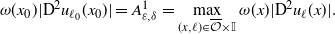 \begin{equation} \omega(x_{0})|\textrm{D}^{2}u_{\ell_{0}}(x_{0})|=A^{1}_{\varepsilon,\delta}=\max_{(x,\ell)\in\overline{\mathcal{O}}\times\mathbb{I}}\omega(x)|\textrm{D}^{2}u_{\ell}(x)|. \end{equation}
Notice that if
 $x_{0}\in\overline{\mathcal{O}}\setminus B_{\beta^{\prime} r}$
, by Remark 3.1 and (A.26), we obtain
$x_{0}\in\overline{\mathcal{O}}\setminus B_{\beta^{\prime} r}$
, by Remark 3.1 and (A.26), we obtain
 $\partial_{ij}u_{\ell}(x)\equiv0$
, for each
$\partial_{ij}u_{\ell}(x)\equiv0$
, for each
 $(x,\ell)\times\overline{\mathcal{O}}\times\mathbb{I}.$
From here, (3.4) is trivially true. So assume that
$(x,\ell)\times\overline{\mathcal{O}}\times\mathbb{I}.$
From here, (3.4) is trivially true. So assume that
 $x_{0}$
is in
$x_{0}$
is in
 $B_{\beta^{\prime}r}$
. Without loss of generality we also assume that
$B_{\beta^{\prime}r}$
. Without loss of generality we also assume that
 $A^{1}_{\varepsilon,\delta}>1$
, since if
$A^{1}_{\varepsilon,\delta}>1$
, since if
 $A^{1}_{\varepsilon,\delta}\leq1$
, we get that
$A^{1}_{\varepsilon,\delta}\leq1$
, we get that
 $\omega(x) \big|\textrm{D}^{2}u_{\ell}(x)\big|\leq A^{1}_{\varepsilon,\delta}\leq1$
for
$\omega(x) \big|\textrm{D}^{2}u_{\ell}(x)\big|\leq A^{1}_{\varepsilon,\delta}\leq1$
for
 $(x,\ell)\in\overline{\mathcal{O}}\times\mathbb{I}$
. Taking
$(x,\ell)\in\overline{\mathcal{O}}\times\mathbb{I}$
. Taking
 $C_{3}=1$
, we obtain the result in (3.4). Let
$C_{3}=1$
, we obtain the result in (3.4). Let
 $(x_{\mu},\ell_{\mu})\in\overline{\mathcal{O}}\times\mathbb{I}$
be such that
$(x_{\mu},\ell_{\mu})\in\overline{\mathcal{O}}\times\mathbb{I}$
be such that
 $\phi_{\ell_{\mu}}(x_{\mu})=\max_{(x,\ell)\in\overline{\mathcal{O}}\times\mathbb{I}}\phi_{\ell}(x)$
. If
$\phi_{\ell_{\mu}}(x_{\mu})=\max_{(x,\ell)\in\overline{\mathcal{O}}\times\mathbb{I}}\phi_{\ell}(x)$
. If
 $x_{\mu}\in\overline{\mathcal{O}}\setminus B_{\beta^{\prime}r}$
, from (3.3) and (A.26) it follows that
$x_{\mu}\in\overline{\mathcal{O}}\setminus B_{\beta^{\prime}r}$
, from (3.3) and (A.26) it follows that
 \begin{equation} \omega^{2}\big|\textrm{D}^{2}u_{\ell}\big|^{2}\leq-\lambda A^{1}_{\varepsilon,\delta}\omega \textrm{tr}\big[\alpha_{\ell_{0}}\textrm{D}^{2}u_{\ell}\big]+\mu C_{2}^{2},\ \text{for}\ (x,\ell)\in\overline{\mathcal{O}}\times\mathbb{I}. \end{equation}
Evaluating
 $(x_{0},l_{0})$
in (A.29) and by (2.3), (H3), (2.16), (3.1), and (3.3), it can be verified that
$(x_{0},l_{0})$
in (A.29) and by (2.3), (H3), (2.16), (3.1), and (3.3), it can be verified that
 $\big[A_{\varepsilon,\delta}^{1}\big]^{2}\leq\lambda\Lambda[1+C_{2}] A_{\varepsilon,\delta}^{1}+\mu C_{2}^{2}$
. From here and because
$\big[A_{\varepsilon,\delta}^{1}\big]^{2}\leq\lambda\Lambda[1+C_{2}] A_{\varepsilon,\delta}^{1}+\mu C_{2}^{2}$
. From here and because
 $A^{1}_{\varepsilon,\delta}>1$
, we conclude that
$A^{1}_{\varepsilon,\delta}>1$
, we conclude that
 \begin{equation*}\omega(x)\big|\textrm{D}^{2}u_{\ell}(x)\big|\leq A_{\varepsilon,\delta}^{1}\leq \lambda\Lambda[1+C_{2}]+\mu C_{2}^{2}\,=\!:\,C_{3},\quad \text{for $(x,\ell)\in\overline{\mathcal{O}}\times\mathbb{I}$.}\end{equation*}
From now on, assume that
 $x_{\mu}\in B_{\beta^{\prime}r}$
. Then
$x_{\mu}\in B_{\beta^{\prime}r}$
. Then
 \begin{align} &\textrm{D}^{1}\phi_{\ell_{\mu}}(x_{\mu})=0, \quad \textrm{tr}\big[a_{\ell_{\mu}}(x_{\mu})\textrm{D}^{2}\phi_{\ell_{\mu}}(x_{\mu})\big]\leq0. \end{align}
Noting that
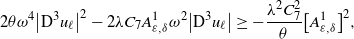 \begin{equation*}2\theta\omega^{4}\big|\textrm{D}^{3}u_{\ell}\big|^{2}-2\lambda C_{7}A^{1}_{\varepsilon,\delta}\omega^{2}\big|\textrm{D}^{3}u_{\ell}\big|\geq-\frac{\lambda^{2}C^{2}_{7}}{\theta}\big[A^{1}_{\varepsilon,\delta}\big]^{2},\end{equation*}
with
 $C_{7}>0$
as in Lemma A.1, and using (A.25) and (A.30), we have that
$C_{7}>0$
as in Lemma A.1, and using (A.25) and (A.30), we have that
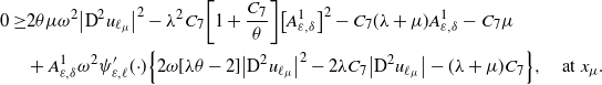 \begin{align*} 0\geq&2\theta\mu\omega^{2}\big|\textrm{D}^{2}u_{\ell_{\mu}}\big|^{2}-\lambda^{2} C_{7}\bigg[1+\frac{C_{7}}{\theta}\bigg]\big[A^{1}_{\varepsilon,\delta}\big]^{2}-C_{7}(\lambda+\mu)A^{1}_{\varepsilon,\delta}-C_{7}\mu\notag\\ &+A^{1}_{\varepsilon,\delta}\omega^{2}\psi^{\prime}_{\varepsilon,\ell}({\cdot})\Big\{2\omega[\lambda\theta-2]\big|\textrm{D}^{2}u_{\ell_{\mu}}\big|^{2}-2\lambda C_{7}\big|\textrm{D}^{2}u_{\ell_{\mu}}\big|-(\lambda+\mu)C_{7}\Big\},\quad \text{at}\ x_{\mu}. \end{align*}
From here, we have that at least one of the following two inequalities is true:
 \begin{align} 2\theta\mu\omega^{2}\big|\textrm{D}^{2}u_{\ell_{\mu}}\big|^{2}-\lambda^{2} C_{7}\bigg[1+\frac{C_{7}}{\theta}\bigg]\big[A^{1}_{\varepsilon,\delta}\big]^{2}-C_{7}(\lambda+\mu)A^{1}_{\varepsilon,\delta}-C_{7}\mu&\leq0,\quad\text{at}\ x_{\mu},\end{align}
 \begin{align} A^{1}_{\varepsilon,\delta}\omega^{2}\psi^{\prime}_{\varepsilon,\ell}({\cdot})\Big\{2\omega[\lambda\theta-2]\big|\textrm{D}^{2}u_{\ell_{\mu}}\big|^{2}-2\lambda C_{7}\big|\textrm{D}^{2}u_{\ell_{\mu}}\big|-(\lambda+\mu)C_{7}\Big\}&\leq0,\quad\text{at}\ x_{\mu}. \end{align}
Suppose that (A.31) holds. Then, evaluating
 $(x_{\mu},\ell_{\mu})$
in (A.26), we get
$(x_{\mu},\ell_{\mu})$
in (A.26), we get
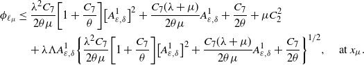 \begin{align} \phi_{\ell_{\mu}} &\leq \frac{\lambda^{2} C_{7}}{2\theta\mu}\bigg[1+\frac{C_{7}}{\theta}\bigg]\big[A^{1}_{\varepsilon,\delta}\big]^{2}+\frac{C_{7}(\lambda+\mu)}{2\theta\mu}A^{1}_{\varepsilon,\delta}+\frac{C_{7}}{2\theta}+\mu C^{2}_{2}\notag\\ &\quad+\lambda\Lambda A^{1}_{\varepsilon,\delta}\bigg\{\frac{\lambda^{2} C_{7}}{2\theta\mu}\bigg[1+\frac{C_{7}}{\theta}\bigg]\big[A^{1}_{\varepsilon,\delta}\big]^{2}+\frac{C_{7}(\lambda+\mu)}{2\theta\mu}A^{1}_{\varepsilon,\delta}+\frac{C_{7}}{2\theta}\bigg\}^{1/2},\quad\text{at}\ x_{\mu}. \end{align}
Meanwhile, evaluating
 $(x_{0},\ell_{0})$
in (A.26) and using (2.3) and (3.1), we get
$(x_{0},\ell_{0})$
in (A.26) and using (2.3) and (3.1), we get
 \begin{align} \phi_{\ell_{0}} \geq\big[A^{1}_{\varepsilon,\delta}\big]^{2}-\lambda \Lambda A^{1}_{\varepsilon,\delta}[C_{2}+1],\quad\text{at}\ x_{0}. \end{align}
Then, taking
 $\mu$
large enough so that
$\mu$
large enough so that
 \begin{equation*}\frac{K_{7}^{(\lambda)}}{\mu}\leq\bigg[\frac{1}{\lambda\Lambda}\bigg[1-\frac{K_{7}^{(\lambda)}}{\mu}\bigg]\bigg]^{2},\end{equation*}
with
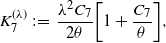 \begin{equation*}K_{7}^{(\lambda)}\,:\!=\,\frac{\lambda^{2}C_{7}}{2\theta}\bigg[1+\frac{C_{7}}{\theta}\bigg],\end{equation*}
using (A.33)–(A.34), and since
 $\phi_{\ell_{0}}(x_{0})\leq\phi_{\ell_{\mu}}(x_{\mu})$
and
$\phi_{\ell_{0}}(x_{0})\leq\phi_{\ell_{\mu}}(x_{\mu})$
and
 $\lambda, A^{1}_{\varepsilon,\delta}>1$
, we have that
$\lambda, A^{1}_{\varepsilon,\delta}>1$
, we have that
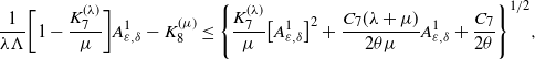 \begin{align*} \frac{1}{\lambda \Lambda}\bigg[1-\frac{K_{7}^{(\lambda)}}{\mu}\bigg]A^{1}_{\varepsilon,\delta}-K_{8}^{(\mu)} \leq\Bigg\{\frac{ K_{7}^{(\lambda)}}{\mu}\big[A^{1}_{\varepsilon,\delta}\big]^{2}+\frac{C_{7}(\lambda+\mu)}{2\theta\mu}A^{1}_{\varepsilon,\delta}+\frac{C_{7}}{2\theta}\Bigg\}^{1/2}, \end{align*}
with
 \begin{equation*}K_{8}^{(\mu)}\,:\!=\,\frac{C_{7}}{2\theta\Lambda}\bigg[\frac{1}{\mu}+1\bigg]+\frac{C_{7}}{2\theta}+\mu C_{2}.\end{equation*}
Then,
 \begin{equation*} \Bigg\{\frac{1}{\lambda^{2} \Lambda^{2}}\Bigg[1-\frac{K_{7}^{(\lambda)}}{\mu}\Bigg]^{2}- \frac{ K_{7}^{(\lambda)}}{\mu}\Bigg\}\big[A^{1}_{\varepsilon,\delta}\big]^{2} \leq\Bigg\{\frac{2K_{8}^{(\mu)}}{\lambda \Lambda}\Bigg[1-\frac{K_{7}^{(\lambda)}}{\mu}\Bigg]+\frac{C_{7}(\lambda+\mu)}{2\theta\mu}\Bigg\}A^{1}_{\varepsilon,\delta}+\frac{C_{7}}{2\theta}. \end{equation*}
From here, we conclude there exists a constant
 $C_{3}=C_{3}(d,\Lambda,\alpha^{\prime},K_{3})$
such that
$C_{3}=C_{3}(d,\Lambda,\alpha^{\prime},K_{3})$
such that
 \begin{equation*} \omega(x)\big|\textrm{D}^{2}u_{\ell}(x)\big|\leq A^{1}_{\varepsilon,\delta}\leq C_{3}\quad \text{for}\ (x,\ell)\in \overline{\mathcal{O}}\times\mathbb{I}. \end{equation*}
Now, assume that (A.32) holds. Then
 \begin{equation*}2\omega^{2}[\lambda\theta-2]\big|\textrm{D}^{2}u_{\ell_{\mu}}\big|^{2}\leq2\lambda C_{7}\omega\big|\textrm{D}^{2}u_{\ell_{\mu}}\big|+(\lambda+\mu)C_{7}\end{equation*}
at
 $x_{\mu}$
, since
$x_{\mu}$
, since
 $\psi^{\prime}_{\varepsilon}\geq0$
and
$\psi^{\prime}_{\varepsilon}\geq0$
and
 $\omega\leq1$
. From here, we have that
$\omega\leq1$
. From here, we have that
 $\omega\big|\textrm{D}^{2}u_{\ell_{\mu}}\big|\leq K_{9}^{(\lambda,\mu)}$
at
$\omega\big|\textrm{D}^{2}u_{\ell_{\mu}}\big|\leq K_{9}^{(\lambda,\mu)}$
at
 $x_{\mu}$
, where
$x_{\mu}$
, where
 $K_{9}^{(\lambda,\mu)}$
is a positive constant independent of
$K_{9}^{(\lambda,\mu)}$
is a positive constant independent of
 $A_{\varepsilon,\delta}^{1}$
. Therefore,
$A_{\varepsilon,\delta}^{1}$
. Therefore,
 \begin{equation*}\big[A^{1}_{\varepsilon,\delta}\big]^{2}-\lambda\Lambda A^{1}_{\varepsilon,\delta}[C_{2}+1]\leq\phi_{\ell_{0}}(x_{0})\leq\phi_{\ell_{\mu}}(x_{\mu})\leq \Big[K_{9}^{(\lambda,\mu)}\Big]^{2}+\lambda\Lambda A^{1}_{\varepsilon,\delta} K_{9}^{(\lambda,\mu)}+\mu C^{2}_{2}.\end{equation*}
From here, we conclude that there exists a constant
 $C_{3}=C_{3}(d,\Lambda,\alpha^{\prime},K_{1})$
such that
$C_{3}=C_{3}(d,\Lambda,\alpha^{\prime},K_{1})$
such that
 $\omega\big|\textrm{D}^{2}u_{\ell}\big|\leq A^{1}_{\varepsilon,\delta}\leq C_{3}$
for all
$\omega\big|\textrm{D}^{2}u_{\ell}\big|\leq A^{1}_{\varepsilon,\delta}\leq C_{3}$
for all
 $(x,\ell)\in \overline{\mathcal{O}}\times\mathbb{I}$
.
$(x,\ell)\in \overline{\mathcal{O}}\times\mathbb{I}$
.
Proof of Lemma A.1. Taking first and second derivatives of
 $\phi_{\ell}$
on
$\phi_{\ell}$
on
 $\overline{B}_{\beta^{\prime}r}$
, it can be verified that
$\overline{B}_{\beta^{\prime}r}$
, it can be verified that
 \begin{align*} &\textrm{tr}\Big[a_{\ell}\textrm{D}^{2}\phi_{\ell}\Big]\notag\\[3pt] &=\big|\textrm{D}^{2}u_{\ell}\big|^{2}\textrm{tr}\Big[a_{\ell}\textrm{D}^{2}\omega^{2}\Big]+2\Big\langle a_{\ell}\textrm{D}^{1}\omega^{2},\textrm{D}^{1}\big|\textrm{D}^{2}u_{\ell}\big|^{2}\Big\rangle+\omega^{2}\textrm{tr}\Big[a_{\ell}\textrm{D}^{2}\big|\textrm{D}^{2}u_{\ell}\big|^{2}\Big]\notag\\[3pt] &\quad+\lambda A^{1}_{\varepsilon,\delta}\textrm{tr}\big[\alpha_{\ell_{0}}\textrm{D}^{2}u_{\ell}\big]\textrm{tr}\big[a_{\ell}\textrm{D}^{2}\omega\big]+2\lambda A^{1}_{\varepsilon,\delta}\big\langle a_{\ell}\textrm{D}^{1}\omega,\textrm{D}^{1}\textrm{tr}\big[\alpha_{\ell_{0}}\textrm{D}^{2}u_{\ell}\big]\big\rangle\notag\\[3pt] &\quad+\lambda A^{1}_{\varepsilon,\delta}\omega\sum_{ji}\alpha_{\ell_{0}\,ji}\textrm{tr}\big[a_{\ell}\textrm{D}^{2}\partial_{ji}u_{\ell}\big]+\mu \textrm{tr}\Big[a_{\ell}\textrm{D}^{2}\big|\textrm{D}^{1}u_{\ell}\big|^{2}\Big]. \end{align*}
From here and noticing that from (2.11),
 \begin{align*} \textrm{tr}\Big[a_{\ell}\textrm{D}^{2}\big|\textrm{D}^{1}u_{\ell}\big|^{2}\Big] &\geq 2\theta\big|\textrm{D}^{2}u_{\ell}\big|^{2}+2\sum_{i}\partial_{i}u_{\ell}\textrm{tr}\big[a_{\ell}\textrm{D}^{2}\partial_{i}u_{\ell}\big],\\ \textrm{tr}\Big[a_{\ell}\textrm{D}^{2}\big|\textrm{D}^{2}u_{\ell}\big|^{2}\Big] &\geq 2\theta|\textrm{D}^{3}u_{\ell}|^{2}+2\sum_{ji}\partial_{ji}u_{\ell}\textrm{tr}\big[a_{\ell}\textrm{D}^{2}\partial_{ji}u_{\ell}\big], \end{align*}
we find that
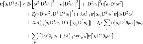 \begin{align} \textrm{tr}\big[a_{\ell}\textrm{D}^{2}\phi_{\ell}\big]&\geq 2\theta\Big[\omega^{2}\big|\textrm{D}^{3}u_{\ell}\big|^{2}+\mu\big|\textrm{D}^{2}u_{\ell}\big|^{2}\Big]+\big|\textrm{D}^{2}u_{\ell}\big|^{2}\textrm{tr}\big[a_{\ell}\textrm{D}^{2}\omega^{2}\big]\notag\\ &\quad+2\big\langle a_{\ell}\textrm{D}^{1}\omega^{2},\textrm{D}^{1}\big|\textrm{D}^{2}u_{\ell}\big|^{2}\big\rangle+\lambda A^{1}_{\varepsilon,\delta}\textrm{tr}\big[\alpha_{\ell_{0}}\textrm{D}^{2}u_{\ell}\big]\textrm{tr}\big[a_{\ell}\textrm{D}^{2}\omega\big]\notag\\ &\quad+2\lambda A^{1}_{\varepsilon,\delta}\big\langle a_{\ell}\textrm{D}^{1}\omega,\textrm{D}^{1}\textrm{tr}\big[\alpha_{\ell_{0}}\textrm{D}^{2}u_{\ell}\big]\big\rangle+2\mu\sum_{i}\textrm{tr}\big[a_{\ell}\textrm{D}^{2}\partial_{i}u_{\ell}\big]\partial_{i}u_{\ell}\notag\\ &\quad+\sum_{ji}\big[2\omega^{2}\partial_{ji}u_{\ell}+\lambda A^{1}_{\varepsilon,\delta}\omega\alpha_{\ell_{0}\,ji}\big]\textrm{tr}\big[a_{\ell}\textrm{D}^{2}\partial_{ji}u_{\ell}\big]. \end{align}
Meanwhile, differentiating twice in (3.1), we see that
 \begin{align} \textrm{tr}\big[a_{\ell}\textrm{D}^{2}\partial_{ji}u_{\ell}\big] &=\psi^{\prime\prime}_{\varepsilon,\ell}({\cdot})\bar{\eta}^{(i)}_{\ell}\bar{\eta}^{(j)}_{\ell}+\psi^{\prime}_{\varepsilon,\ell}({\cdot})\partial_{ji}\big[\big|\textrm{D}^{1}u_{\ell}\big|^{2}-g_{\ell}^{2}\big]+\sum_{\kappa\in\mathbb{I}\setminus\{\ell\}}\psi^{\prime\prime}_{\delta,\ell,\kappa}({\cdot})\bar{\eta}^{(i)}_{\ell,\kappa}\bar{\eta}^{(j)}_{\ell,\kappa}\notag\\ &\quad+\sum_{\kappa\in\mathbb{I}\setminus\{\ell\}}\psi^{\prime}_{\delta,\ell,\kappa}({\cdot})\partial_{ji}\big[u_{\ell}-u_{\kappa} \big]-\textrm{tr}\big[\partial_{j}\big[a_{\ell}\big]\textrm{D}^{2}\partial_{i}u_{\ell}\big]-\textrm{tr}\big[\big[\partial_{ji}a_{\ell}\big]\textrm{D}^{2}u_{\ell}\big]\notag\\ &\quad-\textrm{tr}\big[\big[\partial_{i}a_{\ell}\big]\textrm{D}^{2}\partial_{j}u_{\ell}\big]-\partial_{ji}\big[h_{\ell}-\big\langle b_{\ell},\textrm{D}^{1}u_{\ell}\big\rangle-c_{\ell}u_{\ell}\big], \end{align}
where
 $\bar{\eta}_{\ell}=\Big(\bar{\eta}_{\ell}^{(1)},\dots,\bar{\eta}_{\ell}^{(d)}\Big)$
and
$\bar{\eta}_{\ell}=\Big(\bar{\eta}_{\ell}^{(1)},\dots,\bar{\eta}_{\ell}^{(d)}\Big)$
and
 $\bar{\eta}_{\ell,\kappa}=\Big(\bar{\eta}_{\ell,\kappa}^{(1)},\dots,\bar{\eta}_{\ell,\kappa}^{(d)}\Big)$
with
$\bar{\eta}_{\ell,\kappa}=\Big(\bar{\eta}_{\ell,\kappa}^{(1)},\dots,\bar{\eta}_{\ell,\kappa}^{(d)}\Big)$
with
 $\bar{\eta}_{\ell}^{(i)}\,:\!=\,\partial_{i}\Big[\big|\textrm{D}^{1}u_{\ell}\big|^{2}-g_{\ell}^{2}\Big]$
and
$\bar{\eta}_{\ell}^{(i)}\,:\!=\,\partial_{i}\Big[\big|\textrm{D}^{1}u_{\ell}\big|^{2}-g_{\ell}^{2}\Big]$
and
 $\bar{\eta}_{\ell,\kappa}^{(i)}\,:\!=\,\partial_{i}[u_{\ell}-u_{\kappa} ].$
From (A.6) and (2.35)–(2.36), it follows that
$\bar{\eta}_{\ell,\kappa}^{(i)}\,:\!=\,\partial_{i}[u_{\ell}-u_{\kappa} ].$
From (A.6) and (2.35)–(2.36), it follows that
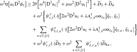 \begin{align} \omega^{2}\textrm{tr}\big[a_{\ell}\textrm{D}^{2}\phi_{\ell}\big] &\geq 2\theta\Big[\omega^{4}\big|\textrm{D}^{3}u_{\ell}\big|^{2}+\mu\omega^{2}\big|\textrm{D}^{2}u_{\ell}\big|^{2}\Big]+\widetilde{D}_{3}+\widetilde{D}_{4}\notag\\ &\quad+\omega^{2}\bigg\{\psi^{\prime\prime}_{\varepsilon,\ell}({\cdot})\big\langle\big[2\omega^{2}\textrm{D}^{2}u_{\ell}+\lambda A^{1}_{\varepsilon,\delta}\omega\alpha_{\ell_{0}}\big]\bar{\eta}_{\ell},\bar{\eta}_{\ell}\big\rangle\notag\\ &\quad+\sum_{\kappa\in\mathbb{I}\setminus\{\ell\}}\psi^{\prime\prime}_{\delta,\ell,\kappa}({\cdot})\big\langle\big[2\omega^{2}\textrm{D}^{2}u_{\ell}+\lambda A^{1}_{\varepsilon,\delta}\omega\alpha_{\ell_{0}}\big]\bar{\eta}_{\ell,\kappa},\bar{\eta}_{\ell,\kappa}\big\rangle\bigg\}\notag\\ &\quad+\omega^{2}\psi^{\prime}_{\varepsilon,\ell}({\cdot})\widetilde{D}_{5}+\omega^{2}\sum_{\kappa\in\mathbb{I}\setminus\{\ell\}}\psi^{\prime}_{\delta,\ell,\kappa}({\cdot})\widetilde{D}_{6\,\kappa}, \end{align}
where
 \begin{align*} \widetilde{D}_{3}&\,:\!=\,2\omega^{2}\big\langle a_{\ell}\textrm{D}^{1}\omega^{2},\textrm{D}^{1}\big|\textrm{D}^{2}u_{\ell}\big|^{2}\big\rangle+2\lambda A^{1}_{\varepsilon,\delta}\omega^{2}\big\langle a_{\ell}\textrm{D}^{1}\omega,\textrm{D}^{1}\textrm{tr}\big[\alpha_{\ell_{0}}\textrm{D}^{2}u_{\ell}\big]\big\rangle\notag\\ &\quad-\sum_{ij}\big[2\omega^{4}\partial_{ij}u_{\ell}+\lambda A^{1}_{\varepsilon,\delta}\omega^{3}\alpha_{\ell_{0}\,ij}\big]\big[2\textrm{tr}\big[\partial_{j}a_{\ell}\textrm{D}^{2}\partial_{i}u_{\ell}\big]-\partial_{ij}\big\langle b_{\ell},\textrm{D}^{1}u_{\ell}\big\rangle\big],\\ \widetilde{D}_{4}&\,:\!=\,\omega^{2}\big|\textrm{D}^{2}u_{\ell}\big|^{2}\textrm{tr}\big[a_{\ell}\textrm{D}^{2}\omega^{2}\big]\notag-\mu\omega^{2}\widetilde{D}_{2}u_{\ell}+\lambda A^{1}_{\varepsilon,\delta}\omega^{2}\textrm{tr}\big[\alpha_{\ell_{0}}\textrm{D}^{2}u_{\ell}\big]\textrm{tr}\big[a_{\ell}\textrm{D}^{2}\omega\big]\notag\\ &\quad-\sum_{ji}\big[2\omega^{4}\partial_{ji}u_{\ell}+\lambda A^{1}_{\varepsilon,\delta}\omega^{3}\alpha_{\ell_{0}\,ji}\big]\left\{\textrm{tr}\big[\big[\partial_{ji}a_{\ell}\big]\textrm{D}^{2}u_{\ell}\big]+\partial_{ji}\big[h_{\ell}-c_{\ell}u_{\ell}\big]\right\},\\ \widetilde{D}_{5}&\,:\!=\, 2\mu\big\langle \textrm{D}^{1}u_{\ell},\bar{\eta}_{\ell}\big\rangle+\textrm{tr}\big[\big[2\omega^{2}\textrm{D}^{2}u_{\ell}+\lambda A^{1}_{\varepsilon,\delta}\omega\alpha_{\ell_{0}}\big]\textrm{D}^{2}\big[\big|\textrm{D}^{1}u_{\ell}\big|^{2}-g_{\ell}^{2}\big]\big],\\ \widetilde{D}_{6\,\kappa}&\,:\!=\, 2\mu\big\langle \textrm{D}^{1}u_{\ell},\bar{\eta}_{\ell,\kappa}\big\rangle+\textrm{tr}\big[\big[2\omega^{2}\textrm{D}^{2}u_{\ell}+\lambda A^{1}_{\varepsilon,\delta}\omega\alpha_{\ell_{0}}\big]\textrm{D}^{2}\big[u_{\ell}-u_{\kappa} \big]\big]. \end{align*}
Recall that
 $\widetilde{D}_{2}u_{\ell}$
is given in (A.7). To obtain the next inequalities, we shall recurrently use (H3), (H4), Remark 3.1, (3.2), (3.3), and
$\widetilde{D}_{2}u_{\ell}$
is given in (A.7). To obtain the next inequalities, we shall recurrently use (H3), (H4), Remark 3.1, (3.2), (3.3), and
 $\lambda,\mu\geq1$
. Then,
$\lambda,\mu\geq1$
. Then,
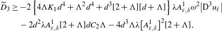 \begin{align} \widetilde{D}_{3} &\geq-2\left\{4\Lambda K_{1}d^{4}+\Lambda^{2} d^{4}+d^{3}[2+\Lambda][d+\Lambda]\right\}\lambda A^{1}_{\varepsilon,\delta}\omega^{2}\big|\textrm{D}^{3}u_{\ell}\big|\notag\\ &\quad-2d^{2}\lambda A^{1}_{\varepsilon,\delta}[2+\Lambda]dC_{2}\Lambda-4d^{3}\Lambda\lambda\big[A^{1}_{\varepsilon,\delta}\big]^{2}[2+\Lambda], \end{align}
and by (2.11),
 \begin{align} \widetilde{D}_{4} &\geq-\big\{2\Lambda d^{2}K_{1}+ d^{4}\Lambda^{2}K_{1}+d^{2}\Lambda\big[2+\Lambda\big]\big[d^{2}+1\big]\big\}\lambda\big[A^{1}_{\varepsilon,\delta}\big]^{2}\notag\\ &\quad-\big\{2\mu\big[2C_{2}\Lambda d^{3}+2d^{1/2}\Lambda C_{2}\big]+d^{2}\lambda\Lambda\big[2+\Lambda\big]\big[2C_{2}+C_{1}\big]\big\}A^{1}_{\varepsilon,\delta}\notag\\ &\quad-2\mu\big\{2C_{2}\Lambda d^{2}+2C_{1}C_{2}d^{1/2}\Lambda-2C_{2}\Lambda d^{1/2}\big\}. \end{align}
On the other hand, since
 $\lambda\geq\frac{2}{\theta}$
and using (2.11), we have that
$\lambda\geq\frac{2}{\theta}$
and using (2.11), we have that
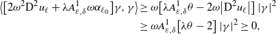 \begin{align} \big\langle\big[2\omega^{2}\textrm{D}^{2}u_{\ell}+\lambda A^{1}_{\varepsilon,\delta}\omega\alpha_{\ell_{0}}\big]\gamma,\gamma\big\rangle&\geq\omega\big[\lambda A^{1}_{\varepsilon,\delta}\theta-2\omega\big|\textrm{D}^{2}u_{\ell}\big|\big]\,|\gamma|^{2}\notag\\ & \geq\omega A^{1}_{\varepsilon,\delta}\big[\lambda\theta-2\big]\,|\gamma|^{2}\geq0, \end{align}
for
 $\gamma\in\mathbb{R}^{d}$
. From here and since
$\gamma\in\mathbb{R}^{d}$
. From here and since
 $\psi^{\prime\prime}_{\varepsilon,\ell}({\cdot})\geq0$
and
$\psi^{\prime\prime}_{\varepsilon,\ell}({\cdot})\geq0$
and
 $\psi^{\prime\prime}_{\delta,\ell,\kappa}({\cdot})\geq0$
, it follows that
$\psi^{\prime\prime}_{\delta,\ell,\kappa}({\cdot})\geq0$
, it follows that
 \begin{align} \psi^{\prime\prime}_{\varepsilon,\ell}({\cdot})\big\langle\big[2\omega^{2}\textrm{D}^{2}u_{\ell} & +\lambda A^{1}_{\varepsilon,\delta}\omega\alpha_{\ell_{0}}\big]\bar{\eta}_{\ell},\bar{\eta}_{\ell}\big\rangle \nonumber\\& +\sum_{\kappa\in\mathbb{I}\setminus\{\ell\}}\psi^{\prime\prime}_{\delta,\ell,\kappa}({\cdot})\big\langle\big[2\omega^{2}\textrm{D}^{2}u_{\ell}+\lambda A^{1}_{\varepsilon,\delta}\omega\alpha_{\ell_{0}}\big]\bar{\eta}_{\ell,\kappa},\bar{\eta}_{\ell,\kappa}\big\rangle\geq0.\end{align}
It is easy to verify that
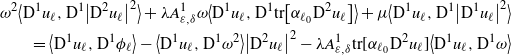 \begin{align} \omega^{2}\big\langle \textrm{D}^{1}u_{\ell},\textrm{D}^{1}\big|\textrm{D}^{2}u_{\ell}\big|^{2}\big\rangle+\lambda A^{1}_{\varepsilon,\delta}\omega\big\langle \textrm{D}^{1}u_{\ell},\textrm{D}^{1}\textrm{tr}\big[\alpha_{\ell_{0}}\textrm{D}^{2}u_{\ell}\big]\big\rangle+\mu\big\langle \textrm{D}^{1}u_{\ell},\textrm{D}^{1}\big|\textrm{D}^{1}u_{\ell}\big|^{2}\big\rangle\nonumber\\ =\big\langle \textrm{D}^{1}u_{\ell},\textrm{D}^{1}\phi_{\ell}\big\rangle-\big\langle \textrm{D}^{1}u_{\ell},\textrm{D}^{1}\omega^{2}\big\rangle\big|\textrm{D}^{2}u_{\ell}\big|^{2}-\lambda A^{1}_{\varepsilon,\delta}\textrm{tr}[\alpha_{\ell_{0}}\textrm{D}^{2}u_{\ell}]\big\langle \textrm{D}^{1}u_{\ell},\textrm{D}^{1}\omega\big\rangle\end{align}
since
 \begin{align*} \partial_{i}\phi_{\ell}&=\big|\textrm{D}^{2}u_{\ell}\big|^{2}\partial_{i}\omega^{2}+\omega^{2}\partial_{i}\big|\textrm{D}^{2}u_{\ell}\big|^{2}\\ &\quad+\lambda A^{1}_{\varepsilon,\delta}\textrm{tr}\big[\alpha_{\ell_{0}}\textrm{D}^{2}u_{\ell}\big]\partial_{i}\omega+\lambda A^{1}_{\varepsilon,\delta}\omega \textrm{tr}\big[\alpha_{\ell_{0}}\textrm{D}^{2}\partial_{i}u_{\ell}\big]+\mu\partial_{i}\big|\textrm{D}^{1}u_{\ell}\big|^{2}\quad\text{on}\ B_{\beta r}. \end{align*}
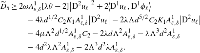 \begin{align} \widetilde{D}_{5} &\geq2\omega A^{1}_{\varepsilon,\delta}[\lambda\theta-2]\big|\textrm{D}^{2}u_{\ell}\big|^{2}+2\big\langle \textrm{D}^{1}u_{\ell},\textrm{D}^{1}\phi_{\ell}\big\rangle\notag\\ &\qquad-4\lambda d^{1/2}C_{2}K_{1}A^{1}_{\varepsilon,\delta}\big|\textrm{D}^{2}u_{\ell}\big|-2\lambda\Lambda d^{5/2}C_{2}K_{1}A^{1}_{\varepsilon,\delta}\big|\textrm{D}^{2}u_{\ell}\big|\notag\\ &\qquad-4\mu \Lambda^{2}d^{1/2}A^{1}_{\varepsilon,\delta}C_{2}-2\lambda d\Lambda^{2}A^{1}_{\varepsilon,\delta}-\lambda\Lambda^{3}d^{2}A^{1}_{\varepsilon,\delta}\notag\\ &\qquad-4d^{2}\lambda\Lambda^{2}A^{1}_{\varepsilon,\delta}-2\Lambda^{3}d^{2}\lambda A^{1}_{\varepsilon,\delta}. \end{align}
Using the properties
 $|A|^{2}-2\textrm{tr}[AB]+|B|^{2}=\sum_{ij}\big(A_{ij}-B_{ij}\big)^{2}\geq0$
and
$|A|^{2}-2\textrm{tr}[AB]+|B|^{2}=\sum_{ij}\big(A_{ij}-B_{ij}\big)^{2}\geq0$
and
 $|y_{1}|^{2}-2\langle y_{1},y_{2}\rangle+|y|^{2}=\sum_{i}(y_{1,i}-y_{2,i})^{2}\geq0$
, where
$|y_{1}|^{2}-2\langle y_{1},y_{2}\rangle+|y|^{2}=\sum_{i}(y_{1,i}-y_{2,i})^{2}\geq0$
, where
 $A=(A_{ij})_{d\times d}$
,
$A=(A_{ij})_{d\times d}$
,
 $B=(B_{ij})_{d\times d}$
, and
$B=(B_{ij})_{d\times d}$
, and
 $y_{1}=(y_{1,2},\dots,y_{1,d}),y_{2}=(y_{2,1},\dots,y_{2,d})$
belong
$y_{1}=(y_{1,2},\dots,y_{1,d}),y_{2}=(y_{2,1},\dots,y_{2,d})$
belong
 $\mathcal{S}(d)$
and
$\mathcal{S}(d)$
and
 $\mathbb{R}^{d}$
, respectively, and by definition of
$\mathbb{R}^{d}$
, respectively, and by definition of
 $\phi_{\ell}$
, it is easy to corroborate the following identity:
$\phi_{\ell}$
, it is easy to corroborate the following identity:
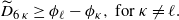 \begin{equation} \widetilde{D}_{6\,\kappa}\geq \phi_{\ell}-\phi_{\kappa} ,\ \text{for}\ \kappa\neq\ell. \end{equation}
Applying (A.41)–(A.44) in (A.37) and considering that all constants that appear in those inequalities (i.e. (A.41)–(A.44)) are bounded by a universal constant
 $C_{7}=C_{7}(d,\Lambda,\alpha^{\prime},K_{1})$
, we obtain the desired result in the lemma above. With this remark, the proof is concluded.
$C_{7}=C_{7}(d,\Lambda,\alpha^{\prime},K_{1})$
, we obtain the desired result in the lemma above. With this remark, the proof is concluded.
Acknowledgements
The authors would like to thank the anonymous reviewers for their comments and suggestions, which improved the quality of this paper.
Funding information
The authors were supported by the Russian Academic Excellence Project 5-100.
Competing interests
There were no competing interests to declare which arose during the preparation or publication process for this article.


