History

Early astronomers grappled with differences in measurement between raters and over time. In 1632, Galileo noted that errors in observation were usually symmetrically distributed around a true value and had a central tendency such that large errors were less common than small ones Reference Stahl(1). Later astronomers typically averaged discrepant observations, until, in 1809, Carl Gauss derived the formula for what we now recognize as the normal distribution. He called this the ‘Curve of Errors' and demonstrated its application in the prediction of planetary orbits. The curve was also formulated at the same time by the mathematician Laplace, and hence the curve was often referred to as a ‘Gaussian’ or ‘Laplacian’ distribution.

The application of this ‘Curve of Errors' became widespread in areas ranging from natural sciences to probability theory and gambling. The naturalist and philosopher Francis Galton described it as the ‘Normal Curve of Frequency’ and famously said of the rules underlying it: ‘The law would have been personified by the Greeks and deified, if they had known of it. It reigns with serenity and in complete self-effacement, amidst the wildest confusion. The huger the mob, and the greater the apparent anarchy, the more perfect is its sway. It is the supreme law of Unreason.’ Reference Galton(2).

The popularization of the term ‘normal distribution’ is attributed to the statistician Karl Pearson, who later expressed concern that the widespread use of the term had come to imply that the many other possible distributions were somehow abnormal Reference Stahl(1).

Properties of the normal distribution

The mathematical properties of the normal distribution are familiar. A normal curve is a symmetrical distribution where the frequency of occurrence reduces as the distance from the mean increases, approaching zero asymptotically at both extremes. The prototypic curve is expressed as having a mean of zero and a standard deviation of one. Sixty-eight percent (68%) of values fall within one standard deviation of the mean, and ninety-five percent (95%) fall within two standard deviations of the mean. There is an infinite variety of possible normal curves, defined by differences in the two key parameters (mean and standard deviation); however, these differ only in scale and not in fundamental shape.

Which properties of an underlying process are likely to result in values forming a normal distribution? Such phenomena are likely to have (a) a natural or central limit, (b) random variation around that limit and (c) some form of ‘attractor’ such that values are likely to cluster around the central limit, with large variations from that limit less likely than small ones.

It is easy to see how the early astronomical ‘Curve of Errors' had these properties: the true value being observed effectively forms the mean and attractor. However, for normally distributed phenomena within populations (e.g. height, chest circumference and IQ) the term ‘error’ is misleading. Here, the population mean does not represent an underlying ‘true’ value. Rather than errors of observation, random variation around the population mean occurs as a result of interactions of genetic, developmental, cultural and/or other factors.

Under some circumstances normal distributions also arise from phenomena which are not normally distributed. Laplace's Central Limit Theorem proved that the means of a series of random samples from a distribution will be normally distributed, regardless of the shape of that underlying distribution: the distribution of sample means becomes more normal as sample size increases Reference Tabachnick and Fidell(3). Figure 1 shows this effect. Data are length of stay for 25 896 separations from mental health units, trimmed to remove day-only stays and stays above the 95th percentile. The distribution is highly skewed. One hundred random samples were drawn from this data. As sample size increases the distribution of sample means becomes increasingly normal, even though individual samples are themselves not normally distributed.

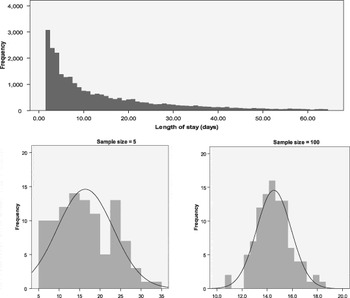
Fig. 1 Central limit theorem. Distribution of means of 100 random samples from a skewed distribution of Length of Stay. As sample size increases, sample means become normally distributed.

Departures from normality: skewness and kurtosis

One defining characteristic of the normal distribution is its symmetry. Skewness refers to the symmetry of a distribution. A skewed distribution is an asymmetrical one and ‘a skewed variable is a variable whose mean is not in the centre of the distribution’Reference Tabachnick and Fidell(3).

The degree of skewness of a distribution can be described numerically. A normal distribution has a skewness of zero. The polarity of skewness is defined by the tail of the skewed distribution: a positively or right skewed distribution has more values to the left and fewer values (the tail) to the right (Fig. 2).

Fig. 2 Skewness.

For natural phenomena, skewed distributions may arise where a natural limit prevents symmetry by imposing a fixed maximum or minimum value on a population, or where variations arise through systematic and non-linear processes rather than random variations. Many phenomena in psychiatry may have skewed distributions, including rates of suicide attempts Reference Bateman and Fonagy(4), substance abuse rates Reference Delucchi and Bostrom(5) and duration of untreated psychosis (DUP) (Reference Compton, Ramsay and Shim6–Reference Large, Nielssen, Slade and Harris8).

Measures of health care use such as length of hospital stay Reference Kunik, Cully, Snow, Souchek, Sullivan and Ashton(9,Reference Durbin, Lin, Layne and Teed10), health care costs Reference Buntin and Zaslavsky(11,Reference Kilian, Matschinger, Loeffler, Roick and Angermeyer12), and number of hospitalizations or out-patient visits Reference Fikretoglu, Elhai, Liu, Richardson and Pedlar(13) typically have skewed distributions. Such distributions often have large numbers of individuals with zero values, are intrinsically asymmetric (it is impossible to have negative service use) and include a small number of outliers with very large utilization and cost.

The second defining characteristic of the normal distribution is the extent of central clustering of values around the mean, also called the kurtosis of the distribution. Expressed numerically, the normal distribution has a kurtosis of three: the kurtosis of a sample distribution is typically expressed as a difference from three, so that a sample with normal distribution has an excess kurtosis of zero. Higher (positive) values of kurtosis describe a ‘tall’ distribution with values more closely clustered around the mean and fewer values in the tails of the distribution. Lower (negative) values of kurtosis describe a broad, shallow distribution with fewer values near the mean and a higher proportion of values at a distance from the mean (Fig. 3).

Fig. 3 Kurtosis.

The normal distribution and parametric statistics

Many common statistical techniques (e.g. Student's t-test, Analysis of Variance, Pearson's correlation and Linear Regression) are of a class known as parametric statistics. They are based on assumptions about the distribution of the underlying data, and are appropriately used for normally distributed data. Recent editions of this journal demonstrate the continuing utility of these techniques in psychiatric research for data ranging from psychometric questionnaires and scales (Reference Mortensen, Rasmussen and Håberg14–Reference Walter, Byrne and Griffiths16) to MRI and EEG parameters Reference Calhoun, Wu, Kiehl, Eichele and Pearlson(17,Reference Sui, Wu and King18).

Many studies using parametric techniques do not state explicitly whether assumptions regarding the distribution of the data have been tested. The reader must assume that a reviewer has been satisfied that such testing has been done, or consider whether the data being described would typically fit a normal distribution.

The violation of the assumption of normality in parametric statistics may result in incorrect inference. However, some parametric tests (e.g. Student's t-test and Linear Regression) are robust to violations of the assumption of normality where sample size is large. This is due to the impact of the Central Limit Theorem: with larger sample size, sample means tend to be normally distributed even when drawn from an underlying non-normal distribution. Lumley et al. Reference Lumley, Diehr, Emerson and Chen(19) review this issue and argue that most public health datasets are sufficiently large that t-tests may be applied even for highly skewed data such as health care costs. The arguments are supported by simulation data Reference Shuster(20).

Testing for normality

Because of these impacts, the distribution of data should be tested before parametric techniques are applied. There are several possible methods for such testing.

Visual comparison using frequency histograms or probability plots (PPs) provides a simple screening method for identifying highly non-normal data; however, more formal methods are required.

The numerical values of skew and kurtosis for a sample may be examined with several rules of thumb. Skew and kurtosis should ideally be close to zero. Absolute skewness values between 0.5 and 1 are typically seen as indicating moderately skewed data, and greater than 1 as indicating highly skewed data. For kurtosis, an often cited rule Reference Tabachnick and Fidell(3) is that kurtosis is excessively high or low if the measured kurtosis is greater than plus or minus twice the ‘standard error of kurtosis' (SEK), which is estimated as the square root of twenty four divided by the sample size (i.e. SEK = √(24/N)).

Several statistical techniques examine both skewness and kurtosis to provide an overall probability that a sample of data has been drawn from a normal distribution. The Kolmogorov–Smirnov test is a non-parametric test that may be used to compare any two distributions, but is often used to compare a sample distribution with the idealized normal distribution. It is based on the construction of a cumulative fraction plot, which plots sorted data points on the x-axis against the cumulative percentage of the sample falling below that x value. This creates a cumulative distribution curve, which can be compared against the cumulative curve of the normal distribution. The significance of difference between the two datasets is calculated using the ‘D’ statistic, representing the maximum vertical distance between the two cumulative distribution curves.

The Kolmogorov–Smirnov test compares two samples. Where a sample distribution is being compared with a population distribution (e.g. the normal distribution) a modified version of the test, the Lilliefors modification, is used, and the test may also be referred to as the KS–Lilliefors test.

The Shapiro–Wilks test is based on the normal PPs (P–P plot): for a normally distributed variable, this PP plot forms a straight line. The Shapiro–Wilks test calculates the correlation coefficient of observed data with this expected line, expressing this as ‘W’. Low correlation indicates departure from normality. This test is often recommended for smaller sample sizes (less than 50) but may not perform well where there are large numbers of tied values in the sample.

Table 1 provides an example of these tests, applied to the distribution of sample means used to demonstrate the Central Limit Theorem in Fig. 1. One hundred random samples were drawn from a large skewed dataset (hospital length of stay) for each of a range of sample sizes from five to one hundred. As sample size increases, sample means converge on the population mean and skewness and kurtosis reduce. At larger sample sizes, both Kolmogorov–Smirnov and Shapiro–Wilks tests suggest that the sample distributions do not differ significantly from a normal distribution (p > 0.05). This example tests the distribution of sample means; however, these tests would more usually be applied to compare two samples or a single sample with a normal population distribution: in these situations larger sample sizes would usually be required.

Table 1 Normality testing in central limit theorem. Data as per Fig. 1: 100 random samples from a skewed distribution (length of stay). As sample size increases, the sample means become normally distributed and approach the population mean. At sample sizes of 20 and above the distribution of sample means did not differ significantly from a normal distribution

* p < 0.05 indicates significant departure from a normal distribution.

Other widely used tests of normality include the Anderson–Darling and chi-squared goodness of fit tests.

It should also be noted that for more complex parametric statistics, such as multiple regressions, the assumptions of normality apply to the residuals of the regression model rather than to the raw data, and it is therefore these residuals that should be tested as part of the diagnostic phase of the regression.

Transformation

Where data is not normally distributed there are several possible approaches. For some applications it may be possible to use the median as an alternative measure of central tendency. However, while this may be informative for descriptive statistics (e.g. Compton Reference Compton, Ramsay and Shim(6) reports median DUP), the median is rarely used in inferential statistics. For highly skewed distributions, e.g. distributions with many zero values, the median may itself be zero, providing limited descriptive value.

Therefore, transformation is often the first strategy attempted in dealing with non-normal data. Transformation involves application of a mathematical function to the data in order to change its distribution. The aim of transformation is to return a variable to a sufficiently normal distribution so that parametric statistics may then be applied.

The type of transformation applied depends on both the type and extent of departure from normality. Skewness may be corrected using square root transformation if mild, log transformation if moderate and inverse transformation if severe Reference Tabachnick and Fidell(3). A constant may be introduced to the transformation to remove zero values or change the direction of negative skewness; however, transformation approaches may still fail to normalize the distribution where there are large numbers of zero values Reference Delucchi and Bostrom(5).

Kurtosis is typically corrected using power transformations, e.g. square root or cube root transformations for variables with excessive positive kurtosis, or the inverse of these functions for variables with excessive negative kurtosis.

Several recent publications provide examples of these transformation approaches in psychiatry. Hanrahan et al. Reference Hanrahan, Kumar and Aiken(21) examined hospital incident data to identify organization factors that predicted adverse incidents in general hospital psychiatry units. Staffing data (nurse to patient ratios) had a significantly skewed distribution. These were therefore log transformed to allow application of a linear regression model. Nurse to patient ratios were found to have a significant association with incidents of staff injury, but not with other incident types such as falls, medication errors or complaints.

Thomas et al. Reference Thomas, Waxmonsky, Gabow, Flanders-Mcginnis, Socherman and Rost(22) examined the impact of psychiatric disorders on overall health care expenditure within an American health care organisation. Because cost per person was highly skewed, this data was log transformed: differences between groups in this log-transformed data were then examined using Analysis of Covariance (ANCOVA) with covariates including age, gender and health plan variables.

Venneman et al. Reference Venneman, Leuchter and Bartzokis(23) examined for neurophysiological (EEG) predictors of dropout during cocaine treatment. The distribution of EEG power values at each electrode demonstrated both skewness and kurtosis: the values were square root transformed before analysis.

Buntin and Zaslavsky Reference Buntin and Zaslavsky(11) pointed out that there is no single ideal method for transformation: different methods may be appropriate depending on the research question being examined. While transformation of variables in this way has advantages in that it allows the use of familiar and robust parametric techniques, it also has disadvantages. Transformed data may be difficult to interpret. For example, log transformation of a service variable (such as length of stay) or clinical variable (such as a score on a depression rating scale) may be statistically appropriate, but the meaning of the transformed variable may no longer be easily interpreted (what would it mean to show that an intervention resulted on average in a one unit change in the log of a persons's depression rating?). This is sometimes addressed by re-transformation of results back into the original scale. However, this may result in significant errors (‘smearing’) and imprecision.

Non-parametric approaches

Where transformation has not been possible or is inappropriate, a wide variety of non-parametric tests may be employed. These tests make fewer assumptions about the distributions of the underlying data than parametric tests, and are sometimes referred to as ‘distribution free’.

One common approach is to collapse or convert a skewed continuous measure into a categorical measure with two more levels. This allows the use of common non-parametric techniques such as chi-square analysis or logistic regression. For example Kunik et al. Reference Kunik, Cully, Snow, Souchek, Sullivan and Ashton(9) examined whether treatable co-morbidities (e.g. pain, depression) were associated with increased service use for persons with dementia. Hospitalization data was skewed, and there were large numbers of persons with no bed days. Therefore data was collapsed into two groups, those with and without hospital bed days, which were then compared using binary logistic regression. However, there are many disadvantages to categorizing a continuous variable Reference Senn and Julious(24), including loss of information and substantial loss of statistical power. Altman and Royston Reference Altman and Royston(25) point out that the common technique of dichotomizing a variable at the median produces a loss of statistical power equivalent to discarding a third of the data, and splits at points other than the median may produce even larger losses of power.

For many study designs it is necessary to use a non-parametric approach which allows the variable of interest to continue to be treated as a continuous variable. This paper cannot aim to review all such possible methods; however, the following recent publications give some examples of these approaches.

Bateman and Fonagy Reference Bateman and Fonagy(4) examined whether mentalisation based psychotherapy reduced suicide attempts in persons with Borderline Personality Disorder. They compared the number of suicide attempts over a five-year period in 22 experimental subjects and 19 treatment as usual controls. The distribution of suicide attempts was highly skewed. Therefore differences between groups were examined using the Mann–Whitney U test (also known as Wilcoxon's rank sum test). This widely used test uses sorted rank order rather than absolute value as its basis for comparison between groups. (An alternative approach to this study may have been to have treated the number of suicide attempts as count data potentially following a Poisson or Binomial distribution and then used an appropriate test for comparing the means of two samples with these distributions, such as the C-test or Fishers Exact test.)

The Mann–Whitney U test was also used by Ho et al. Reference Ho, Alicata and Ward(7), who examined untreated psychosis (DUP) as an independent variable, assessing its role in predicting neuro-cognitive function in young people with psychosis. Because of the skewed distribution of DUP, the group was divided at the median into two categories (short and long DUP). Spearman's rank order correlation coefficients were also used to examine the relationship between DUP and performance on specific cognitive test domains.

Compton et al. Reference Compton, Ramsay and Shim(6) used DUP as a dependent variable, examining health service, social and demographic factors which predicted longer DUP. Because of the skewed distribution of DUP, the log-rank test was employed. This test, also called the Mantel–Cox test, is used for survival analysis with right-censored data (e.g. time to admission/relapse).

Fikretoglu et al. Reference Fikretoglu, Elhai, Liu, Richardson and Pedlar(13) used data from an epidemiological survey of Canadian military veterans, examining whether mental health diagnoses, demographic factors or military service factors predicted the use of mental health or general health services. Service use variables (e.g. mental health provider visits or doctor visits per person) were highly skewed and included significant numbers of zero values. Standard log transformation could not normalize the data. Therefore, Zero-Inflated Negative Binomial Regression was used to calculate odds ratios for likelihood of service use in the last 12 months.

Analysis of skewed health care cost data often employs “two part” models which combine several of the features described above. Where there are many zero values, analyses may first collapse data into zero and non-zero groups, comparing these categorically with a technique such as logistic regression. Then, as a second stage of analysis, the non-zero values are examined as continuous variables using an appropriate parametric or non-parametric regression technique. Detailed review and simulation of these models can be found in Buntin and Zaslavsky Reference Buntin and Zaslavsky(11) and Delucchi and Bostrom Reference Delucchi and Bostrom(5).

The complexity of the issues in choosing an appropriate analysis method for skewed data is shown by Kilian et al. Reference Kilian, Matschinger, Loeffler, Roick and Angermeyer(12). They compared three regression approaches to predict the annual cost of health care for 254 persons with Schizophrenia. These costs had a skewed distribution. Three methods were compared: linear (ordinary least squares, or OLS) regression on raw data, linear regression on log-transformed data, and a more complex generalized linear model (GLM) regression. They compared the performance of these three approaches on a range of parameters. Differences between models were subtle and did not always favour the more complex models. Surprisingly, they found that the OLS regression model on untransformed data performed best overall; however, they cautioned that their sample size was small and that this may not apply to all situations.

Conclusions

From suicide attempts and DUP to health care service utilization and cost, many important phenomena in psychiatry have skewed or otherwise non-normal distributions.

In their recent review of techniques for analysis of skewed data in psychiatry, Delucchi and Bolstrom Reference Delucchi and Bostrom(5) concluded that ‘The purpose of considering methods alternative to the standard classic parametric tests such as the t test and the least-squares repeated-measures ANOVA is not to buy a better result–that will most often not be the case–but rather to buy legitimacy as a safeguard against a type I error.’

A psychiatrist should bear in mind the power and elegance of the normal distribution and the risks of incorrect inference if parametric statistics are applied to non-normal data.